A Real-Time Early Warning Seismic Event Detection Algorithm Using Smart Geo-Spatial Bi-Axial Inclinometer Nodes for Industry 4.0 Applications

 ,
,
Abstract
1. Introduction
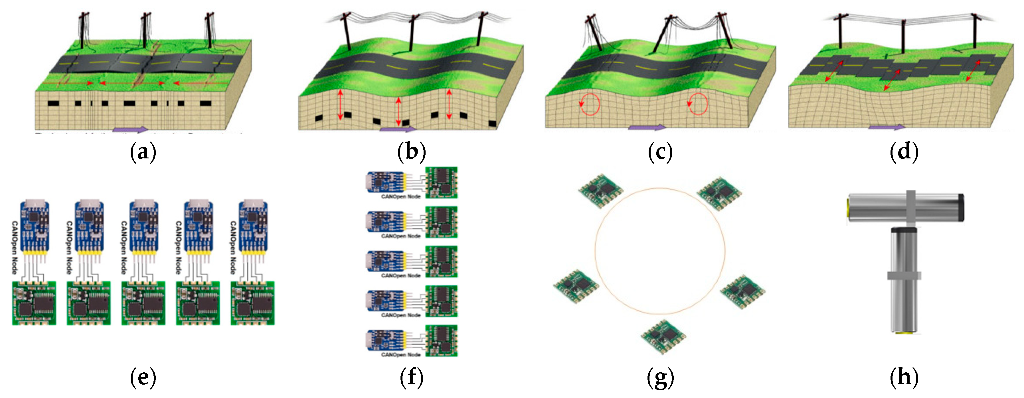
- (a)
- A geo-seismic constraint sensing node with ADC comprised of 2+ times higher sampling frequency for seismic signals as per the Nyquist criterion and a resolution of ±0.0000X.
- (b)
- Normalization of a single geo-seismic sensing node (GSSN) or ISCS magnitude offsets induced by placement errors.
- (c)
- Normalization of clustered GSSNs or ISCS magnitudes complex orientation errors.
- (d)
- Heterogeneous surface orientation errors were reflected in entire measurements and geo-seismic data processing.
- (e)
- Gaussian or pseudo-random noise issues in the form of high frequencies and nano- or micro-seismic angular displacement anomalies.
- (f)
- Sequential detection of incremental displacement amplitudes to reduce post-computation costs and predict the upcoming threats [11] as primary, secondary, and tertiary alarms.
- (g)
- Adaptive amplitude real-time thresholds mapping to reduce incremental filtering costs.
- (h)
- Real-time estimation of pre-triggering and post-triggering parameters for recording or event capturing algorithms based on amplitudes, number of samples, and obliged frequencies.
- (i)
- Runtime or real-time similarity in amplitudes and frequencies with existing time series of earthquakes that happened in the past in parallel and compare triggering time intervals as discrete occurrences instead.
- (j)
- The geometrical exploration of seismic wave kinematics (frequency and amplitudes of two-dimensional angular displacements) for maximum details required for the geo-seismic realization using algorithmic calibration.
- (k)
- Methodological, adaptive, and event-driven sensor calibration and measurement optimization capability nodes are enablement towards Industry 4.0 applications.
- (l)
- Real-time remote calibration of ADC parameters to optimize low-cost geo-seismic detection using error-compensated, de facto, de jure industry-standard communication buses. This capability constitutes a steppingstone towards Industry 4.0-based condition monitoring benchmarks.
- (m)
- Sustainable distant and chronological optimization of real-time seismic event detection.
- (n)
- Adaptive real-time scaling of sensors to zoom+/zoom− in case of micro/macro magnitudes for iterative optimization.
- (o)
- The real-time sensor calibration and recording triggering feature for unit sensor nodes as well as sensor clusters is the Industry 4.0 application benchmark for SWEDA.
- Real-time seismic wave event detection algorithm (SWEDA) for cyber-physical systems.
- Smart geospatial bi-axial inclinometer nodes (SGBINs) application design for SWEDA.
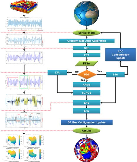
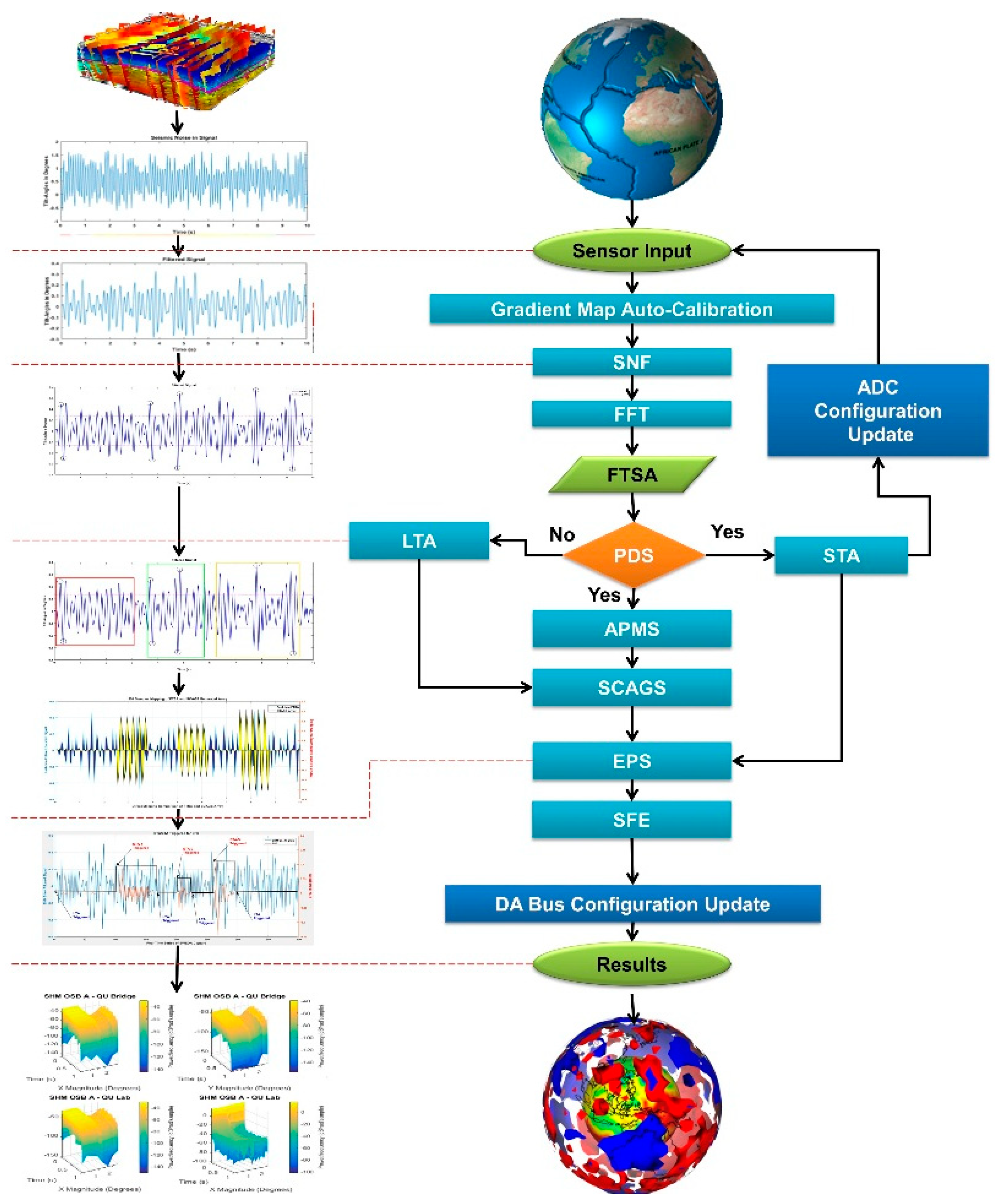
2. Methodology Architecture
- Gradient map auto-calibration (GMAC)
- Micro-seism or seismic noise filtration (SNF)
- Peak detection sequence (PDS)
- Autoregressive pattern mapping sequence (APMS)
- Scaling coefficients array generation sequence (SCAGS)
- STA/LTA arrays windows sequence (SLAWS)
- Earthquake probabilistic sequence (EPS)
- Seismic features extraction (SFE)
- ADC scaling/range and communication bus configuration
- MATLAB for Desktop PC Workstation.
- MATLAB Coder for Raspberry Pi.
- Python 2.7 for Single Board Computer (Raspberry Pi).
2.1. Gradient Mapping and Auto-Calibration (GMAC)
2.2. Seismic Noise Filtration (SNF)
2.3. Peak Detection Sequence (PDS)
2.4. Autoregressive Pattern Mapping Sequence (APMS)
2.5. Scaling Coefficients Array Generation Sequence (SCAGS)
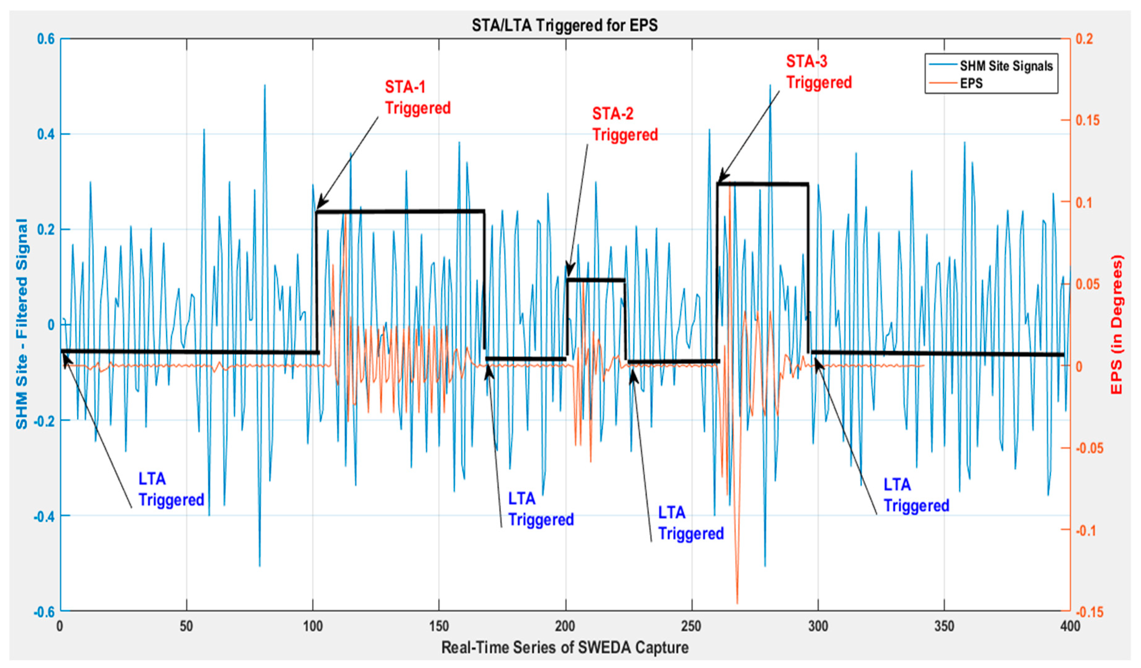
2.6. STA/LTA Arrays Windows Sequence (SLAWS)
- Wd—Waveform data (‘shm_thingspeak.csv’)
- Fs—Sampling frequency (as per Nyquist criterion, i.e., 2F = 2 (1 Hz), 2 (1.5 Hz), … 2 (24 Hz))
- Lts—Length of time series (80,000 samples)
- Tv—Time vector of the waveform (10,000 samples)
- ABSts—Absolute value of time series (40,000)
- WSTA = EDP1*Fs − STA window size (Dynamic)
- WLTA = EDP2*Fs − LTA window size (Dynamic)
- WLLTA = WLLTA − current length of growing LTA window (sizes of the time axis of respective wave)
- TRON-STA+LTA = EDP3 − trigger on when STA_to_LTA exceeds this threshold
- TRON-STA-LTA = EDP4 − trigger off when STA_to_LTA drops below the threshold
2.7. Earthquake Probabilistic Sequence (EPS)
2.8. Seismic Feature Extraction (SFE)
2.9. Event-Triggered ADC Scaling/Range and Communication Bus Configuration
3. Smart Geo-Spatial Inclinometer Nodes Application Design
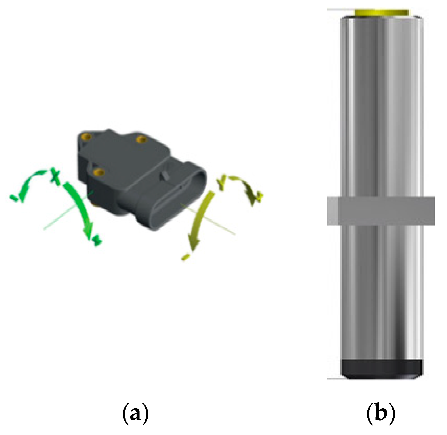
- Flat SGSINs with two accelerometers used as inclinometer sensors (F-SGSINs)
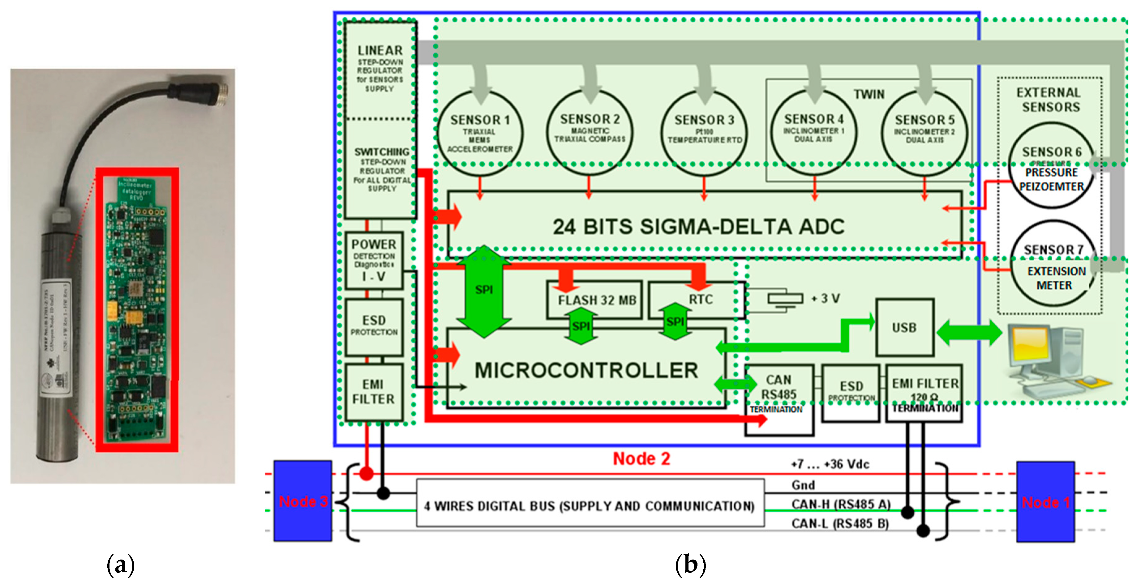
- Cylindrical SGSINs with 2 + N sensor support (C-SGSINs)
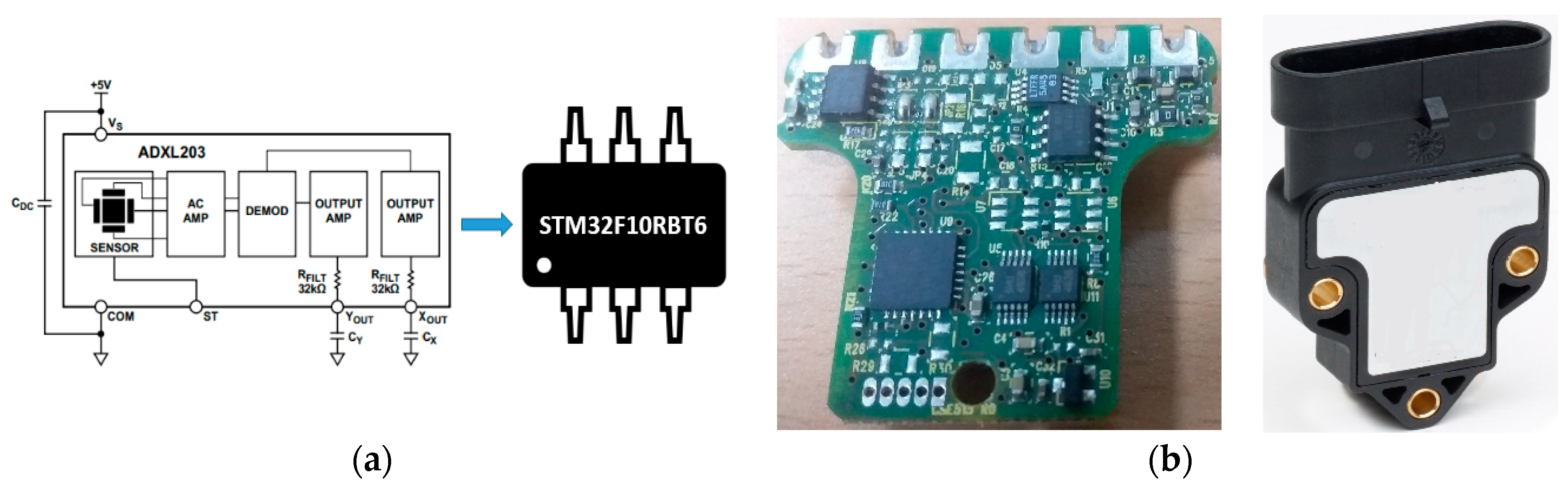
3.1. Flat SGSINs
3.2. Cylindrical SGBINs
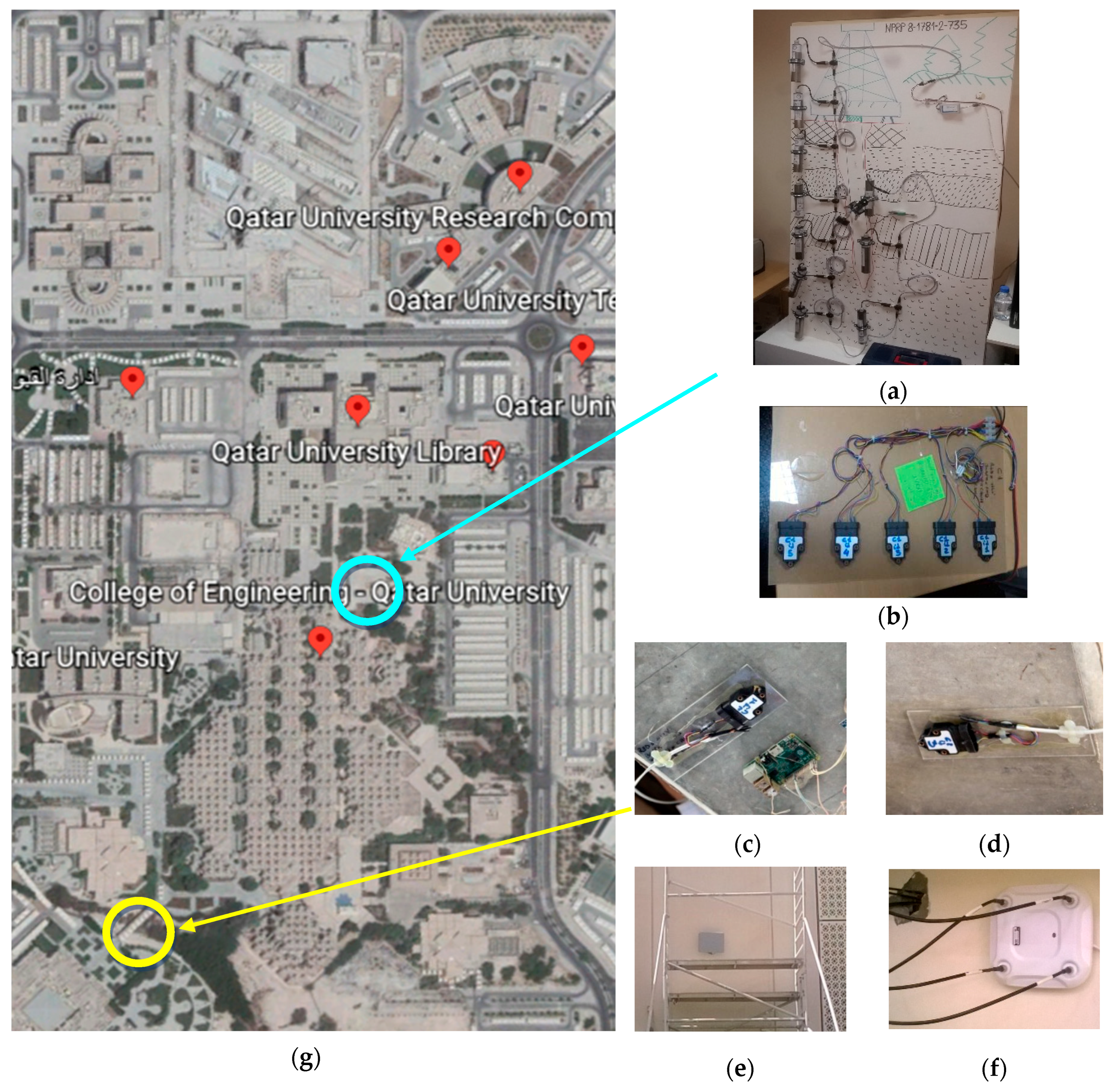
4. Case Study: Experiment Designed and Implemented at Qatar University
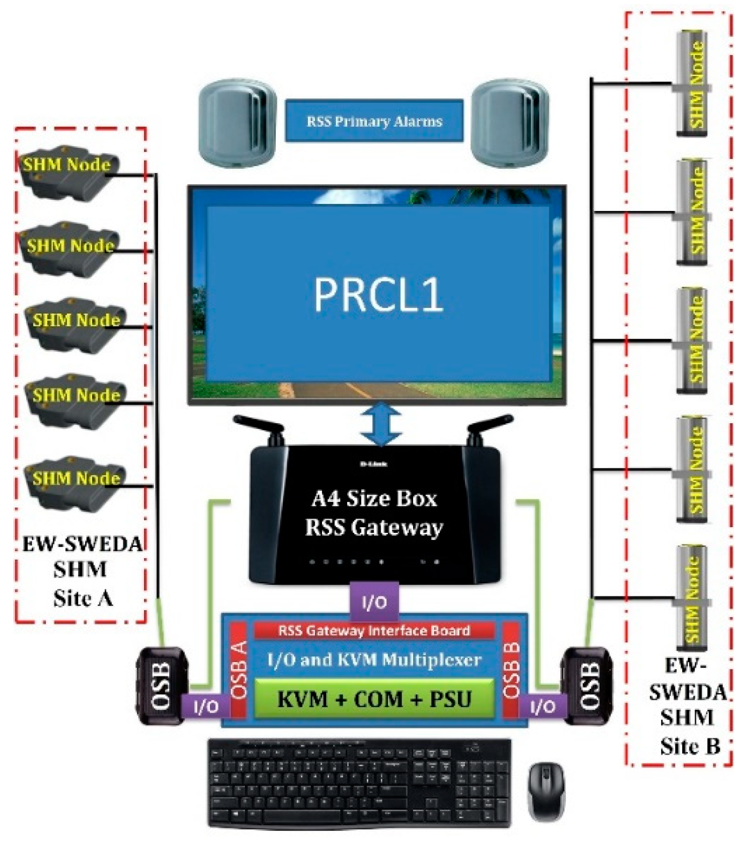
- SHM-QU-CO5-Bridge SWEDA-SHM Site (SHM-BS) System with 5 F-SGBINs.
- SHM-QU-B09-Lab SWEDA-SHM site (SHM-LB) with 5 F-SGBINs and 10 C-SGBINs.
- SGBINs placement anomalies, i.e., all sensors were not symmetric neither vertically nor horizontally.
- SGBINs output contained unwanted amplitudes and frequencies that were increasing the computation costs as well as false detection.
- The early warning estimation was a major challenge, i.e., the requirement of peak detection or extremities in the signal.
- The seismic waves automated recording and processing activation needed unique peaks and frequencies identification.
- The seismic waves runtime similarities estimation with an expected earthquake or seismic signal needed magnitude ratios as well as signal clustering.
- The STA/LTA triggering only for featured events was a mandatory step that had to be performed.
- A probabilistic sequence for an earthquake for runtime conditions was also needed for the next or upcoming signals similarity assessment.
- Sending a new sampling scheme for the optimization of ADC was also needed to only capture the needed signals and reduce the post-analysis costs.
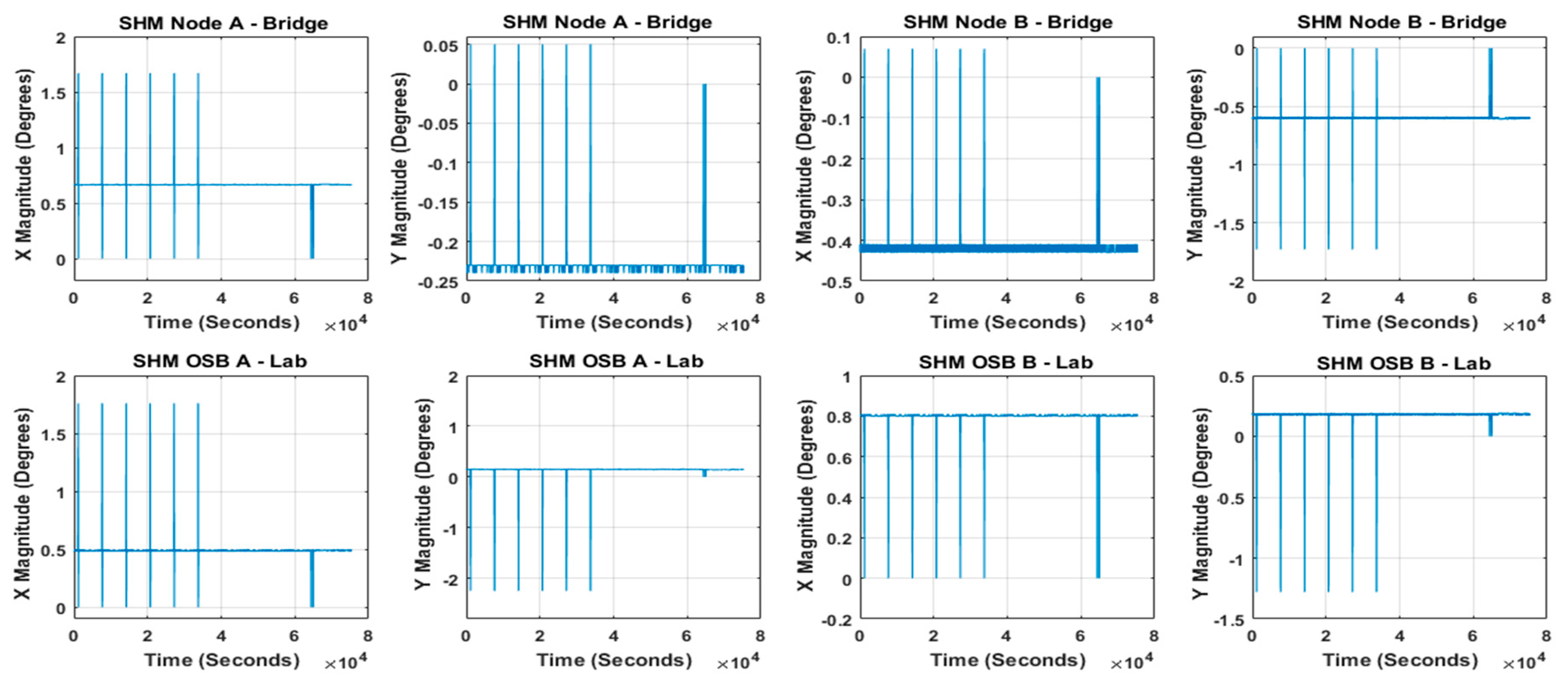
5. Results
6. Discussion and Limitations
6.1. The Problem/Challenge
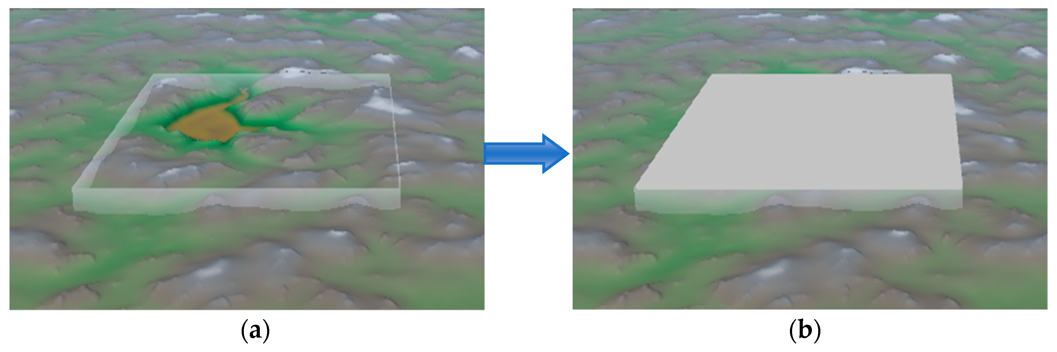
- Which surface is suitable for seismic wave detection?
- Which sensors are best for ground motion frequency, magnitude, and angle measurement?
- How to align the crust or surface with sensors for ground motion detection?
- How to reduce the computation by minimizing mathematical complexity?
- How to detect if the disaster threshold is exceeded for the early warning?
- How does the data need to be filtered for feature extraction and pattern recognition?
- How to relate the curves that they can be decisive evidence of the seismic event?
- What is the probability of an earthquake?
- Which data structure is more suitable for the real-time accuracy of prediction?
- What are the recommended specifications of the sensor resolution ideal for SWEDA?
- What should be the communication configuration of urban-scale seismic sensor nodes for an efficient algorithmic response?
6.2. The Contribution of Proposed SWEDA Application on SGBINs
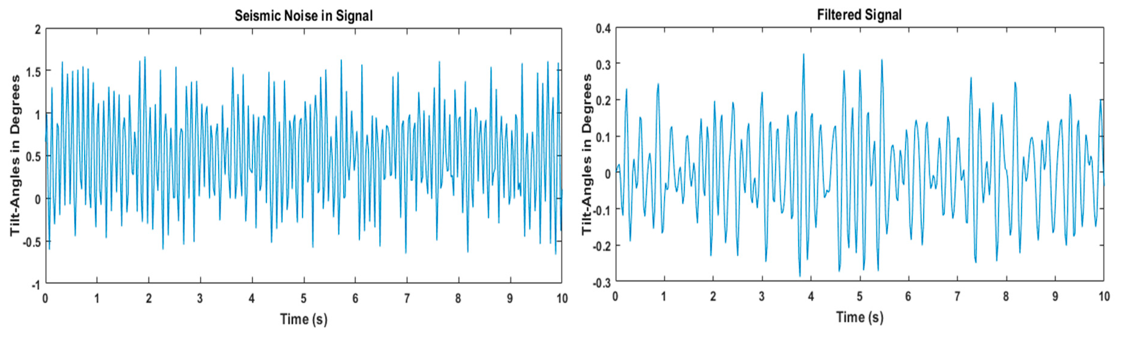
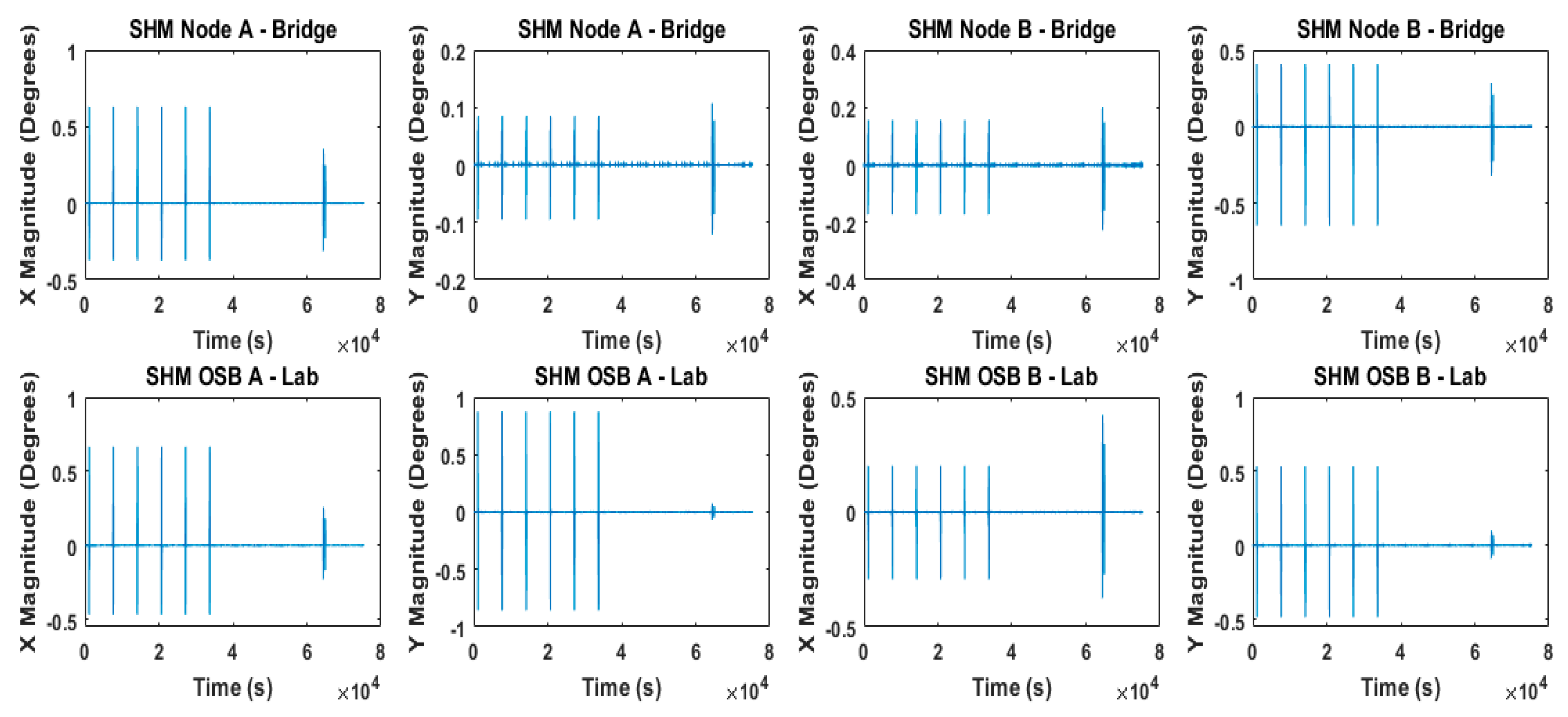
- Step 2: All the SGBIN SP1s outputs were filtered by SNF (Figure 21) using a MicroPython embedded filter signal. The savgol_filter eliminated unwanted frequencies by only allowing a range of 1~24 Hz. Furthermore, the ranges of more than ±5° amplitudes were eliminated, which were increasing the computation costs as well as directing towards false detection.
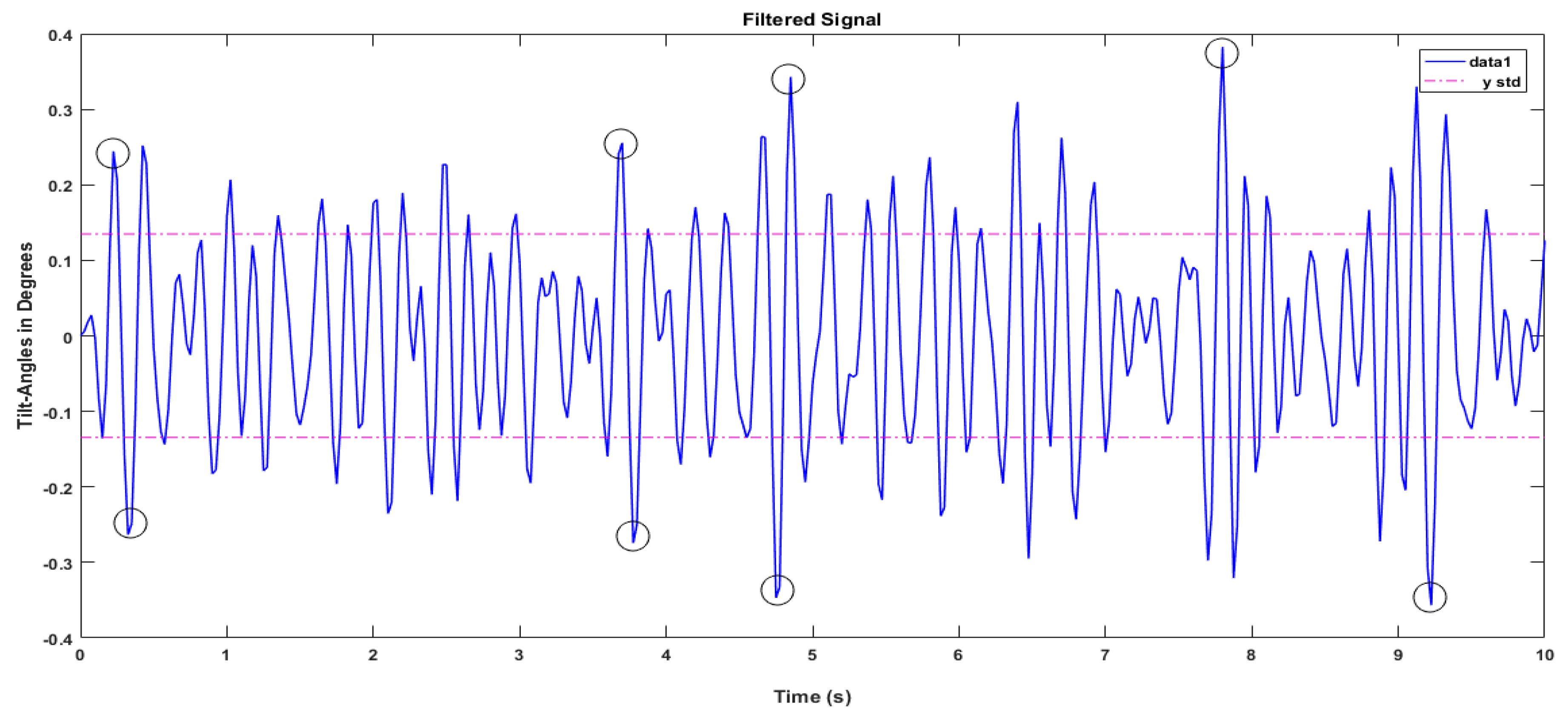
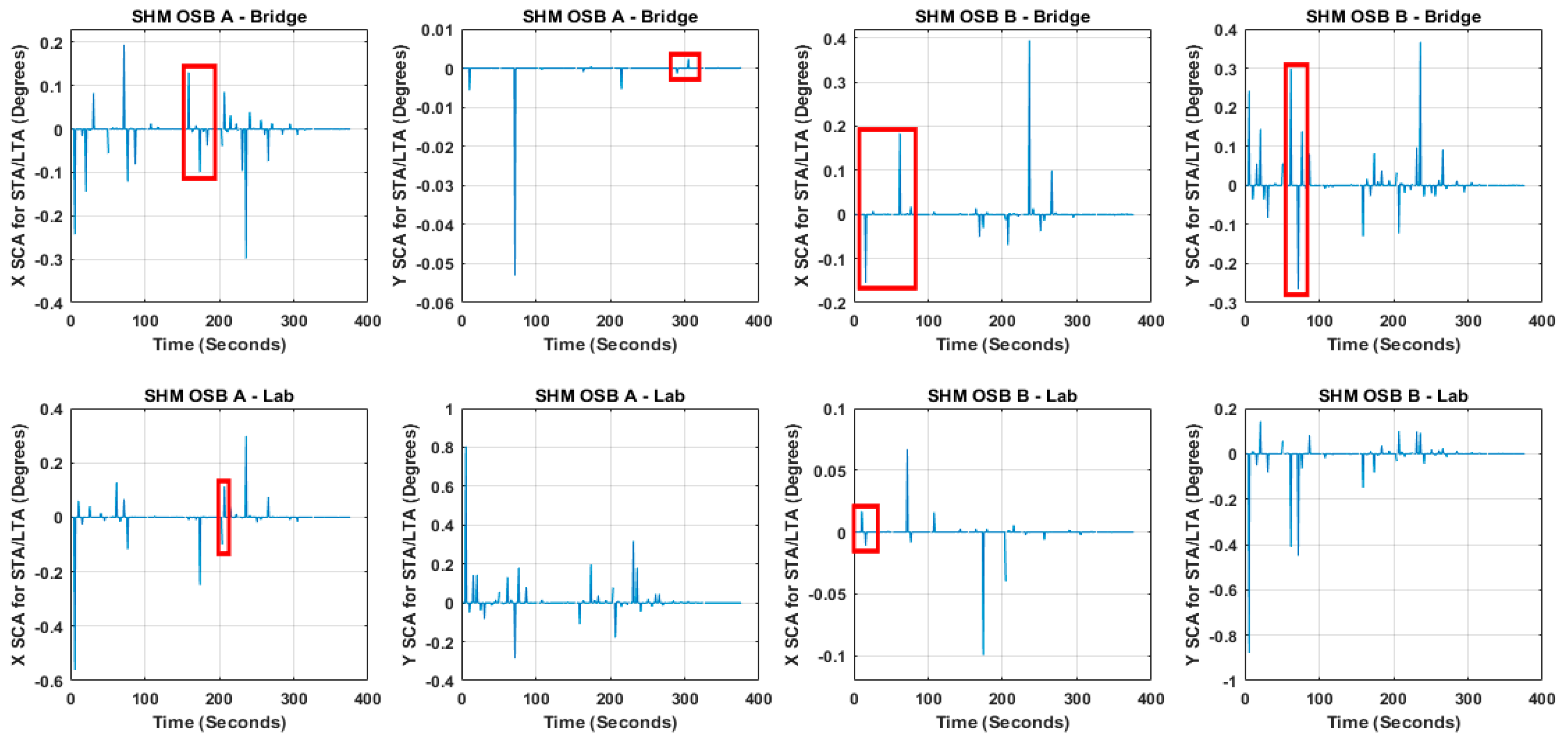
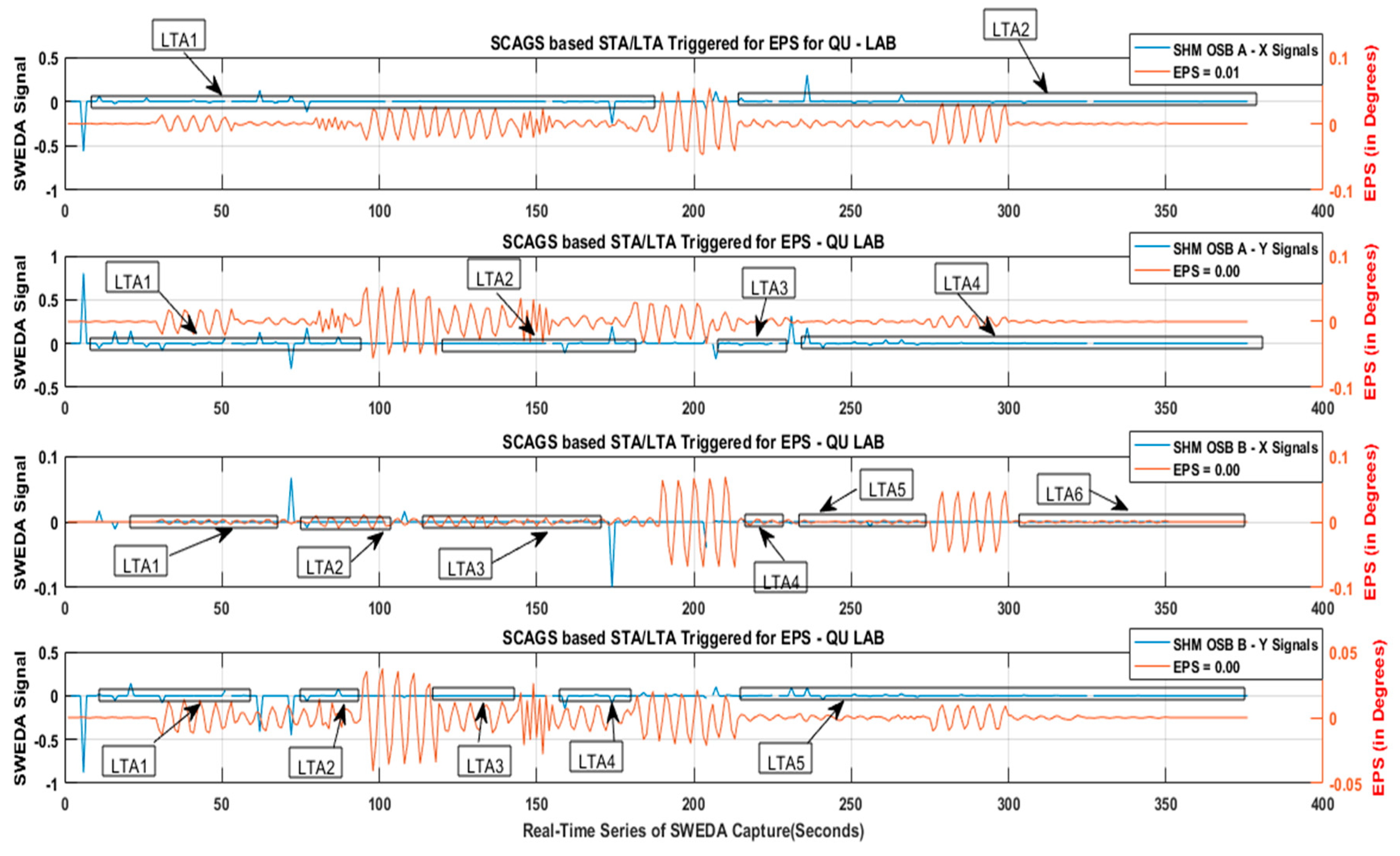
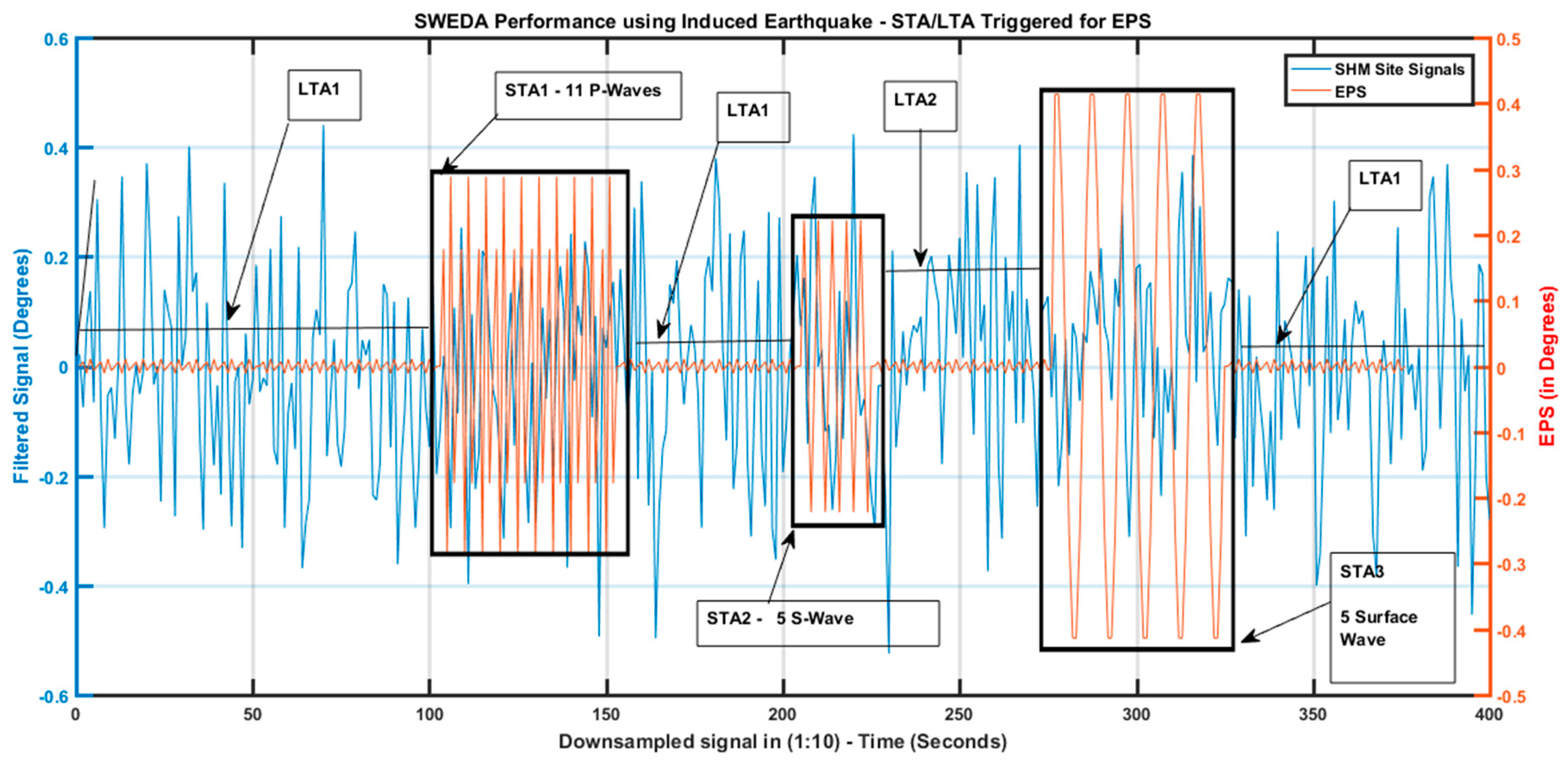
- Step 4: The unique peak detection operation generated SCAGS and triggering amplitudes for STA/LTA in SLAWS for a stationary signal, as no seismic conditions were observed by PDS in Figure 22.
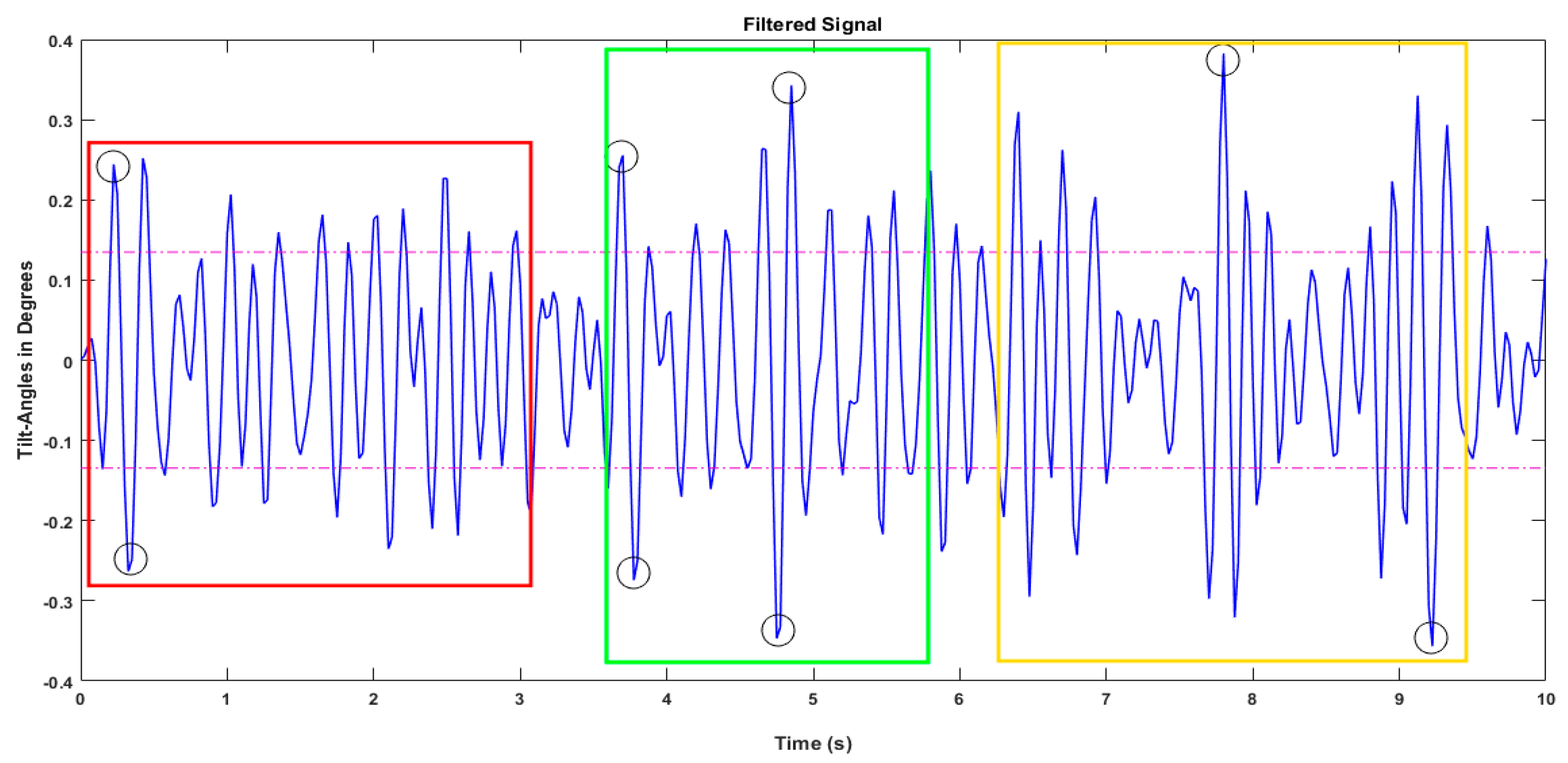
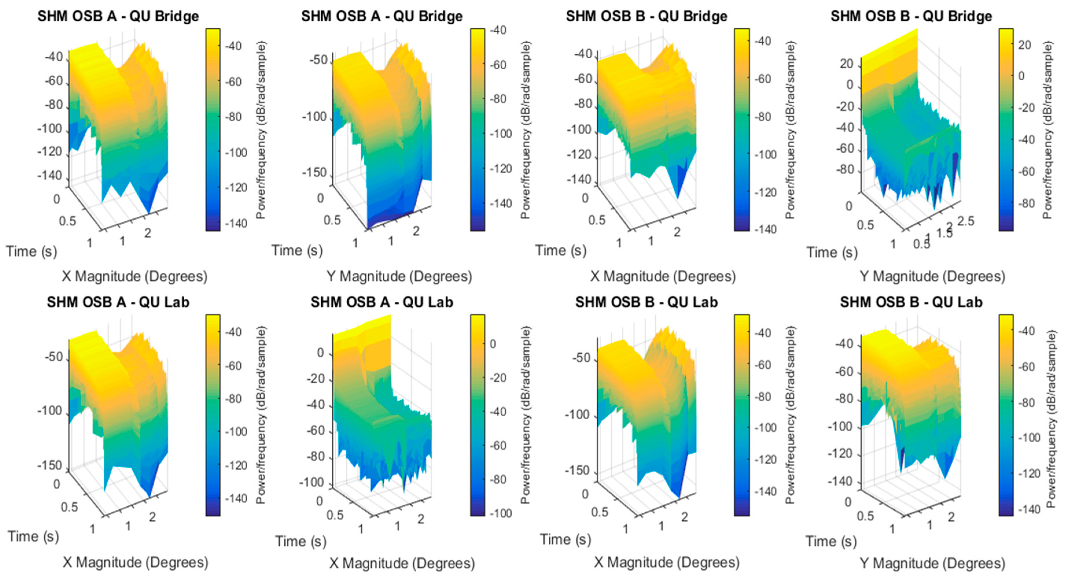
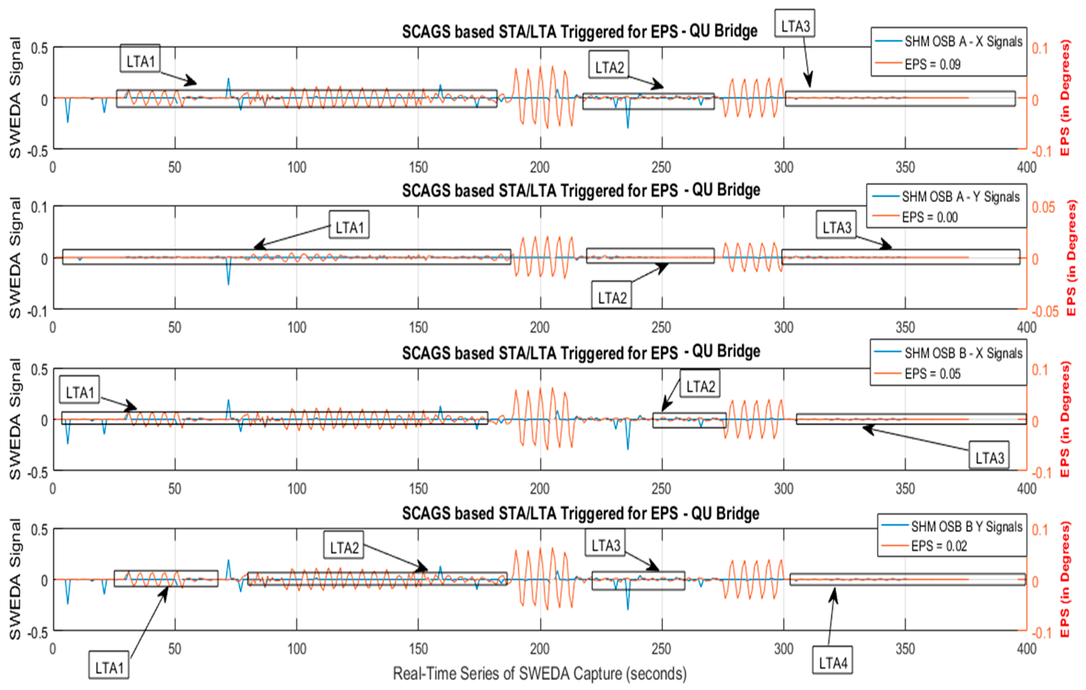
- Step 5: The runtime similarities estimation using ratio computation with SCAGS and SLAWS generated an EPS for an expected earthquake or seismic signal needed magnitude ratios as well as the signal clustering, presented in Figure 23 as the green gradient.
- The limitation of this work in the implementation phase is a dependency on proposed SGBINs.
- The sequence of operations has to be observed in the same pattern.
7. Future Recommendations
8. Conclusions
Author Contributions
Funding
Conflicts of Interest
References
- Herlander, M.; Andreilcy, A.; Adilson, P.; Abel, M.; José, A.A. Impacts of Natural Disasters on Environmental and Socio-Economic Systems: What makes the difference? Ambiente Soc. 2013, 16, 45–64. [Google Scholar]
- Franco, A.; Peter, N.; Frits, J.S. The Challenge of Sustainable Development. In Economy and Ecology: Towards Sustainable Development. Economy & Environment; Springer: Dordrecht, The Netherlands, 1989. [Google Scholar]
- Mario, A.R.E.; Donghyun, P. A New Assessment to Measure the Risk Levels between Natural Disasters and Socio- Economic-Political Disasters. Available SSRN 3400582 2019. [Google Scholar] [CrossRef]
- Wenzhan, S.; Fangyu, L.; Maria, V.; Liang, Z. Toward Creating a Subsurface Camera. Sensors 2019, 19, 301. [Google Scholar]
- Abdurrahman, S.; Rafet, S.; Aysegul, A.; Muneo, H. Development of Integrated Earthquake Simulation System for Istanbul. Earth Planets Space 2016, 68, 115. [Google Scholar]
- Hasan, T.; Farid, T.; Damiano, C.; Adel, B.M. Design and Implementation of Programmable Multi-Parametric 4-Degrees of Freedom Seismic Waves Ground Motion Simulation IoT Platform. In Proceedings of the Fifteenth International Wireless Communications & Mobile Computing Conference (IWCMC), Tangier, Morocco, 24–28 June 2019. [Google Scholar]
- Öcal, N. Design and Challenges for a Tsunami Early Warning System in the Marmara Sea. Earth Planets Space 2016, 68, 13. [Google Scholar]
- Christelle, S.; Pierre-Yves, B.; Bertrand, G.; Jacques, H.; Cécile, C.; Jocelyne, G.; Michelle, A. Using Ambient Vibration Measurements for Risk Assessment at an Urban Scale: From Numerical Proof of Concept to Beirut Case Study (Lebanon). Earth Planets Space 2017, 69, 60. [Google Scholar]
- Hasan, T.; Anas, T.; Farid, T.; Mohammed, A.A.; Adel, B.M.; Damiano, C. Geographical Area Network—Structural Health Monitoring Utility Computing Model. Int. J. Geo Inf. 2018, 8, 154. [Google Scholar]
- Ware, R.H.; Fulker, D.W.; Stein, S.A.; Anderson, D.N.; Avery, S.K.; Clark, R.D.; Droegemeier, K.K.; Kuettner, J.P.; Minster, J.; Sorooshian, S. Real-time National GPS Networks: Opportunities for Atmospheric Sensing. Earth Planets Space 2019, 52, 901–905. [Google Scholar] [CrossRef]
- Arvid, H. Civil Structural Health Monitoring Strategies, Methods and Applications. Ph.D. Thesis, Luleå Tekniska Universitet, Luleå, Sweden, 2007. [Google Scholar]
- Farid, T.; Hasan, T.; Mohammed, A.A.; Adel, B.M.; Damiano, C. Design and Simulation of a Green Bi-Variable Mono-Parametric SHM Node and Early Seismic Warning Algorithm for Wave Identification and Scattering. In Proceedings of the 14th International Wireless Communications & Mobile Computing Conference (IWCMC), Limassol, Cyprus, 25–29 June 2018. [Google Scholar] [CrossRef]
- Farid, T.; Hasan, T.; Mohammed, A.A.; Adel, B.M.; Anas, T.; Damiano, C. IoT and IoE prototype for scalable infrastructures, architectures and platforms. Int. Robot. Autom. J. 2018. [Google Scholar] [CrossRef]
- Farid, T.; Hasan, T.; Adel, B.M.; Damiano, C. Development of Prototype for IoT and IoE Scalable Infrastructures, Architectures and Platforms. In Proceedings of the Fourth International Symposium, Ubiquitous Networking, Hammamet, Tunisia, 2–5 May 2018. [Google Scholar] [CrossRef]
- Eric, N.H.; Mohammed, S.H. Gator: An Optimized Discrimination Network for Active Database Rule Condition Testing. Master’s Thesis, CIS Department University of Florida, Gainesville, FL, USA, 1993. [Google Scholar]
- Hasan, T.; Anas, T.; Farid, T.; Mohammed, A.A.; Adel, B.M.; Damiano, C. Structural Health Monitoring Installation and Deployment Scheme using Utility Computing Model. In Proceedings of the Second European Conference in EECS, Bern, Switzerland, 20–22 December 2018. [Google Scholar]
- Mohammad, A.H.; Mohammad, K.H.; Pin, J.K.H. A review on sensors and systems in structural health monitoring: Current issues and challenges. Smart Struct. Syst. 2018, 22, 509–525. [Google Scholar]
- Arvind, D.; Ali, D.; Chun, H.W.; Sabu, J. A Review of Passive Wireless Sensors for Structural Health Monitoring. Mod. Appl. Sci. 2013, 7, 57–76. [Google Scholar]
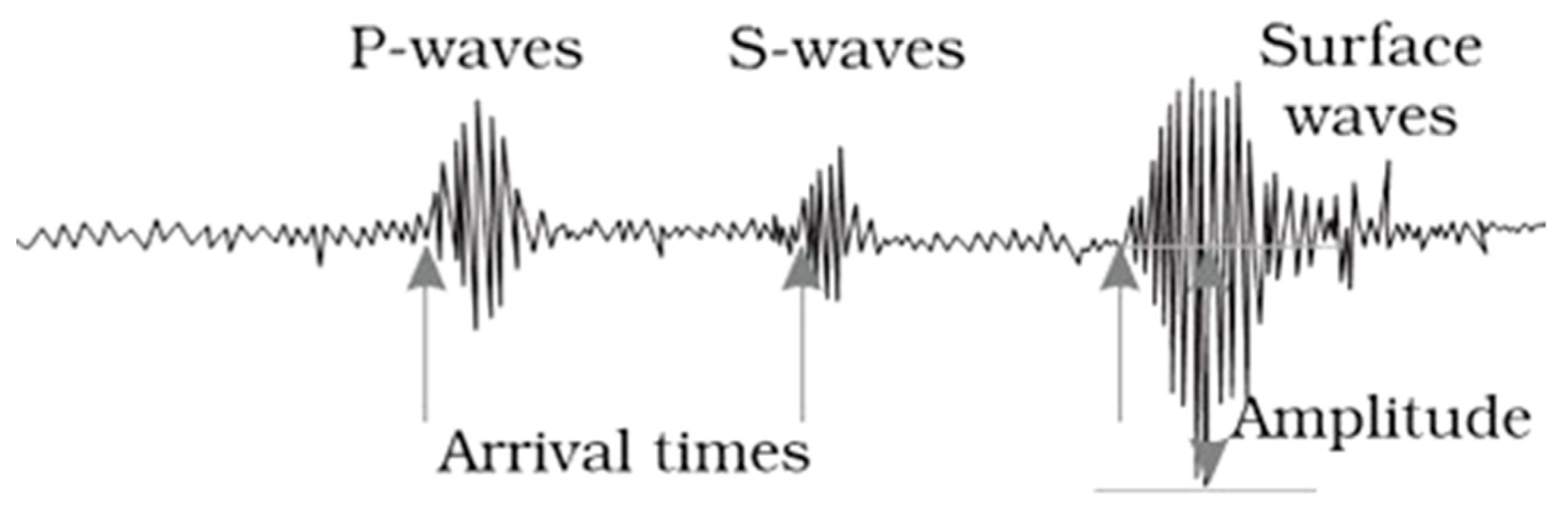
- Maria, L.; Aldo, Z. A Bayesian Approach to the Real-time Estimation of Magnitude from the Early P and S Wave Displacement Peaks. J. Geophys. Res. Atmos. 2008. [Google Scholar] [CrossRef]
- Wu, H.; Zhang, B.; Li, F.; Liu, N. Semi-automatic first arrival picking of micro-seismic events by using pixel-wise convolutional image segmentation. Geophysics 2019, 84, V143–V155. [Google Scholar] [CrossRef]
- Zefeng, L.; Men-Andrin, M.; Egill, H.; Zhongwen, Z.; Jennifer, A. Machine Learning Seismic Wave Discrimination: Application to Earthquake Early Warning. Geophys. Res. Lett. 2018, 45, 4773–4779. [Google Scholar]
- Ioannis, A.; Ioannis, T.; Anaxagoras, E. Intelligent Seismic Acceleration Signal Processing for Damage Classification in Buildings. IEEE Trans. Instrum. Meas. 2007, 56, 1555–1564. [Google Scholar]
- Niksa, O.; Sven, L. Earthquake-explosion Discrimination using Genetic Algorithm based Boosting Approach. Comput. Geosci. 2010, 36, 179–185. [Google Scholar]
- Conny, H.; Moritz, B.; Matthias, O. A seismic event spotting system for volcano fast response systems. Bull. Seismol. Soc. Am. 2012, 102, 948–960. [Google Scholar]
- Silvia, S.F.; Eugène, C.E.; Mohammad, I.M. Automatic Classification of Seismic Signals at Mt. Vesuvius Volcano, Italy, using Neural Networks. Bull. Seismol. Soc. Am. 2005, 95, 185–196. [Google Scholar]
- Cheng, T.; Brian, L.N.K. Automatic Seismic Event Recognition and Later Phase Identification for Broadband Seismograms. Bull. Seismol. Soc. Am. 2009, 86, 1896–1909. [Google Scholar]
- Claudio, S.; Yih-Min, W.; Aldo, Z.; Hiroo, K. Earthquake Early Warning: Concepts, Methods and Physical Grounds. Soil Dyn. Earthq. Eng. 2011, 31, 106–118. [Google Scholar]
- Jiang, W.; Yu, H.; Li, L.; Huang, L. A Robust Algorithm for Earthquake Detector. In Proceedings of the World Congress on Engineering Education (WCEE), Beirut, Lebanon, 29–30 October 2015. [Google Scholar]
- Mitchell, W.; Richard, A.; Christopher, Y.; Judy, B.; Mark, H.; Susan, M.; Julian, T. A Comparison of Select Trigger Algorithms for Automated Global Seismic Phase and Event Detection. Bull. Seismol. Soc. Am. 1998, 88, 95–106. [Google Scholar]
- Satish, K.; Renu, V.; Pawan, K. Development of Earthquake Event Detection Technique Based on STA/LTA Algorithm for Seismic Alert System. Geo. Soc. India 2018, 92, 679–686. [Google Scholar]
- Joshua, P.J.; Mirko, B. Adaptive STA–LTA with Outlier Statistics. Bull. Seismol. Soc. Am. 2015, 105, 1606–1618. [Google Scholar]
- Fangyu, L. Automatic Arrival Identification System for Real-time Microseismic Event Location. In Proceedings of the SEG International Exposition and 87th Annual Meeting, Houston, TX, USA, 24–27 September 2017. [Google Scholar]
- Fangyu, L.; Jamie, R.; Kurt, J.M.; Huailai, Z. Automatic event detection on noisy microseismograms. In Proceedings of the 84th Annual International Meeting, SEG, Expanded Abstracts, Las Vegas, NV, USA, 5 August 2014. [Google Scholar]
- Anthony, L.; Claudio, S.; Maurizio, V. Automatic Picker Developments and Optimization: FilterPicker—A Robust, Broadband Picker for Real-time Seismic Monitoring and Earthquake Early-Warning. Seismol. Res. Lett. 2012, 83, 531–540. [Google Scholar]
- Ruano, A.E.; Madureira, G.; Barros, O. Seismic Detection using Support Vector Machines. J. Neurocomputing 2013, 135, 273–283. [Google Scholar] [CrossRef]
- Serdar, K.H.; Richard, M.A.; Holly, B.; Margaret, H.; Ivan, H.; Douglas, N. Designing a Network-Based Earthquake Early Warning Algorithm for California: ElarmS-2. Bull. Seismol. Soc. Am. 2013, 104, 162–173. [Google Scholar] [CrossRef]
- Jubran, A.; David, W.E. A review and appraisal of arrival-time picking methods for downhole microseismic data. Geophysics 2016, 81, KS71–KS91. [Google Scholar]
- Thomas, B.; Mike, E.D. Normalized Iterative Hard Thresholding: Guaranteed Stability and Performance. Ieee J. Sel. Top. Signal. Process. 2009, 4, 298–309. [Google Scholar]
- Jonathan, B.; Jonathan, M.B. Two-point step size gradient methods. IMA J. Numer. Anal. 1998, 8, 141–148. [Google Scholar]
- Sleeman, T.; Torild, V.E. Robust automatic P-phase picking: An on-line implementation in the analysis of broadband seismogram recordings. Phys. Earth Planet. Int. 1999, 113, 265–275. [Google Scholar] [CrossRef]
- Dias, P.J.M.; Postolache, O.; Girão, P.M. Digitally Programmable A/D Converter for Smart Sensors Applications. IEEE Trans. Instrum. Meas. 2017, 56, 158–163. [Google Scholar] [CrossRef]
- Peter, J.; Cees, V.L. OMPC: An Open-Source MATLAB-to-Python Compiler. Front. Neuroinformatics 2007, 3, 5. [Google Scholar]
- Masatoshi, M. Detection of seismic events triggered by P-waves from the 2011 Tohoku-Oki earthquake. Earth Planets Space 2013, 64, 16. [Google Scholar]
- Lucia, M.; Leif, W.; John, B. A Comparison of Coda and S-Wave Spectral Ratios as Estimates of Site Response in the Southern San Francisco Bay Area. Bull. Seismol. Soc. Am. 1994, 84, 1815–1830. [Google Scholar]
- Fan-Chi, L.; Morgan, P.M.; Michael, H.R. Surface wave Tomography of the Western United States from Ambient Seismic Noise: Rayleigh and Love wave Phase Velocity Maps. Geophys. J. Int. 2007, 173, 281–298. [Google Scholar]


| Algorithms | Computational Cost | Floating-Point Operations |
|---|---|---|
| Hamming Windowing | M | 1.440 |
| Fast Fourier Transform (FFT) | NA * log2(NA) | 22.528 |
| (abs)2 | NA/2 | 10.24 |
| Filter Bank | NA/2 * Rfb | 49.152 |
| Logarithm | Rfb | 48 |
© 2019 by the authors. Licensee MDPI, Basel, Switzerland. This article is an open access article distributed under the terms and conditions of the Creative Commons Attribution (CC BY) license (http://creativecommons.org/licenses/by/4.0/).
Share and Cite
Tariq, H.; Touati, F.; E. Al-Hitmi, M.A.; Crescini, D.; Ben Mnaouer, A. A Real-Time Early Warning Seismic Event Detection Algorithm Using Smart Geo-Spatial Bi-Axial Inclinometer Nodes for Industry 4.0 Applications. Appl. Sci. 2019, 9, 3650. https://doi.org/10.3390/app9183650
Tariq H, Touati F, E. Al-Hitmi MA, Crescini D, Ben Mnaouer A. A Real-Time Early Warning Seismic Event Detection Algorithm Using Smart Geo-Spatial Bi-Axial Inclinometer Nodes for Industry 4.0 Applications. Applied Sciences. 2019; 9(18):3650. https://doi.org/10.3390/app9183650
Chicago/Turabian StyleTariq, Hasan, Farid Touati, Mohammed Abdulla E. Al-Hitmi, Damiano Crescini, and Adel Ben Mnaouer. 2019. "A Real-Time Early Warning Seismic Event Detection Algorithm Using Smart Geo-Spatial Bi-Axial Inclinometer Nodes for Industry 4.0 Applications" Applied Sciences 9, no. 18: 3650. https://doi.org/10.3390/app9183650
APA StyleTariq, H., Touati, F., E. Al-Hitmi, M. A., Crescini, D., & Ben Mnaouer, A. (2019). A Real-Time Early Warning Seismic Event Detection Algorithm Using Smart Geo-Spatial Bi-Axial Inclinometer Nodes for Industry 4.0 Applications. Applied Sciences, 9(18), 3650. https://doi.org/10.3390/app9183650