Restricted Boltzmann Machine Vectors for Speaker Clustering and Tracking Tasks in TV Broadcast Shows †


Abstract
1. Introduction
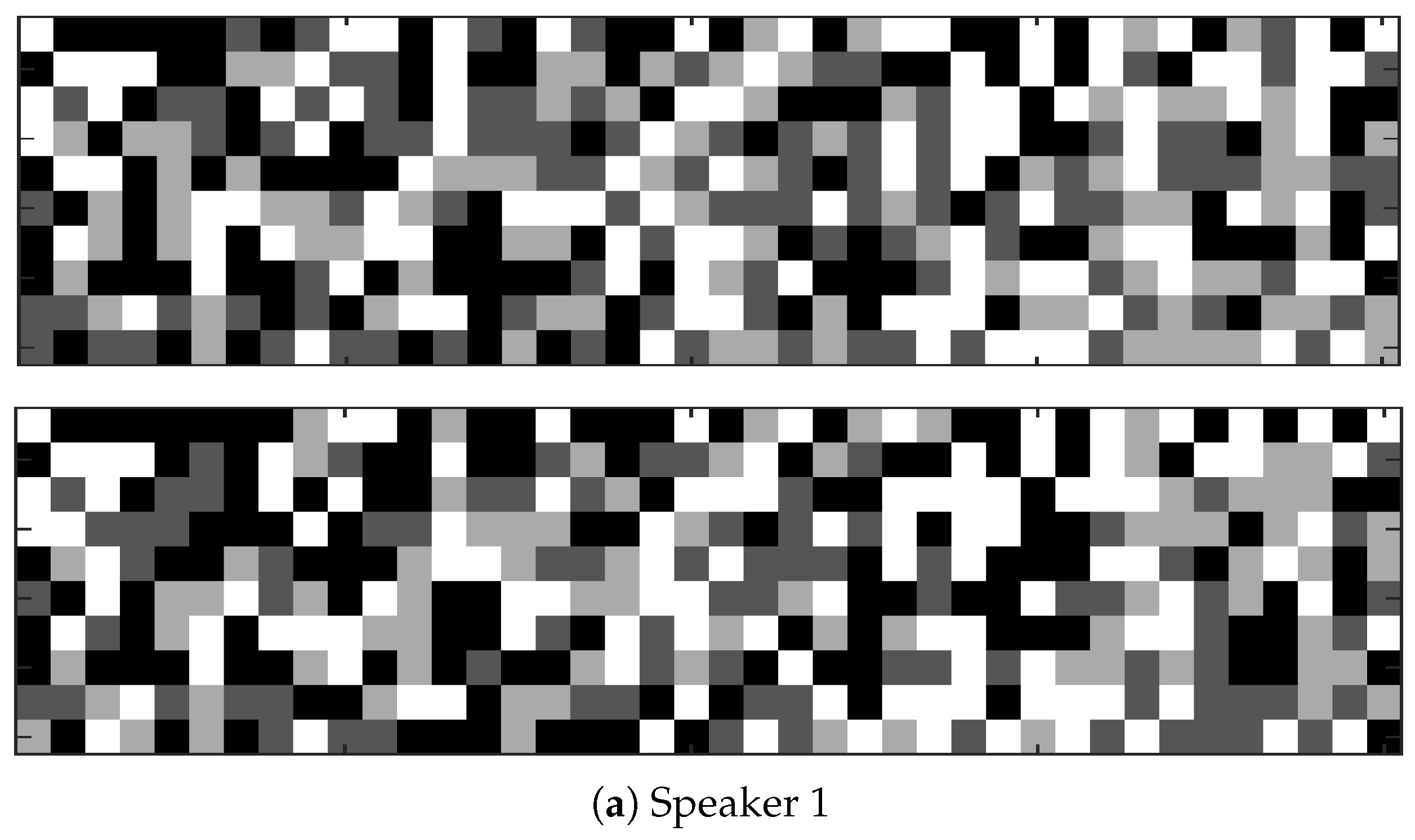
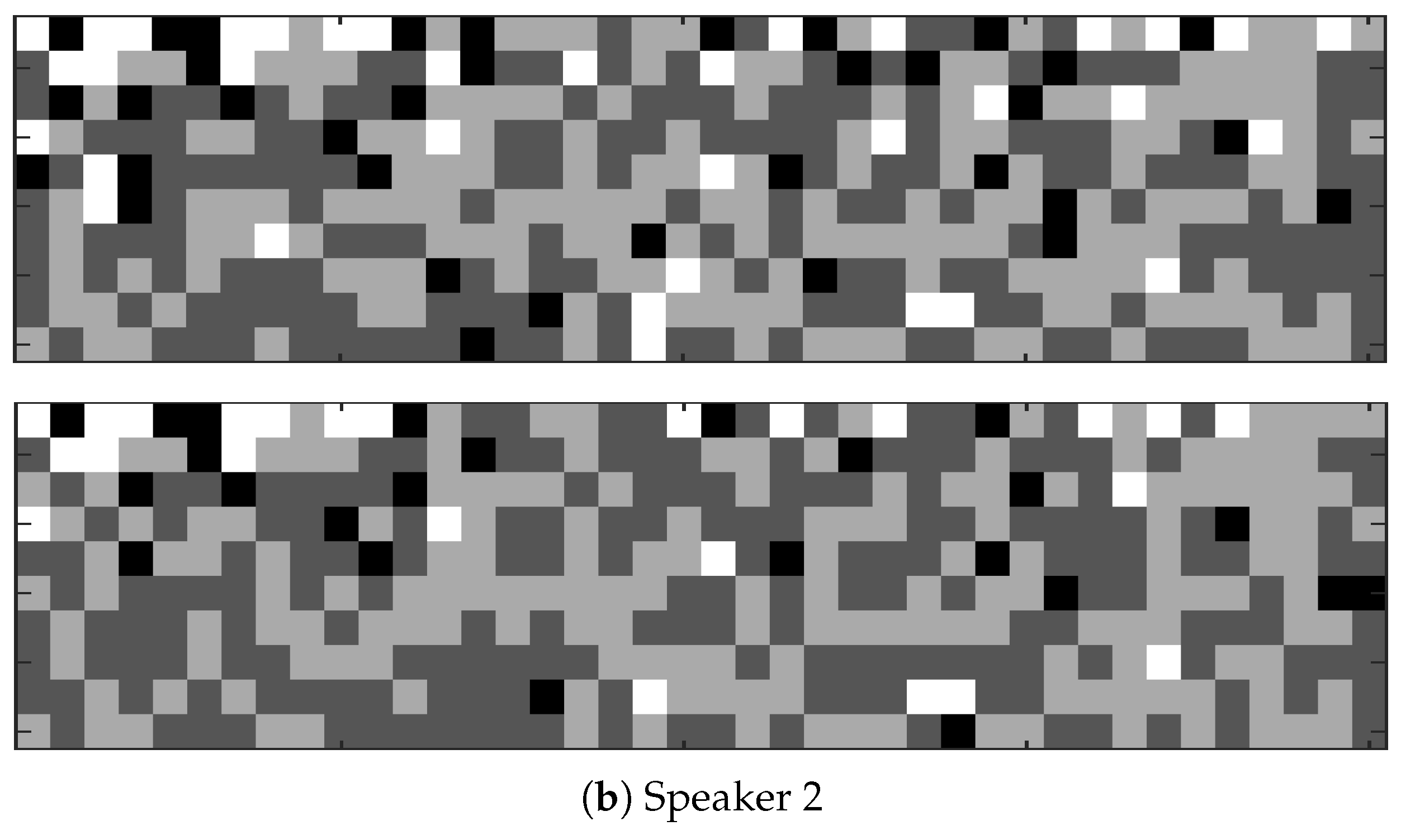
2. RBM Vector Representation
2.1. URBM Training
2.2. RBM Adaptation
2.3. RBM Vector Extraction
3. Speaker Clustering
- (a)
- Average Linkage:
- (b)
- Single Linkage:where is the score between new cluster and old segment while is the score between old segments and .
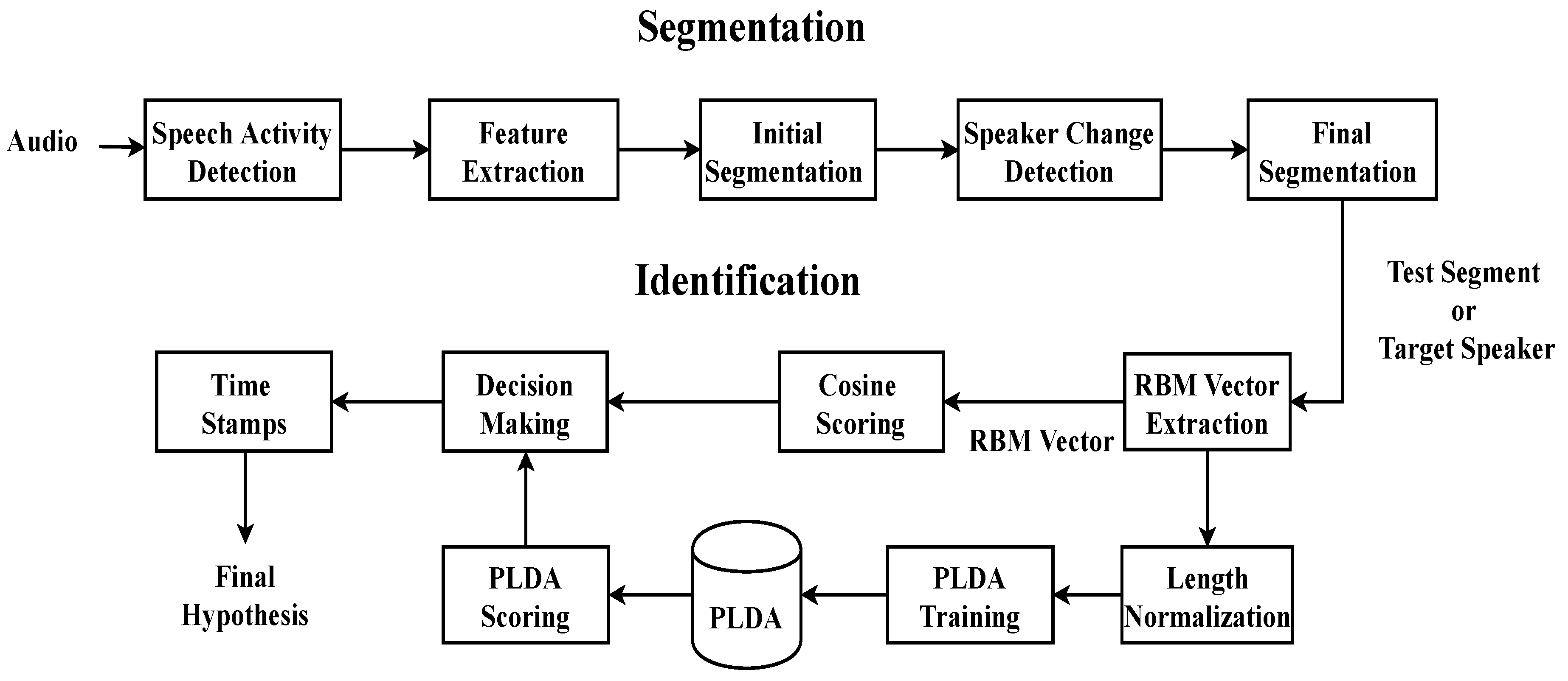
4. Speaker Tracking
4.1. Speaker Segmentation
4.2. Speaker Identification
5. Experimental Setup and Database
5.1. Database
5.2. Baseline and RBM Vector Setup
5.3. Evaluation Metrics
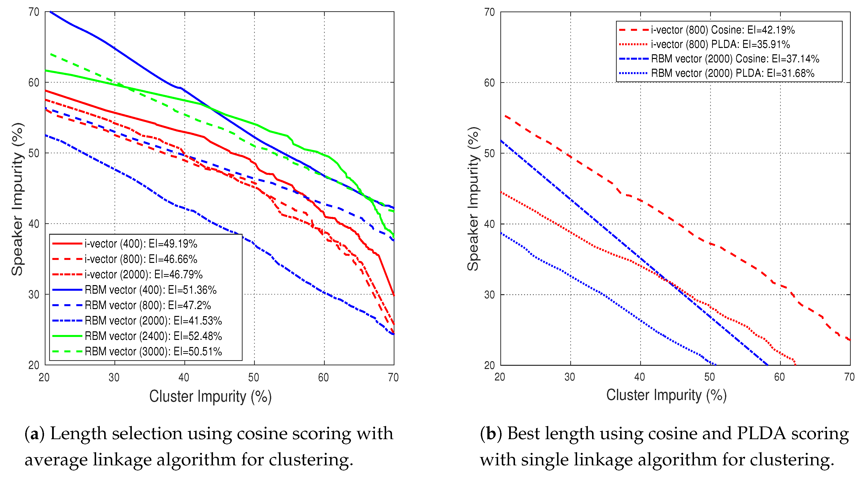
6. Results
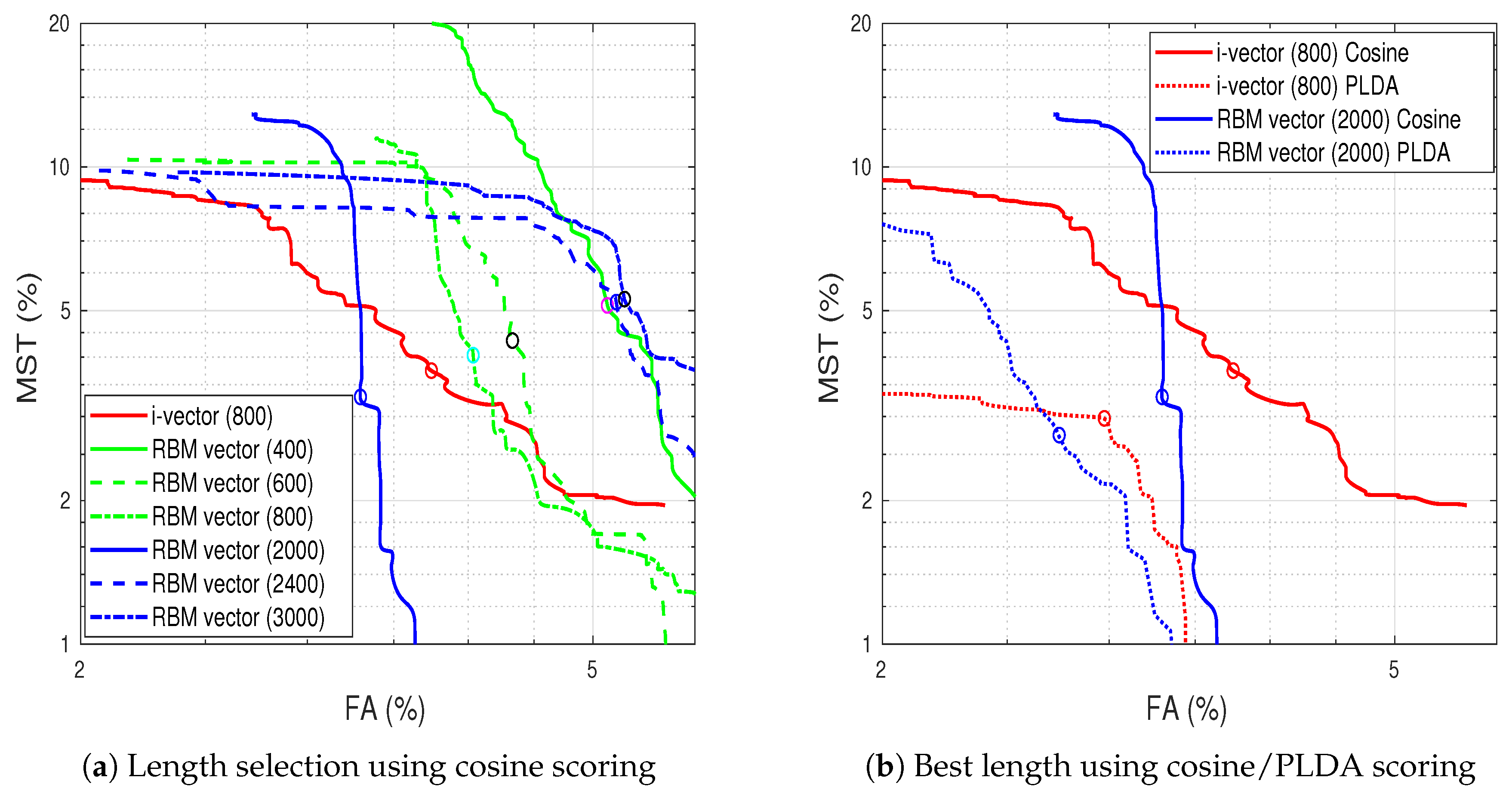
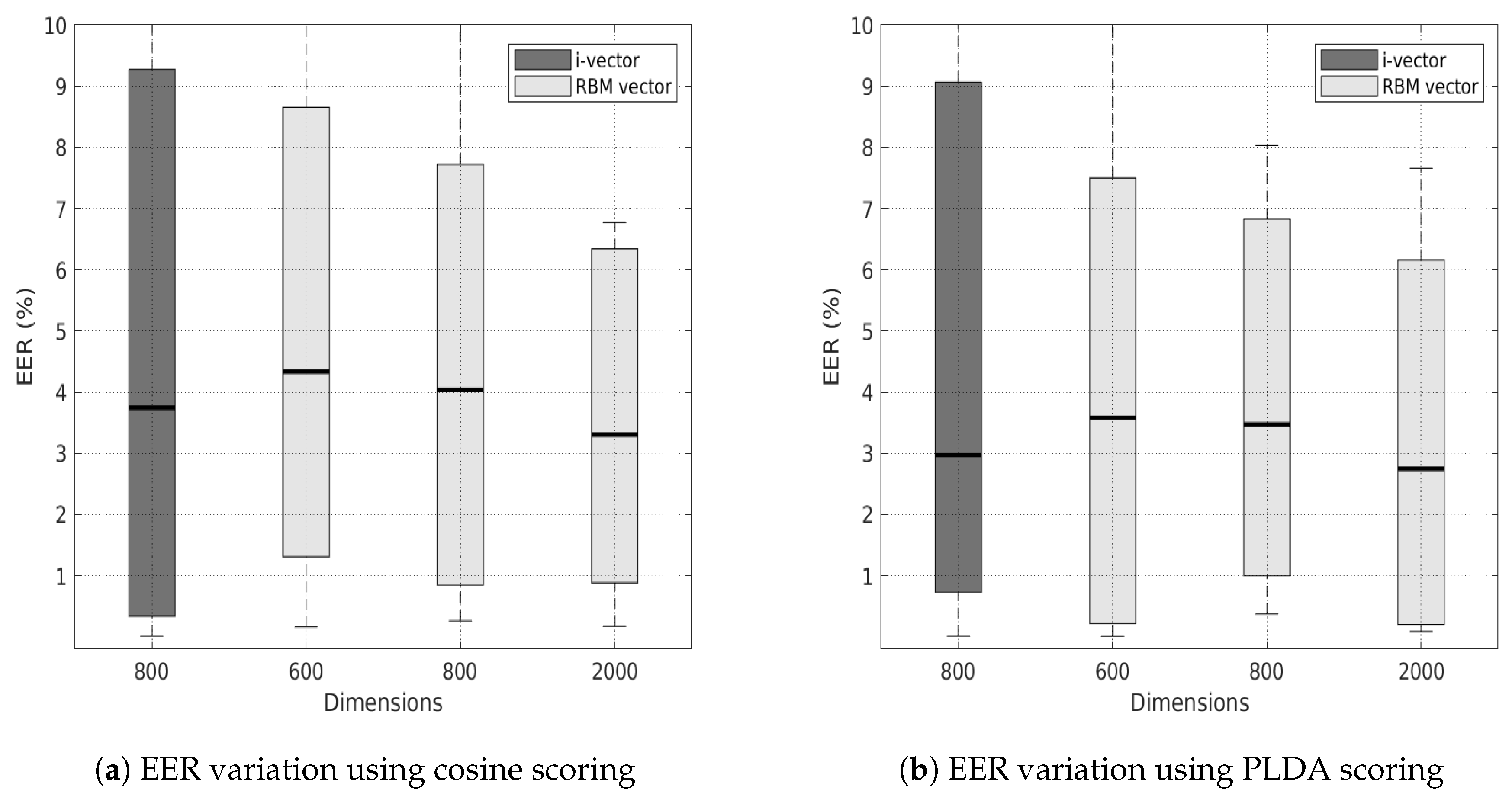
6.1. Speaker Clustering
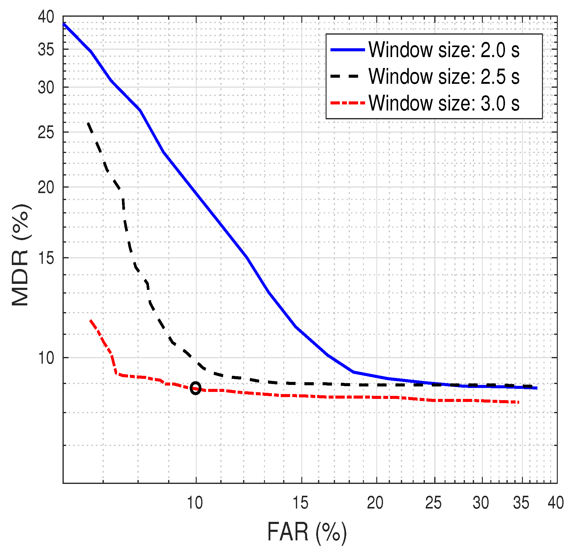
6.2. Speaker Tracking
7. Conclusions
Author Contributions
Funding
Conflicts of Interest
Abbreviations
| RBM | Restricted Boltzmann Machines |
| EI | Equal Impurity |
| PLDA | Probabilistic Linear Discriminant Analysis |
| GMM | Gaussian Mixture Models |
| HMM | Hidden Markov Models |
| DNN | Deep Neural Networks |
| DBN | Deep Belief Networks |
| BNF | Bottle Neck Features |
| AHC | Agglomerative Hierarchical Clustering |
| PCA | Principal Component Analysis |
| URBM | Universal Restricted Boltzmann Machines |
| MVN | Mean Variance Normalized |
| CD | Contrastive Divergence |
| SAD | Speech Activity Detection |
| MFCC | Mel-Frequency Cepstral Coefficients |
| UBM | Universal Background Model |
| TV | Total Variability |
| CI | Cluster Impurity |
| SI | Speaker Impurity |
| IT | Impurity Trade-off |
| FA | False Alarm |
| MST | Missed Speaker time |
| FAR | False Alarm Rate |
| MDR | Miss Detection Rate |
| DET | Detection Error Trade-off |
References
- Lei, Y.; Scheffer, N.; Ferrer, L.; McLaren, M. A novel scheme for speaker recognition using a phonetically-aware deep neural network. In Proceedings of the IEEE International Conference on Acoustics, Speech and Signal Processing (ICASSP), Florence, Italy, 4–9 May 2014; pp. 1695–1699. [Google Scholar]
- Richardson, F.; Reynolds, D.; Dehak, N. Deep neural network approaches to speaker and language recognition. IEEE Signal Process. Lett. 2015, 22, 1671–1675. [Google Scholar] [CrossRef]
- Chen, K.; Salman, A. Learning speaker-specific characteristics with a deep neural architecture. IEEE Trans. Neural Netw. 2011, 22, 1744–1756. [Google Scholar] [CrossRef] [PubMed]
- Kenny, P.; Gupta, V.; Stafylakis, T.; Ouellet, P.; Alam, J. Deep neural networks for extracting baum-welch statistics for speaker recognition. Proc. Odyssey 2014, 293–298. Available online: https://www.isca-speech.org/archive/odyssey_2014/pdfs/28.pdf (accessed on 8 July 2019).
- Liu, Y.; Qian, Y.; Chen, N.; Fu, T.; Zhang, Y.; Yu, K. Deep feature for text-dependent speaker verification. Speech Commun. 2015, 73, 1–13. [Google Scholar] [CrossRef]
- Deng, L.; Yu, D. Deep learning: Methods and applications. Found. Trends Signal Process. 2014, 7, 197–387. [Google Scholar] [CrossRef]
- Yamada, T.; Wang, L.; Kai, A. Improvement of distant-talking speaker identification using bottleneck features of DNN. Interspeech 2013, 3661–3664. Available online: https://www.isca-speech.org/archive/archive_papers/interspeech_2013/i13_3661.pdf (accessed on 8 July 2019).
- Lee, H.; Pham, P.; Largman, Y.; Ng, A.Y. Unsupervised feature learning for audio classification using convolutional deep belief networks. In Advances in Neural Information Processing Systems; Curran Associates, Inc., 2009; pp. 1096–1104. Available online: http://papers.nips.cc/paper/3674-unsupervised-feature-learning-for-audio-classification-using-convolutional-deep-belief-networks.pdf (accessed on 8 July 2019).
- Jorrín, J.; García, P.; Buera, L. DNN Bottleneck Features for Speaker Clustering. Proc. Interspeech 2017, 1024–1028. [Google Scholar] [CrossRef]
- Jati, A.; Georgiou, P. Speaker2Vec: Unsupervised Learning and Adaptation of a Speaker Manifold using Deep Neural Networks with an Evaluation on Speaker Segmentation. Proc. Interspeech 2017, 3567–3571. [Google Scholar] [CrossRef]
- Anna, S.; Lukáš, B.; Jan, C. Alternative Approaches to Neural Network Based Speaker Verification. Proc. Interspeech 2017, 1572–1575. [Google Scholar] [CrossRef]
- Variani, E.; Lei, X.; McDermott, E.; Moreno, I.L.; Gonzalez-Dominguez, J. Deep neural networks for small footprint text-dependent speaker verification. In Proceedings of the IEEE International Conference on Acoustics, Speech and Signal Processing (ICASSP), 2014; pp. 4052–4056. Available online: https://ieeexplore-ieee-org.recursos.biblioteca.upc.edu/stamp/stamp.jsp?tp=&arnumber=6854363 (accessed on 8 July 2019).
- Isik, Y.Z.; Erdogan, H.; Sarikaya, R. S-vector: A discriminative representation derived from i-vector for speaker verification. In Proceedings of the IEEE 23rd European Signal Processing Conference (EUSIPCO), Nice, France, 31 August–4 September 2015; pp. 2097–2101. [Google Scholar]
- Bhattacharya, G.; Alam, J.; Kenny, P. Deep Speaker Embeddings for Short-Duration Speaker Verification. Proc. Interspeech 2017, 1517–1521. [Google Scholar] [CrossRef]
- Gong, Y. Speech recognition in noisy environments: A survey. Speech Commun. 1995, 16, 261–291. [Google Scholar] [CrossRef]
- Siniscalchi, S.M.; Salerno, V.M. Adaptation to new microphones using artificial neural networks with trainable activation functions. IEEE Trans. Neural Netw. Learn. Syst. 2016, 28, 1959–1965. [Google Scholar] [CrossRef]
- Huang, G.; Huang, G.B.; Song, S.; You, K. Trends in extreme learning machines: A review. Neural Netw. 2015, 61, 32–48. [Google Scholar] [CrossRef] [PubMed]
- Khoo, S.; Man, Z.; Cao, Z. Automatic han chinese folk song classification using extreme learning machines. In Australasian Joint Conference on Artificial Intelligence; Springer: Berlin/Heidelberg, Germany, 2012; pp. 49–60. [Google Scholar]
- Salerno, V.; Rabbeni, G. An extreme learning machine approach to effective energy disaggregation. Electronics 2018, 7, 235. [Google Scholar] [CrossRef]
- Senoussaoui, M.; Dehak, N.; Kenny, P.; Dehak, R.; Dumouchel, P. First attempt of boltzmann machines for speaker verification. In Proceedings of the Odyssey 2012—The Speaker and Language Recognition Workshop, 2012; Available online: https://www.isca-speech.org/archive/odyssey_2012/papers/od12_117.pdf (accessed on 8 July 2019).
- Ghahabi, O.; Hernando, J. Restricted Boltzmann machines for vector representation of speech in speaker recognition. Comput. Speech Lang. 2018, 47, 16–29. [Google Scholar] [CrossRef]
- Safari, P.; Ghahabi, O.; Hernando, J. From features to speaker vectors by means of restricted Boltzmann machine adaptation. In Proceedings of the ODYSSEY 2016—The Speaker and Language Recognition Workshop, 2016; pp. 366–371. Available online: https://www.isca-speech.org/archive/Odyssey_2016/pdfs/15.pdf (accessed on 8 July 2019).
- Ghahabi, O.; Hernando, J. Restricted Boltzmann machine supervectors for speaker recognition. In Proceedings of the IEEE International Conference on Acoustics, Speech and Signal Processing (ICASSP), 2015; pp. 4804–4808. Available online: https://ieeexplore-ieee-org.recursos.biblioteca.upc.edu/stamp/stamp.jsp?tp=&arnumber=7178883 (accessed on 8 July 2019).
- Khan, U.; Safari, P.; Hernando, J. Restricted Boltzmann Machine Vectors for Speaker Clustering. In Proceedings of the IberSPEECH 2018, Barcelona, Spain, 21–23 November 2018; pp. 10–14. [Google Scholar] [CrossRef]
- Ghahabi, O.; Hernando, J. Deep Learning Backend for Single and Multisession i-Vector Speaker Recognition. IEEE/ACM Trans. Audio Speech Lang. Process. 2017, 25, 807–817. [Google Scholar] [CrossRef]
- Sayoud, H.; Ouamour, S. Speaker clustering of stereo audio documents based on sequential gathering process. J. Inf. Hiding Multimedia Signal Process. 2010, 4, 344–360. [Google Scholar]
- Siegler, M.A.; Jain, U.; Raj, B.; Stern, R.M. Automatic segmentation, classification and clustering of broadcast news audio. In Proceedings of the DARPA Speech Recognition Workshop, 1997; pp. 97–99. Available online: https://pdfs.semanticscholar.org/219c/382f29b734d0be0bbf0426aab825b328b3c1.pdf (accessed on 8 July 2019).
- Ghaemmaghami, H.; Dean, D.; Sridharan, S.; van Leeuwen, D.A. A study of speaker clustering for speaker attribution in large telephone conversation datasets. Comput. Speech Lang. 2016, 40, 23–45. [Google Scholar] [CrossRef]
- Tranter, S.E.; Reynolds, D.A. An overview of automatic speaker diarization systems. IEEE Trans. Audio Speech Lang. Process. 2006, 14, 1557–1565. [Google Scholar] [CrossRef]
- Luque, J. Speaker Diarization and Tracking in Multiple-Sensor Environments. Ph.D. Thesis, Department of Signal Theory and Communications, Universitat Politècnica de Catalunya, Barcelona, Spain, 2012. [Google Scholar]
- Bonastre, J.F.; Delacourt, P.; Fredouille, C.; Merlin, T.; Wellekens, C. A speaker tracking system based on speaker turn detection for NIST evaluation. In Proceedings of the IEEE International Conference on Acoustics, Speech, and Signal Processing (ICASSP), Istanbul, Turkey, 5–9 June 2000; Volume 2, p. 1177. [Google Scholar]
- Gish, H.; Siu, M.H.; Rohlicek, R. Segregation of speakers for speech recognition and speaker identification. In Proceedings of the IEEE International Conference on Acoustics, Speech, and Signal Processing (ICASSP), Toronto, ON, Canada, 14–17 May 1991; pp. 873–876. [Google Scholar]
- Gish, H.; Schmidt, M. Text-independent speaker identification. IEEE Signal Process. Mag. 1994, 11, 18–32. [Google Scholar] [CrossRef]
- Lu, L.; Zhang, H.J. Speaker change detection and tracking in real-time news broadcasting analysis. In Proceedings of the Tenth ACM International Conference on Multimedia, Miami, FL, USA, 4–6 January 2002; pp. 602–610. [Google Scholar]
- Lu, L.; Jiang, H.; Zhang, H. A robust audio classification and segmentation method. In Proceedings of the Ninth ACM International Conference on Multimedia, Ottawa, ON, Canada, 30 September–5 October 2001; pp. 203–211. [Google Scholar]
- Campbell, J.P. Speaker recognition: A tutorial. Proc. IEEE 1997, 85, 1437–1462. [Google Scholar] [CrossRef]
- Hinton, G.E. A practical guide to training restricted Boltzmann machines. In Neural Networks: Tricks of the Trade; Springer: Berlin/Heidelberg, Germnay, 2012; pp. 599–619. [Google Scholar]
- Hinton, G.E.; Salakhutdinov, R.R. Reducing the dimensionality of data with neural networks. Science 2006, 313, 504–507. [Google Scholar] [CrossRef]
- Hinton, G.E.; Osindero, S.; Teh, Y.W. A fast learning algorithm for deep belief nets. Neural Comput. 2006, 18, 1527–1554. [Google Scholar] [CrossRef] [PubMed]
- Safari, P.; Ghahabi, O.; Hernando, J. Feature classification by means of deep belief networks for speaker recognition. In Proceedings of the 23rd European Signal Processing Conference (EUSIPCO), Aalborg, Denmark, 23–27 August 2015; pp. 2117–2121. [Google Scholar]
- Ghahabi, O.; Hernando, J. Deep belief networks for i-vector based speaker recognition. In Proceedings of the IEEE International Conference on Acoustics, Speech and Signal Processing (ICASSP), Adelaide, Australia, 19–22 April 2014; pp. 1700–1704. [Google Scholar]
- Ghahabi, O.; Hernando, J. I-vector modeling with deep belief networks for multi-session speaker recognition. Network 2014, 20, 13. [Google Scholar]
- Schulz, H.; Fonollosa, J.A.R. A Catalan broadcast conversational speech database. In Proceedings of the Joint SIG-IL/Microsoft Workshop on Speech and Language Technologies for Iberian Languages, Sao Carlos, Brazil, 7–11 September 2009; pp. 27–30. [Google Scholar]
- Larcher, A.; Bonastre, J.F.; Fauve, B.G.B.; Lee, K.A.; Lévy, C.; Li, H.; Mason, J.S.D.; Parfait, J.Y. LIZE 3.0-open source toolkit for state-of-the-art speaker recognition. Interspeech 2013, 2768–2772. Available online: https://www.isca-speech.org/archive/archive_papers/interspeech_2013/i13_2768.pdf (accessed on 8 July 2019).
- Van Leeuwen, D.A. Speaker inking in large data sets. In Proceedings of the Speaker and Language Recognition Odyssey; 2010; pp. 202–208. Available online: https://www.isca-speech.org/archive_open/archive_papers/odyssey_2010/papers/od10_035.pdf (accessed on 8 July 2019).
- Kotti, M.; Moschou, V.; Kotropoulos, C. Speaker segmentation and clustering. Signal Process. 2008, 88, 1091–1124. [Google Scholar] [CrossRef]


| Approach | EI% (Cosine Average) | EI% (Cosine Single) | EI% (PLDA Single) |
|---|---|---|---|
| i-vector (400) | 49.19 | 46.26 | 36.16 |
| i-vector (800) | 46.66 | 42.19 | 35.91 |
| i-vector (2000) | 46.79 | 42.83 | 35.89 |
| RBM vector (400) | 51.36 | 39.66 | 37.36 |
| RBM vector (800) | 47.20 | 40.02 | 32.36 |
| RBM vector (2000) | 41.53 | 37.14 | 31.68 |
| Approach | EER% (Cosine) | EER% (PLDA) |
|---|---|---|
| i-vector (800) | 3.74 | 2.97 |
| RBM vector (600) | 4.33 | 3.57 |
| RBM vector (800) | 4.03 | 3.47 |
| RBM vector (2000) | 3.30 | 2.74 |
© 2019 by the authors. Licensee MDPI, Basel, Switzerland. This article is an open access article distributed under the terms and conditions of the Creative Commons Attribution (CC BY) license (http://creativecommons.org/licenses/by/4.0/).
Share and Cite
Khan, U.; Safari, P.; Hernando, J. Restricted Boltzmann Machine Vectors for Speaker Clustering and Tracking Tasks in TV Broadcast Shows. Appl. Sci. 2019, 9, 2761. https://doi.org/10.3390/app9132761
Khan U, Safari P, Hernando J. Restricted Boltzmann Machine Vectors for Speaker Clustering and Tracking Tasks in TV Broadcast Shows. Applied Sciences. 2019; 9(13):2761. https://doi.org/10.3390/app9132761
Chicago/Turabian StyleKhan, Umair, Pooyan Safari, and Javier Hernando. 2019. "Restricted Boltzmann Machine Vectors for Speaker Clustering and Tracking Tasks in TV Broadcast Shows" Applied Sciences 9, no. 13: 2761. https://doi.org/10.3390/app9132761
APA StyleKhan, U., Safari, P., & Hernando, J. (2019). Restricted Boltzmann Machine Vectors for Speaker Clustering and Tracking Tasks in TV Broadcast Shows. Applied Sciences, 9(13), 2761. https://doi.org/10.3390/app9132761