Recommendation Framework Combining User Interests with Fashion Trends in Apparel Online Shopping

Abstract

Although fashion-related products account for most of the online shopping categories, it becomes more difficult for users to search and find products matching their taste and needs as the number of items available online increases explosively. Personalized recommendation of items is the best method for both reducing user effort on searching for items and expanding sales opportunity for sellers. Unfortunately, experimental studies and research on fashion item recommendation for online shopping users are lacking. In this paper, we propose a novel recommendation framework suitable for online apparel items. To overcome the rating sparsity problem of online apparel datasets, we derive implicit ratings from user log data and generate predicted ratings for item clusters by user-based collaborative filtering. The ratings are combined with a network constructed by an item click trend, which serves as a personalized recommendation through a random walk. An empirical evaluation on a large-scale real-world dataset obtained from an apparel retailer demonstrates the effectiveness of our method.

1. Introduction

Fashion-related products ranked the most popular of global online shopping categories (with 58% of online purchases), based on purchases up to November 2016 [1]. In addition, the increment of shoppers will accelerate with the rapid increase in smartphone users. However, as the number of fashion products available online dramatically increases, users spend considerable time looking for preferred products and sometimes fail to find products of interest. This is especially prominent in fashion shopping, because the attributes of fashion products are difficult to describe or classify. Therefore, an effective and efficient recommendation service of fashion items is becoming indispensable for both purchases and sales.

A general approach for recommending fashion items is to explain each user’s taste with item attributes such as color, material, and price of items, or/and user profile information such as age and gender [2]. One of the most recent studies [3] generated user clusters based on color, age range, and price range, and scored a user’s preference for an item as a function of the preference of a cluster containing the user by reinforcement learning to adapt to the user’s behavior. It is also suggested to calculate the similarity of apparel items [4] or brands [5] based on their attributes, and to recommend those with similar style to the previously preferred items/brands. However, to define users’ tastes using several well-recognizable factors does not guarantee successful recommendation, owing to the emotional and subjective elements of apparel products, which are generally difficult to convert into a structured data form. Several studies [6,7,8] have been performed to further classify additional features of fashion items through image pattern recognition. More specific research topics related to fashion recommendation are referred to in [7].

A collaborative filtering (CF) algorithm, which effectively filters information or patterns by borrowing other users’ preferences for items, remains valid. Yu and Dong [9] used two types of CF for item similarity and user similarity based on historical buying data, from which candidate items for recommendation are generated in a similar manner to the target user’s or the nearest neighbors’ buying items. However, periodic large-scale replacement of fashion products according to seasons causes extreme sparsity on the user–item ratings matrix, and thus, frequent cold starts make it difficult to obtain good recommendation performance. In addition to these, there are several characteristics when users select fashion products online, which are detrimental to the performance of recommender systems based on such existing approaches. Short-term factors, such as weather changes and fads, also affect the selection of fashion products. People are influenced by fashion trends, but also pursue their own personal tastes through fashion products. We should also consider shopping according to the needs of specific item categories, such as men’s winter pants.

In this paper, we propose a novel recommendation framework for apparel items by predicting individual taste and needs for items, and integrating these into fashion trends based only on users’ access log data excluding attributes, profiles, and other external factors. Specifically, our proposed method includes three components:

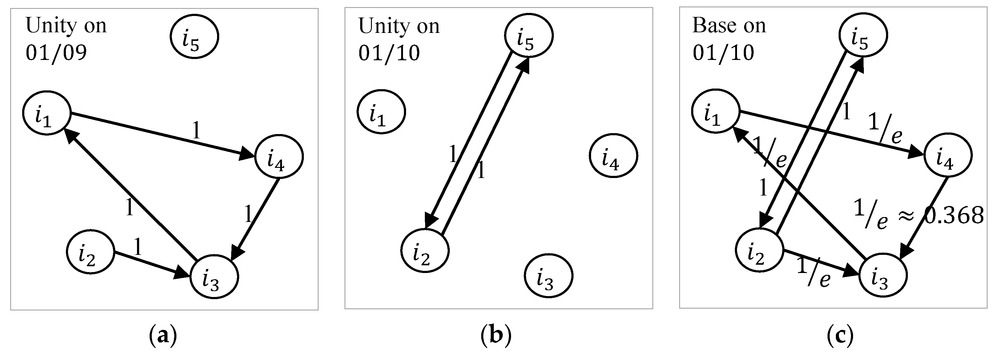
• We construct an item trend graph to sensitively capture the temporal dynamics of item search flow resulting from any external factors.
• We score the user’s preference for item clusters using user-based CF along with methods to overcome the sparsity problem and combine it with the item trend graph.
• We predict the user’s needs with respect to item category and gender based on recent access logs and reflect them in the final recommendation.

Typically, there are two types of recommendation services in online fashion malls. One is top-N recommendation, which suggests N products that are most likely to be preferred from a comprehensive perspective, and another is recommending related items, which are similar to, or possibly more satisfactory than, a given product. Because the former requires a more general approach and is capable of performance evaluation based on historical access data, we focus on a new method for top-N recommendation. Furthermore, considering the commercial purpose of the fashion recommendation service, our goal is to maximize the number of products to be purchased by recommendation, rather than those to be clicked by recommendation.

2. Related Works

To overcome the sparsity problem of using CF, many studies have attempted to increase the accuracy of the similarity between users to improve the recommendation performance. One commonly used approach is a hybrid method [10,11,12] that complements the similarity from the user–item ratings matrix with the similarity of item attributes. However, this method can be applied when the item features are sufficient to explain the item similarity. Instead of using item attributes, some researchers attempted to estimate more accurate similarities [13,14,15] or ratings [16,17] using additional methods or algorithms on the user–item ratings matrix. For example, Gan [13] proposed a method of estimating user similarity by establishing the relationship between user similarity and item similarity as a regression model. Further approaches include a proposal to supplement similarity by the addition of external data [18,19], and to alleviate sparsity through user clustering [20,21]. In this study, we also attempt to reduce sparsity by generating dense ratings from user log data for the most recent months and clustering items based on item similarity.

To generate ratings from implicit feedback datasets, a general approach is to map the users’ activities on items such as click, cart, and purchase into ratings. Nguyen et al. [22] set the proportion of each activity to its score range to generate a personalized score in a functional form; this is not the best scheme using CF based on the common ground ratings. According to [23], using implicit feedback data resulted in a more diverse and accurate recommendation by providing a wealth of unbiased information compared to using explicit ratings.

A major topic in addition to user interest in apparel recommendations is the incorporation of up-to-date fashion trends and seasonality into the recommendations, which requires a model that captures sequential and temporal dynamics from user behaviors. The most popular method for representing such dynamics is a graph, although some studies [24,25,26] suggested models that reflect item sequence without using graphs. Several studies [27,28,29] demonstrated that link analysis methods using Markov chains, such as personalized PageRank [30], can be effectively applied to personalized recommendation considering a sequential pattern based on implicit feedback data. According to [31], exploiting a graph-based model for recommendation makes it easy to not only combine various types of information, but also to represent indirect relationships. Recent research focuses on recommending items with diversity or serendipity, rather than items with only strong relevance or popularity, in order to broaden the user experience and avoid typicality [32,33]. For example, in related entity recommendations for entity queries, diverse but related entities are ranked by link analysis methods on related entity networks based on a co-occurrence relation added by an entity importance vector [33]. Some recommendation systems attempted to reflect both personalization and temporal dynamics by considering user interest as long- and short-term preferences. He and McAuley [34] suggested a sequential prediction model by combining a similarity-based method for long-term preference and a Markov chain for short-term dynamics. For top-N news recommendations, Li et al. [32] utilized long-term user profiles to model users’ general topic interests and short-term profiles to capture the recent preferences with respect to new topics based on user profiling by a time-sensitive weighting scheme. In our proposed framework, we conceptually define the user’s taste as a consistent preference for items and the user’s needs as purchase intent for item categories, which differ conceptually and in terms of object level with the exception of the temporal division of long- and short-term preferences from existing studies.

Finally, the capture of purchase intent of users for item group levels, such as category or brand, requires the analysis of interaction between users and item-groups based on purchase activities over time [35,36]. A recent study regarding purchase prediction for a certain brand [36] identified the most important input feature by comparing purchase prediction performances through various prediction models on action count for three types of activities over several time periods. In contrast to the preference for a brand, the purchase probability of an apparel category is dependent on necessity rather than preference; thus, our study quantifies the purchase intention by modeling whether to buy through daily click counts and cart activities based on the recent few days.

3. Proposed Method

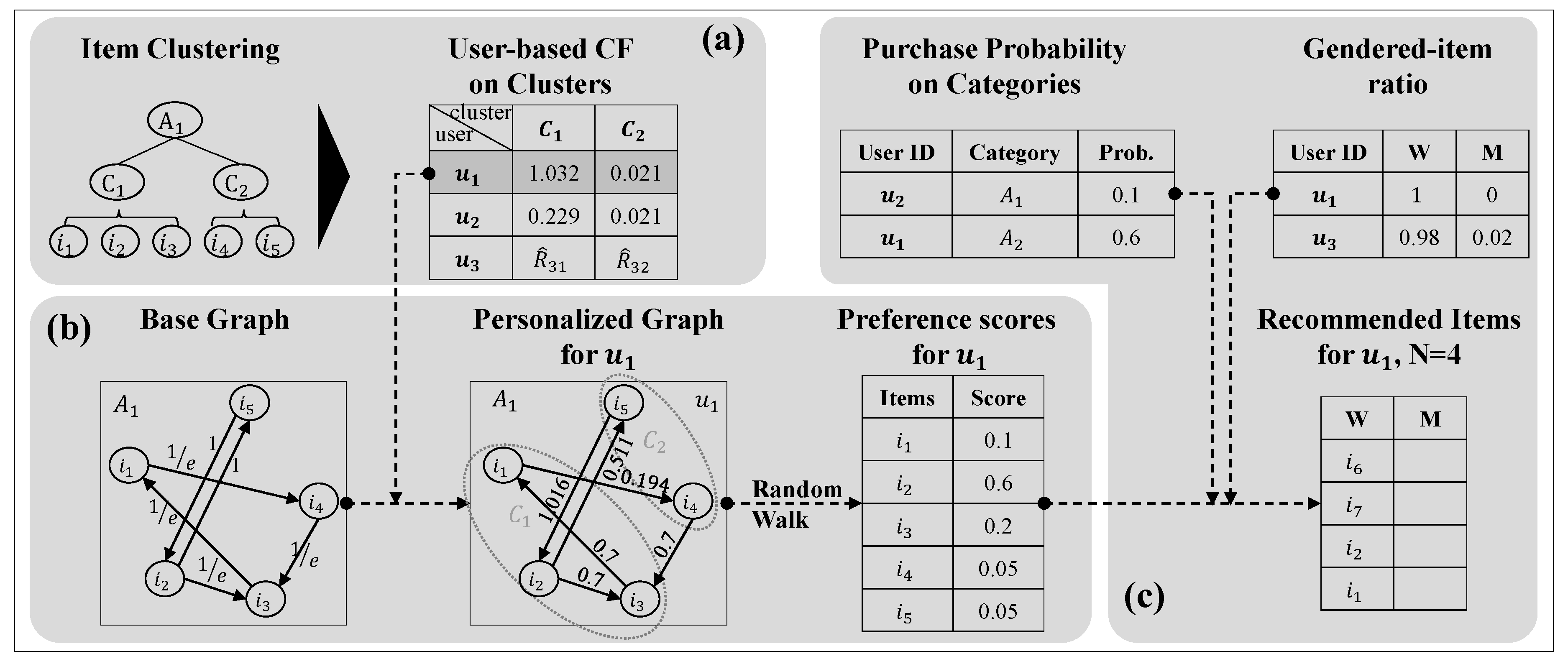
3.1. System Overview

As mentioned earlier, frequent item changes due to fashion trends and seasonality makes data sparsity severe, especially in online apparel shopping. In order to cope with the data sparsity problem, we utilize implicit ratings, i.e., ratings generated from user activity logs. However, the data of implicit ratings are still too sparse to directly apply a CF algorithm. We therefore adopt item clustering based on the implicit ratings, which results in a user–item cluster ratings matrix. Apparel products typically follow the hierarchy of gender–category–item, where the gender takes either female (women’s wear) or male (men’s wear) and the category can be t-shirts, pants, skirts, and so on. The construction of item-clusters implies that we adopt the four-level hierarchy of gender–category–cluster–item, as can be seen in Figure 1. Notice from the figure that items belonging to different categories are not grouped in a same cluster in this study.

Although typical CF algorithms can make personalized recommendations, they are not designed to incorporate temporal dynamics of items. Moreover, we cannot recommend specific items from a CF algorithm based on the user–item cluster rantings matrix. In order to address this problem, we construct directed graphs using the same user activity log and update those as time passes. Frequently visited items by random walks on the graphs would be good candidates for recommendation. This graph-based method, however, does not make personalized recommendations. We therefore combine the user-based CF based on the user–item cluster ratings matrix and the graph-based random walk to incorporate both personalization and temporal dynamics of items, namely fashion trends and seasonality, into an apparel recommender system.

Apparel products are usually selected according to a customer’s needs with respect to categories. For example, a customer needs a t-shirt on one day and a pair of pants on another day. It is also important to know for which product categories the user under recommendation searches. Because apparel products are grouped into women’s and men’s wear, we should consider gender as a key factor for recommendation. It is worth noting that the gender does not refer to a user’s gender and we do not use users’ personal information. We only attempt to determine which category the user searches for between women’s and men’s wear.

Figure 2 represents an overview of our recommendation framework, including all of the abovementioned aspects. After generating implicit ratings from user log data, we perform item-clustering (Figure 2a) and construct a directed base graph (Figure 2b). The user’s preference ratings with regard to item clusters are calculated by a user-based CF algorithm. We construct a personalized graph by projecting the user’s cluster ratings onto the latest item flow graph, and then derive item preference scores through random walks (Figure 2b). Final recommendation items are listed by a combination of item preference scores, the user’s needs for categories, and the gender, as shown in Figure 2c. Each of the stages in our method will be explained in detail as follows: Figure 2a in Section 3.2, Figure 2b in Section 3.3, and Figure 2c in Section 3.4. To aid readers in better understanding our method, we prepared an example dataset in

Table 1. An example of user activity log.

User ID	Item ID	Gender	Category	Activity	Time Stamp
$u_1$	$i_1$	W	$A_1$	CLICK	2017-01-09 20:59
$u_1$	$i_4$	W	$A_1$	CLICK	2017-01-09 21:00
$u_1$	$i_3$	W	$A_1$	CLICK	2017-01-09 21:01
$u_1$	$i_1$	W	$A_1$	CLICK	2017-01-09 21:17
$u_1$	$i_7$	W	$A_2$	CLICK	2017-01-10 19:05
$u_1$	$i_3$	W	$A_1$	ORDER	2017-01-10 19:07
$u_2$	$i_2$	W	$A_1$	CLICK	2017-01-09 11:24
$u_2$	$i_3$	W	$A_1$	CLICK	2017-01-09 11:31
$u_2$	$i_3$	W	$A_1$	CART	2017-01-09 11:36
$u_2$	$i_2$	W	$A_1$	CLICK	2017-01-10 15:27
$u_2$	$i_5$	W	$A_1$	CLICK	2017-01-10 15:31
$u_2$	$i_2$	W	$A_1$	CLICK	2017-01-10 16:02
$u_3$	$i_6$	W	$A_2$	ORDER	2017-01-09 13:37
$u_3$	$i_8$	W	$A_2$	CLICK	2017-01-10 17:18
$u_3$	$i_9$	M	$A_3$	CLICK	2017-01-10 18:09

. This dataset will be used for a stage-by-stage description of our proposed method.

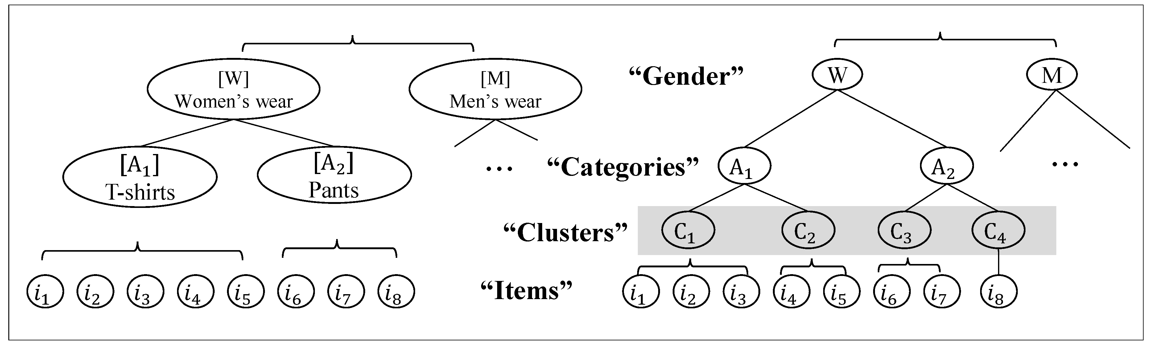
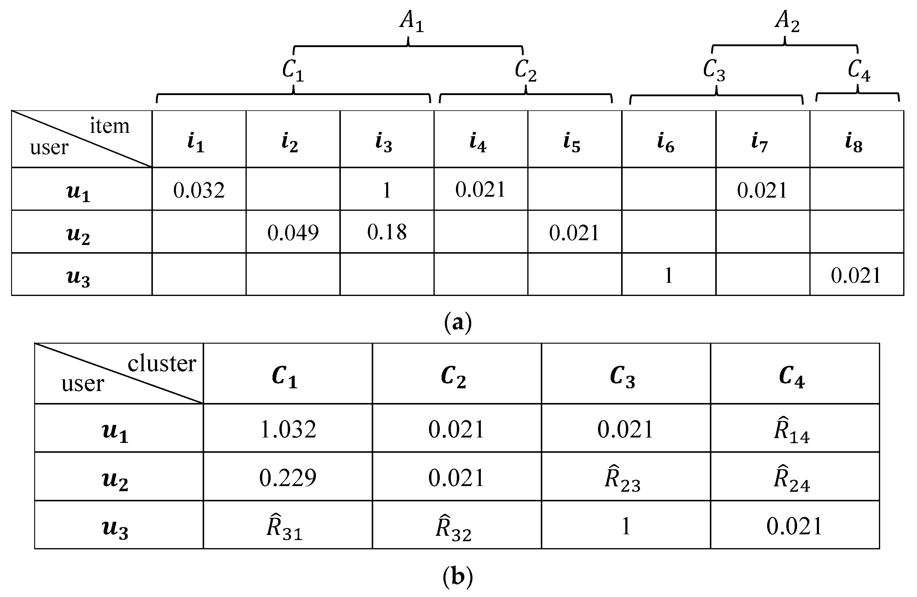
3.2. Rating Item Clusters

Rating the user’s preference for item clusters is performed in three steps: Generating implicit ratings, clustering items, and rating item clusters by CF. We first suggest a weighting scheme that computes an implicit rating by the combination of three types of user activities, i.e., click, cart, and order, from user log data. The click activity implies browsing a webpage of a product and viewing its detailed information. Although the click represents an initial interest in an item, the cart activity shows more interest than the click. A user finally makes a choice by the order activity, which is an even stronger representation of interest in an item. Because these types of activities—click, cart, and order—are applied to almost all types of e-commerce [22,36], we decide to use them in our study in order to preserve the generality of the proposed method. Note that although cart and order are one-time activities, a user can visit the webpage of a specific product multiple times, which means that k clicks can executed by a user. Setting the rating for order activity, $w_{order}$, to the highest value of one (1 if ordered, 0 otherwise), the proportion of cart or click activity to order activity is assigned to its rating, which can be interpreted as the degree of purchase intention when an item is clicked or placed in cart. The rating of cart activity is then computed by

$$w_{cart}=\frac{N\left(CART\cap ORDER\right)}{N\left(CART\right)},$$

(1)

where $N\left(CART\right)$ is the number of cart activities and $N\left(CART\cap ORDER\right)$ is the number of co-occurrences of both cart and order activities in the log data. Accordingly, $N\left(CART\right)-N\left(CART\cap ORDER\right)$ is the number of activities by which a user placed an item in her/his cart but did not purchase it. Owing to the small size, $N\left(CART\right)=1$ and $N\left(CART\cap ORDER\right)=0$ in our example dataset in Table 1. The real dataset used in our experiments shows that approximately 18 percent of cart activities finally resulted in ordering the items in the cart (See Figure 7 in Section 4.3). We now evaluate the click activity, using the fact that more clicks on an item by a user imply her/his stronger interest in it and vice versa. Suppose that a user finally purchased an item after $k$ clicks on it. We count the number of these activities from the log data, which is denoted by $N\left(CLICK\left(k\right)\cap ORDER\right)$. Notice that a user may purchase an item by one click and the user may do so after multiple clicks ($k=1, 2, 3,\cdots$). We then count the number of activities by which a user clicked $k$ times on a certain item, which is denoted by $N\left(CLICK\left(k\right)\right)$. From the example in Table 1, we can obtain $N\left(CLICK\left(1\right)\right)=7$ ($u_1$ clicked $i_3$, $i_4$, and $i_7$ once each, $u_2$ clicked $i_3$ and $i_5$ once each, and $u_3$ clicked $i_8$ and $i_9$ once each), $N\left(CLICK\left(2\right)\right)=1$ ($u_1$ clicked $i_1$ twice), and $N\left(CLICK\left(3\right)\right)=1$ ($u_2$ clicked $i_2$ three times). Because $u_1$ purchased $i_3$ after one click, $N\left(CLICK\left(1\right)\cap ORDER\right)=1$. After finding $N\left(CLICK\left(k\right)\cap ORDER\right)$ and $N\left(CLICK\left(k\right)\right)$ for each $k$ ($k=1, 2, 3,\cdots$), we compute the proportion of purchases to the total number of $k$ clicks:

$$w_{click}\left(k\right)=\frac{N\left(CLICK\left(k\right)\cap ORDER\right)}{N\left(CLICK\left(k\right)\right)}.$$

(2)

Therefore, $w_{click}\left(1\right)=\frac{1}{7}$ from our example, which means that one purchase occurred among seven one-click activities. Instead of using $w_{click}\left(k\right)$ directly, we propose to estimate a function $f$, by fitting $w_{click}\left(k\right)$ on $k$ and use the predicted value $f\left(k\right)={\widehat{w}}_{click}\left(k\right)$, such that the click rating can be generalized and robust to outliers. The $f$ can be any function that can determine the relationship between the number of clicks ($k$) and the proportion of purchases by $k$ clicks ($w_{click}\left(k\right)$), but we believe that a sigmoid function would be a good choice, because a lag phase at small $k$ values and a stabilization phase at large $k$ values tend to appear in purchase behaviors. The example in Table 1 is too small to show a fitted function. See the graph of the function fitted based on our real dataset in Figure 7, where the hollow circles indicate the observed pairs of {$k$, $w_{click}\left(k\right)$} from our real dataset. In summary, $k$ click activity, cart activity, and order activity on a certain item by a user is rated by ${\widehat{w}}_{click}\left(k\right)$, $w_{cart}$, and $w_{order}$, respectively, across all users and all items. Although we applied our rating scheme to three types of activities, notice that Equation (1) can be applied to any other one-time activity and Equation (2) to any other recurring activities if needed.

To finally determine the user $u$’s implicit rating on item $i$ ($r_{ui}$), we first assign ${\widehat{w}}_{click}\left(k\right)$, $w_{cart}$, and $w_{order}$ values based on the user–item–activity combination, and then take the maximum value among those.

Table 2. Generation of ratings by using user activities.

User	Item	Gender	Category	#Clicks	Cart	Order	${\widehat{\mathit{w}}}_{\mathit{c}\mathit{l}\mathit{i}\mathit{c}\mathit{k}}\left(\mathit{k}\right)$	${\mathit{w}}_{\mathit{c}\mathit{a}\mathit{r}\mathit{t}}$	${\mathit{w}}_{\mathit{o}\mathit{r}\mathit{d}\mathit{e}\mathit{r}}$	${\mathit{r}}_{\mathit{u}\mathit{i}}$
$u_1$	$i_1$	W	$A_1$	2			0.032			0.032
$u_1$	$i_3$	W	$A_1$	1		T	0.021		1	1
$u_1$	$i_4$	W	$A_1$	1			0.021			0.021
$u_1$	$i_7$	W	$A_2$	1			0.021			0.021
$u_2$	$i_2$	W	$A_1$	3			0.049			0.049
$u_2$	$i_3$	W	$A_1$	1	T		0.021	0.18		0.18
$u_2$	$i_5$	W	$A_1$	1			0.021			0.021
$u_3$.	$i_6$	W	$A_2$	0		T	0		1	1
$u_3$	$i_8$	W	$A_2$	1			0.021			0.021
$u_3$	$i_9$	M	$A_3$	1			0.021			0.021

shows how the implicit ratings can be generated from the activity ratings by using the example in Table 1. Notice that, owing to the size of the example, we used ${\widehat{w}}_{click}\left(1\right)=0.021$, ${\widehat{w}}_{click}\left(2\right)=0.032$, ${\widehat{w}}_{click}\left(3\right)=0.049$, and $w_{cart}=0.18$, as shown in Figure 7, which were computed from our real dataset.

Based on the user–item ratings matrix, we derive the item similarity of item $i$ and item $j$, $sim\left(i,j\right)$ by calculating the cosine similarity of item vectors as follows:

$$sim\left(i,j\right)=\frac{{\sum }_{u\in \left\{U\left(i\right)\cap U\left(j\right)\right\}}{r}_{ui}·r_{uj}}{\sqrt{{\sum }_{u\in \left\{U\left(i\right)\cap U\left(j\right)\right\}}{r}_{ui}{}^2}·\sqrt{{\sum }_{u\in \left\{U\left(i\right)\cap U\left(j\right)\right\}}{r}_{uj}{}^2}},$$

(3)

where $U\left(i\right)$ and $U\left(j\right)$ denote the set of users who have accessed item $i$ and item $j$, respectively. Then, we cluster items for each category using the affinity propagation (AP) clustering method described in [37]. AP gradually finds exemplars and clustered data points through an iterative message passing procedure, while simultaneously regarding all data points as exemplars. One advantage is that it is not required to specify the number of exemplars in advance. Based on a real-valued similarity matrix, two types of real-valued messages, “responsibility” sent from other data points to candidate exemplars and “availability” sent from candidate exemplars to other data points, are exchanged until the exemplar decisions remain constant for a given number of iterations. Its application to various fields has demonstrated that AP performs clustering with considerably lower errors in less execution time compared to other methods.

After clustering items, we generate user–cluster ratings by summing all $r_{ui}$ within a cluster. If a cluster has $n$ items accessed by user $u$, the rating on the cluster by user $u$ is calculated as $R_{uk}={\sum }_{i=1}^n{r}_{ui}$. Figure 3 represents an example of the generation of a user–cluster ratings matrix based on the example data in Table 2. In this example, we assumed items are clustered as follows: $\left\{i_1,i_2,i_3\right\}\in C_1$, $\left\{i_4,i_5\right\}\in C_2$, $\left\{i_6,i_7\right\}\in C_3$, and $\left\{i_8\right\}\in C_4$.

As can be seen from Figure 3b, some of the cluster preferences are missing if the items in a cluster have not been assessed by the user. The missing preferences are imputed by predicted values via a user-based CF algorithm. In computing user similarities for the user-based CF, we adopt only the numerator, i.e., the inner product, from the original cosine similarity to reflect the difference in ratings. This represents the relative importance of each activity. Thus, the similarity between user $u$ and $v$, $sim\left(u,v\right)$, is computed as follows:

$$sim\left(u,v\right)={\displaystyle \sum }_{i\in \left\{I\left(u\right)\cap I\left(v\right)\right\}}{R}_{ui}·R_{vi},$$

(4)

where $I\left(u\right)$ is a set of clusters accessed by user $u$. For example, $sim\left(u_1,u_2\right)=\left(1.032\right)·\left(0.229\right)+\left(0.021\right)·\left(0.021\right)\cong 0.237$ in Figure 3b. Then, the predicted rating on cluster $k$ by user $u$, ${\widehat{R}}_{uk}$ is computed as follows:

$$sim\left(u,v\right)={\displaystyle \sum }_{i\in \left\{I\left(u\right)\cap I\left(v\right)\right\}}{R}_{ui}·R_{vi},$$

(5)

where $U$ is the set of all users. Here, we do not subtract the user’s mean rating from each rating, whereas the original user-based CF does, because the cluster preference $R_{uk}$ does not contain bias, unlike explicit ratings by users. Notice from Figure 3a that owing to data sparsity, ${\widehat{r}}_{34}$ and ${\widehat{r}}_{35}$ cannot be computed by user-based CF, because $sim\left(u_3,u_1\right)=sim\left(u_3,u_2\right)=0$. After clustering items, ${\widehat{R}}_{32}$ can be calculated, because $sim\left(u_3,u_1\right)\ne 0$, as can be seen from Figure 3b. In this way, we cope with the data sparsity problem through item clustering, computing more user similarities based on item clusters, and imputing missing preferences. The cluster preferences, ${\widehat{R}}_{uk}$ and $R_{uk}$, are used to construct personalized graphs in the subsequent stage of our recommendation framework.

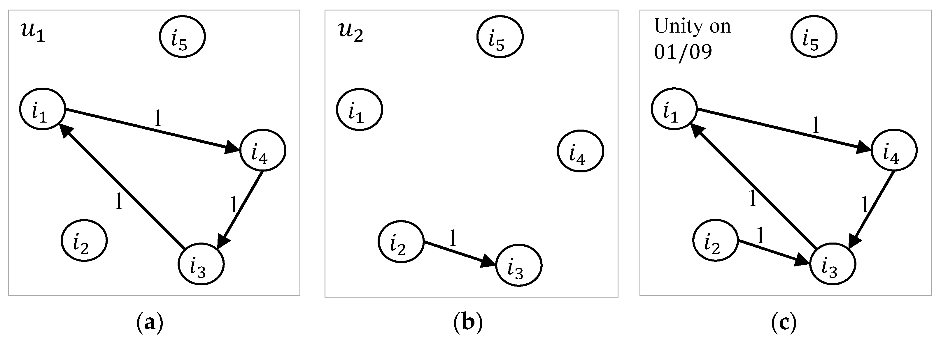
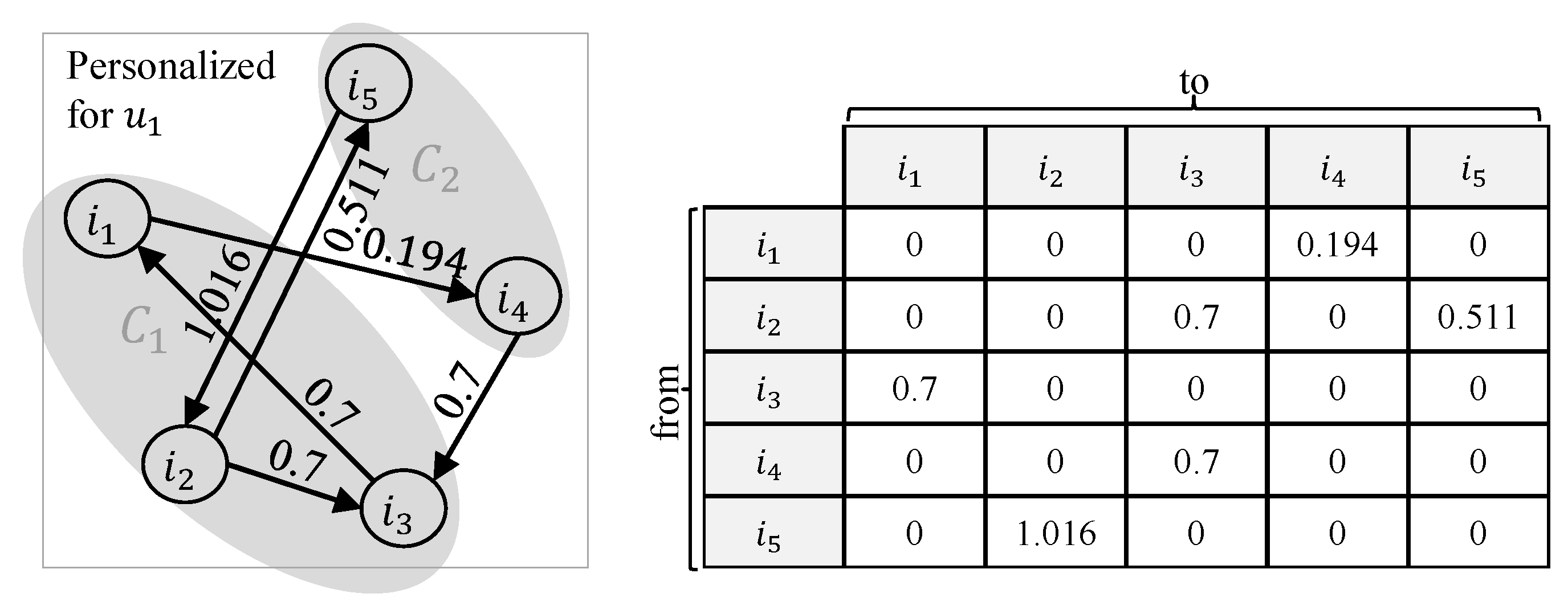
3.3. Personalized Random Walk

In this subsection, we describe the stage for scoring item preferences, which consists of three steps: Generating a base graph, personalizing the graph, and scoring item preferences through random walks. We begin with constructing a directed graph with items as nodes and the number of transitions as edge weights; this is called a unity graph. From the sequential click data in Table 1, the transitions by $u_1$ for $A_1$ on 9 January 2017 are expressed as $\left(i_1,i_4\right)$, $\left(i_4,i_3\right)$, and $\left(i_3,i_1\right)$ in the form of (source node, target node). Figure 4a,b depicts the directed graphs for $u_1$ and $u_2$, respectively. In succession, the integration of the two graphs by summing edge weights on the same transition results in the unity graph shown in Figure 4c. Here, we define a unity graph from the entire click data generated for one day, which represents the item click flow of the day.

The base graph is created by sequentially integrating the unity graphs such that the graph represents the trend of the latest item selection. We initially set the oldest unity graph as a base graph and repeatedly update the base graph on a daily basis, using a temporal weighting scheme. Let $w_{old}\left(x,y\right)$ be an edge weight from node $x$ to node $y$ in the latest base graph, which was updated yesterday, and $w_0\left(x,y\right)$ be an edge weight in a unity graph of today, which is not yet reflected in the base graph. Then, the edge weight in the updated base graph, $w_{new}\left(x,y\right)$, is calculated as follows:

$$w_{new}\left(x,y\right)=\max \{\tau ·w_{old}\left(x,y\right), w_0\left(x,y\right)\}, 0<\tau <1.$$

(6)

By setting a unity graph on 9 January 2017 in Figure 4c as an initial base graph and applying $\tau =1/e$, an updated base graph on 10 January 2017 is created as shown in Figure 5. Notice that the new edge weight from $i_1$ to $i_4$ on the updated base graph on 10 January 2017 is $w_{new}\left(i_1,i_4\right)=\max \left\{\raisebox{1ex}{$1$}\!\left/ \!\raisebox{-1ex}{$e$}\right.,0\right\}=\raisebox{1ex}{$1$}\!\left/ \!\raisebox{-1ex}{$e$}\right.$.

In Equation (6), any change in the new edge weight is sensitively reflected in the new base data by decreasing the previous edge weight. In addition, we take the maximum of the two weights instead of the sum to provide items with different sales periods with a fair standard by reflecting the click data for one day for each weight. Therefore, the base graph represents not only the latest item popularity, but also the rich connectivity for long-tail items. For reference, the recommendation of related items for a given item is easily derived in this step by sorting the target nodes of outgoing edges from a given node according to their edge weights.

In the next step, a personalized graph is created by combining the user’s preferences on clusters, $R_{uk}$, with the edge weight on the base graph, $w_{new}\left(x,y\right)$. Let $C_k$ be an item set contained in cluster $k$. Then, a personalized edge weight from $x$ to $y\in C_k$ for user $u$, $w_u\left(x,y\right)$ is defined as follows:

$$w_u\left(x,y\right)=\left(1-{\alpha }_1\right)·w_{new}\left(x,y\right)+{\alpha }_1·R_{uk}, y\in C_k and 0<{\alpha }_1<1.$$

(7)

Figure 6a illustrates a personalized graph in $A_1$ for $u_1$. It was created from the base graph in Figure 5c. The preferences of $u_1$ on $C_1$ and $C_2$ are $R_{11}=1.032$ and $R_{12}=0.021$, respectively, and ${\alpha }_1=0.5$ was chosen in this example. Therefore, the edge weight from $i_5$ to $i_2\in C_1$ becomes $w_1\left(i_5,i_2\right)=\left(1-0.5\right)\times 1+0.5\times 1.032=1.016$ and that from $i_2$ to $i_5\in C_1$ is updated to $w_1\left(i_2,i_5\right)=\left(1-0.5\right)\times 1+0.5\times 0.021=0.511$.

Note that $R_{uk}$ (or ${\widehat{R}}_{uk}$) is applied to an incoming node, $y\in C_k$ in Equation (7), to control the item selection flow to the items in cluster $k$. In addition, Equation (7) adjusts the proportion of common trends and personal taste using ${\alpha }_1$, which practically serves to filter out the latest and commonly popular items from the personally preferred items within a cluster. The personalized edge weights are then used to construct the adjacency matrix in Figure 6b. We divide each row of the adjacency matrix by the row sum to convert it into a transition matrix used for a Markov chain. Performing $n$ random walks on the Markov chain derives the item preferences by simulating the user’s selection process with defined transition probabilities. The preference score for item $i$ by user $u$, ${\widehat{r}}_{ui}$, can finally be calculated as follows:

$${\widehat{r}}_{ui}=\frac{n\left(i\right)}{n},$$

(8)

where $n\left(i\right)$ is the number of visits on node $i$ through $n$ random walks.

3.4. Reflecting User’s Needs

We mentioned previously that it is important to determine which category and item-gender the user under recommendation needs. Based on user’s preferences in the previous stage, we generate a final list for recommendation by additionally reflecting user’s purchase intention on certain categories and the long-term interest for item-gender.

Some users shop according to their purchase needs in certain categories, which leaves access logs of items in corresponding categories. Therefore, our strategy is to adjust the preference score according to the category purchase probability to improve the recommendation quality. To build a prediction model for category purchase probability from logs with three types of activities, we extract the number of daily clicks and carts for $T$days prior to when any purchase activity occurred, which act as predictors, and the purchase or nonpurchase of the category at the time as a dependent variable. In setting the dependent variable, whether a category is purchased or not as a binary number for a classifier yields the purchase probability of the category. Formally, let $v_{kt}$ and $w_{kt}$ be the daily frequencies for clicks and carts, respectively, for category $k$ that occurred $t$ days $(t\in \left\{0,1,\dots ,T\right\}$) prior to the purchase time, where $t=0$ implies the purchase day. Then, the purchase probability for category $k$, $p_k$, is expressed as follows:

$$p_k=f\left(v_{k0},w_{k0},v_{k1},w_{k1},\cdots ,v_{kT},w_{kT}\right), k=1,2,\dots ,n.$$

(9)

For example, by setting $T=1$, the training data are constructed from the log in Table 1, as shown in

Table 3. Preparation of training data from user log in Table 1.

User	Category	${\mathit{v}}_{10}$	${\mathit{w}}_{10}$	${\mathit{v}}_{11}$	${\mathit{w}}_{11}$	Order
$u_1$	$A_1$	0	0	4	0	1
$u_1$	$A_2$	1	0	0	0	0
$u_3$	$A_2$	0	0	0	0	1

. Notice that $u_2$ did not order any item and $u_3$ does not have any click and cart log for $t=1$ (8 January 2017) and $t=0$ (9 January 2017, the date when $u_3$ ordered $i_6$) in our limited example. The former results in the activity log of $u_2$ not making a training example, and the latter results in the training example of ($v_{10}=0,w_{10}=0,v_{11}=0,w_{11}=0, order=1)$.

In Equation (9), $f$ can be any classifier such as binary logistic regression, a random forest, or a neural network. Now, the probability that user $u$ will purchase items in category $k$, ${\widehat{p}}_{uk}$, is predicted by inputting $\left\{v_{k0},w_{k0},v_{k1},w_{k1},\cdots ,v_{kT},w_{kT}\right\}$ by user $u$ to the trained classifier. That is, the purchase probability of $u_2$ for $A_1$ on 10 January 2017 in our example is ${\widehat{p}}_{21}=f\left(3,0,2,1\right)$. With the predicted probability ${\widehat{p}}_{uk}$, the final item preference score for item $i$ contained in category $k$ by user $u$, ${\widehat{s}}_{ui}$, is calculated as follows:

$${\widehat{s}}_{ui}=\left(1-{\alpha }_2\right){\widehat{r}}_{ui}+{\alpha }_2{\widehat{p}}_{uk},0<{\alpha }_2<1.$$

(10)

Because the classification model $f$ is trained from the user log for $T$ recent days, if user $u$ has no access log for category $k$ during that time period, then ${\widehat{p}}_{uk}=0$. Therefore, we employ a weighted average scheme to combine item preference and purchase intention of category, instead of a multiplication-based combination method, such as the geometric mean, as applied in previous studies [14,35]. It is also convenient to adjust the weight of each component by controlling the value of ${\alpha }_2$.

It is known that not all but most users access either women’s or men’s wear. Therefore, it is necessary to determine the user’s interest on item-gender to minimize the loss of sales opportunity due to unnecessary item exposure. However, we would rather suggest listing both women’s and men’s wear than display either one set or the other, because it is still possible that the user would like to view the items of different gender. To utilize these, we adjust the proportion of women’s and men’s wear in our top-$N$ recommended items. We attempt to obtain the long-term interest for gendered items by summing the implicit ratings ($r_{ui}$) for accessed items by gender. Let $S_{uW}$ and $S_{uM}$ denote the total ratings by user $u$ for women’s and men’s wear, respectively. Then, the ratio and the number of women’s items to be recommended to user $u$, ${\rho }_{uW}$ and $N_{uW}$, can be expressed as follows:

$${\rho }_{uW}=\frac{S_{uW}}{S_{uW}+S_{uM}},$$

(11)

$$N_{uW}=Round\left(N·{\rho }_{uW}\right),$$

(12)

where $Round\left(x\right)$ represents the nearest integer to $x$, and $N$ is the total number of recommended items. From Equation (12), we allocate $N_{uW}$ items for women’s wear and $\left(N-N_{uW}\right)$ items for men’s wear. In the case of $u_3$ in Table 2, ${\rho }_{3W}=1.021/\left(1.021+0.021\right)\cong 0.98.$ We therefore recommend 29 women’s items and 1 men’s item to user $u_3$ if a total of 30 items are recommended to the user ($N=30$).

4. Numerical Experiments

4.1. Real World Dataset

To evaluate our proposed recommendation framework for online apparel shopping, we use online users’ access log data from 1 December 2016 to 10 March 2017 from a commercial apparel company in South Korea. We selected 12 categories, 7 for female and 5 for male, by removing categories such as accessories and suits, which have considerably different preference patterns from casual clothes. According to our research goal, we measure the performance of top-$N$ recommendation based on the items purchased by the users. Of these data, we employ the data for the first three months, from 1 December to 28 February as training data, and the purchase data for the last 10 days, from 1 March to 10 March as test data. To rigorously assess the performance of the recommender system, some of the test data are removed, including (1) data of users and items that had no history in the training data and (2) data of the purchased items that had access history by the test user in the training data because a user generally leaves multiple clicks or cart logs for an item just before purchasing it. This access history is assigned a high rating by our rating scheme, which leads to a high ranking in the recommendation list. Therefore, we do not count it as a recommendation success in the evaluation, although this decreases the accuracy of the recommendation. As a result, we used a total of 26,721,693 access logs by 1,844,683 users, resulting in 18,979 items for training data and 1961 purchased items by 1164 users for test data. Of the total access logs, 93%, 5%, and 2% are click, cart, and order activity, respectively. The user–item ratings matrix, of which the size is 1,844,683-by-18,979, has 70,020,477 ratings. It means that the sparsity of the ratings matrix is 99.8%. Of the 1,844,683 users, about 20% has contacted both women’s and men’s items in training period, and about 30% provided their gender information. It is worth noting that the gender information is quite limited and inefficient to explain the preference on gendered items. The 18,979 items consist of 53% women’s and 47% men’s wear.

4.2. Performance Measurement

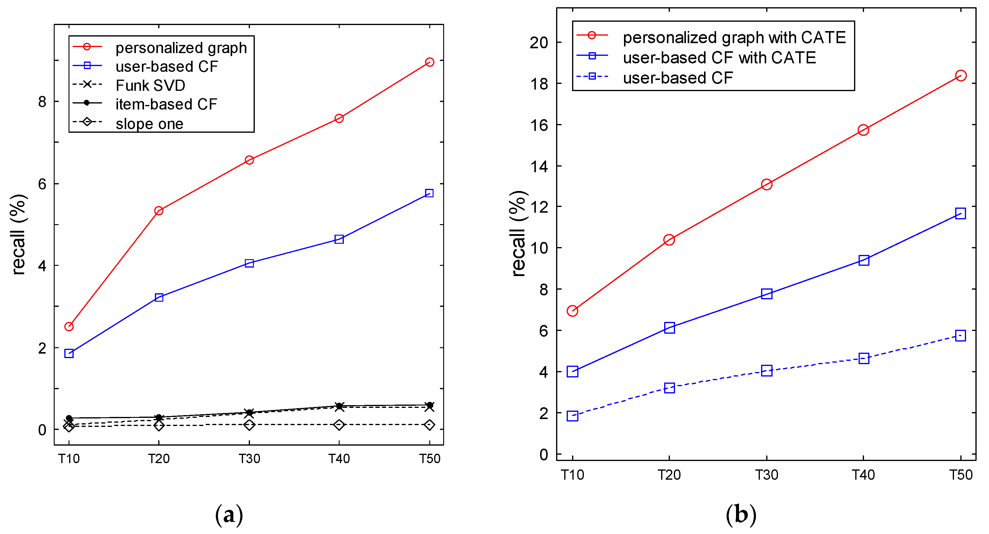
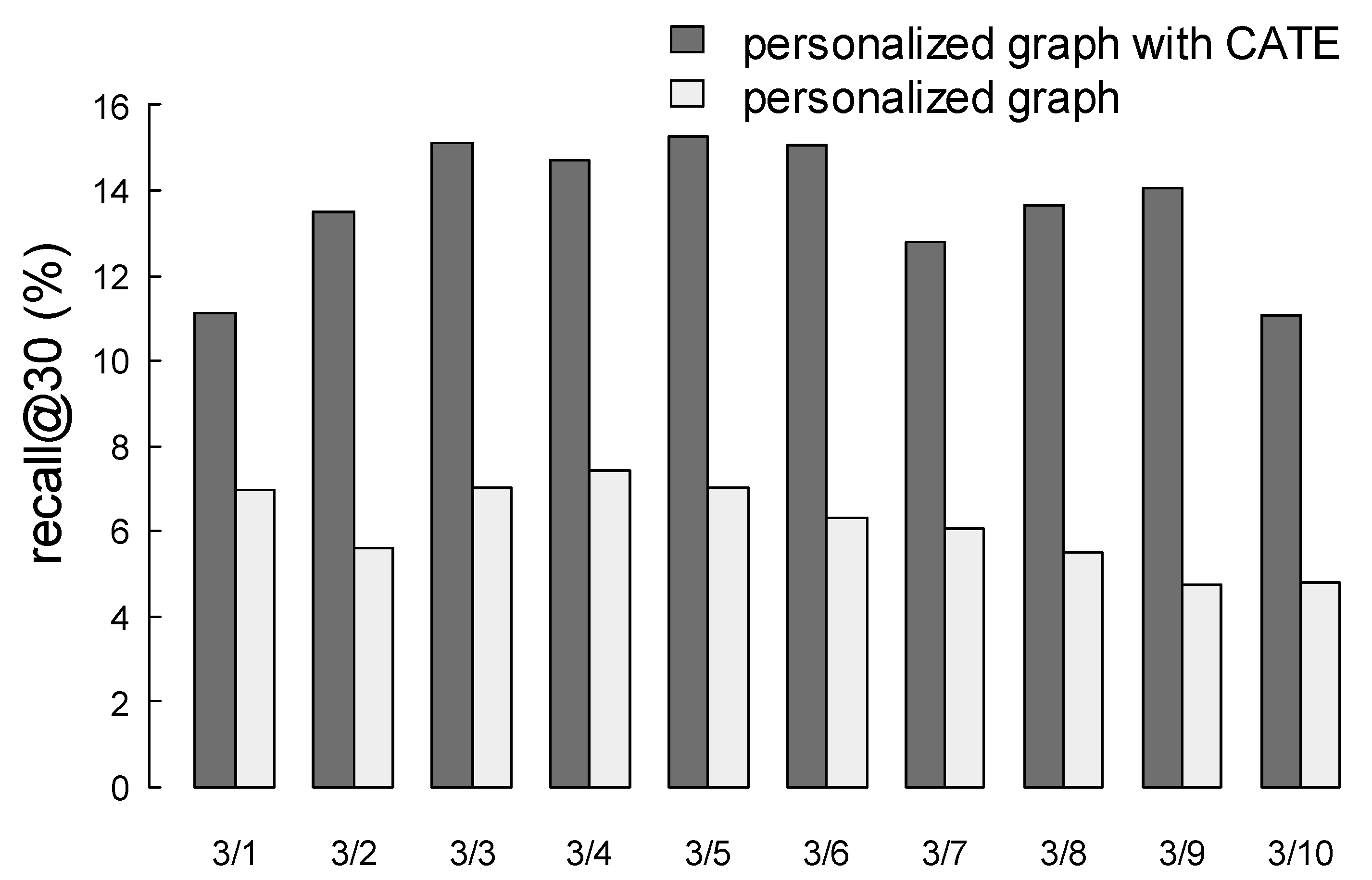
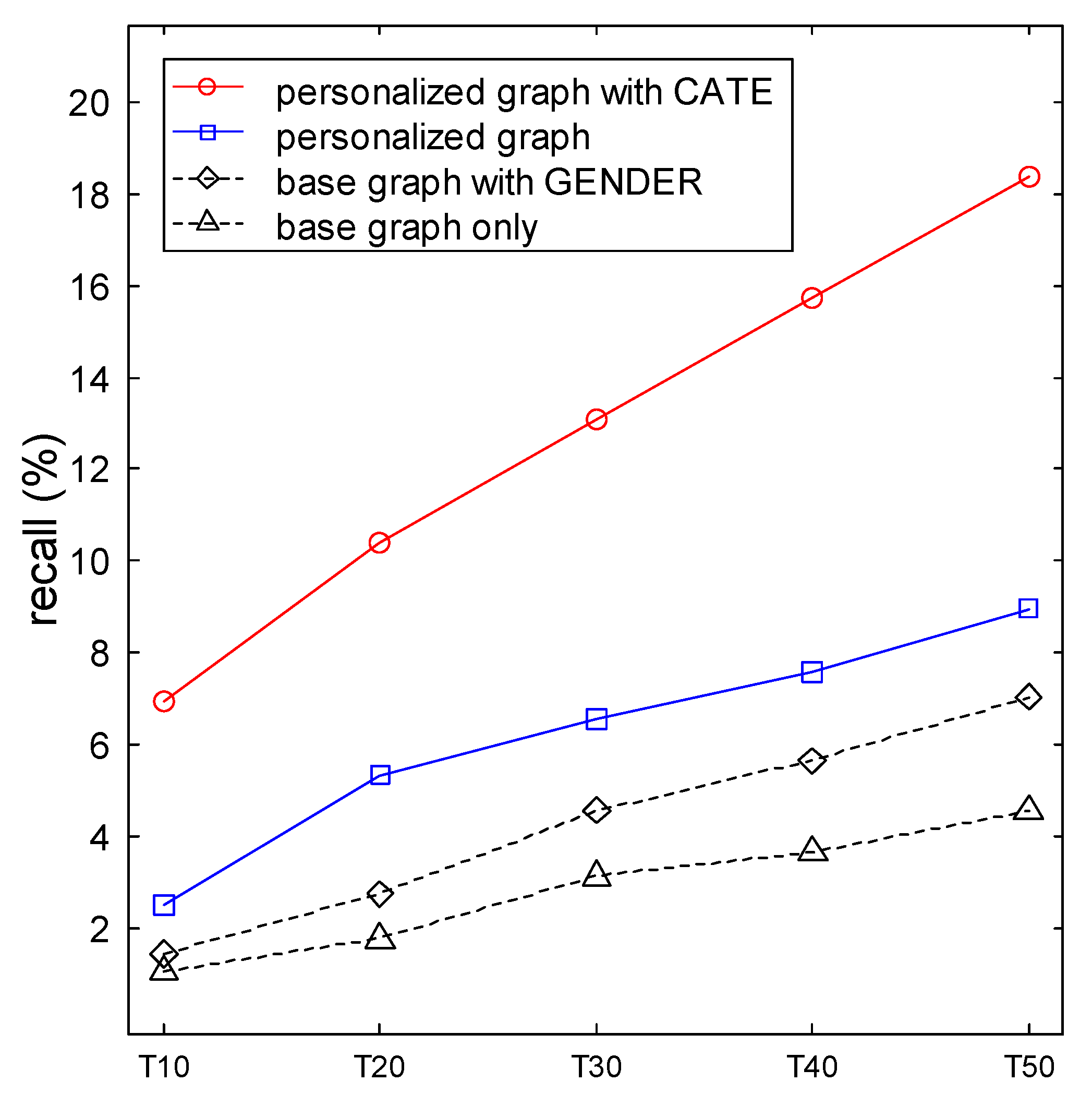
To measure the performance for our proposed recommender system based on purchase data, we adopt the recall (hit rate: True positive rate) instead of the precision because: (1) The number of purchased items is extremely small and practically limited compared to the total number of items presented, and therefore it is inevitable that a large portion of recommended items are not purchased; (2) the exact false positive is difficult to measure from the historical purchase data, because it is possible that purchased items are different if the recommended items are actually presented to users. Consider that the dataset described in Section 4.1 is a purchase history of users without any recommender systems. It means that the data is not a result from recommendation. For the purpose of performance comparison, we therefore count the number of items purchased based on the assumption that top-$N$ recommended items were presented to users [23,38,39,40]. At each $N$, the recall by a user is computed as follows:

$$recall@N=\frac{number of purchased items among N recommended items}{total number of items purchased}.$$

(13)

We varied the value of $N$ from 10 to 50 in increments of 10 and analyzed how the recall would change with several methods and parameters.

4.3. Results

Regarding the experimental results, it is noted that the purchase of apparel items differs from the purchase or consumption of digital content such as movies and news in terms of item price and access patterns. According to our experimental data, the 10% truncated mean of the prices of 18,979 items is 167,529 KRW (approximately 147.6 USD), and 70% of all users who purchased any items for one month purchased only one or two items. Even for 90% of users, fewer than five items were bought. This implies that in most cases, we should select $N$ items containing one or two items out of the total of 18,979 items to make a successful recommendation. Under the assumption that a user purchased only one item during the test period (1 March to 3 March), if we randomly recommend 30 items to the user, the expected recall of the random recommendation is $\frac{\left(\begin{array}{c}n-1\\ N-1\end{array}\right)}{\left(\begin{array}{c}n\\ N\end{array}\right)}=\frac{\left(\begin{array}{c}18978\\ 29\end{array}\right)}{\left(\begin{array}{c}18979\\ 30\end{array}\right)}\cong 0.158\%$, where $n$ is the total number of items and $N$ is the number of recommended items. Likewise, for a user who purchased only two items during the test period, the expected recall becomes $\frac{\left(\begin{array}{c}n-2\\ N-2\end{array}\right)}{\left(\begin{array}{c}n\\ N\end{array}\right)}·1+\frac{2·\left(\begin{array}{c}n-2\\ N-1\end{array}\right)}{\left(\begin{array}{c}n\\ N\end{array}\right)}·\frac{1}{2}\cong 0.158\%$. In addition, a relatively high item price encourages users to make a careful and conservative decision, owing to limited resources. This implies that for multiple items with high preference, they continue comparisons to find the best one or two items instead of easily effecting extra expenditure. In general, the recall in apparel recommendation is not as high as that in other domains, and it is not easy to improve.

Using the rating scheme in Section 3.2, we determined the values of $w_{cart}$ and $w_{click}\left(k\right)$ based on our real dataset and then fitted a function of purchase rate ($f$) to the number of clicks to obtain ${\widehat{w}}_{click}\left(k\right)$ values. A sigmoid function was employed in our experiments, as shown in Figure 7. Examples of ${\widehat{w}}_{click}\left(k\right)$ are ${\widehat{w}}_{click}\left(2\right)=0.032$ and ${\widehat{w}}_{click}\left(10\right)=0.232$.

In our proposed framework, we determine three parameters, namely $\tau$ in Equation (6), ${\alpha }_1$ in Equation (7), and ${\alpha }_2$ in Equation (10), which are not trivial owing to the mutual effects among parameters and the limitation of calculation resources. Therefore, for efficient parameter tuning, we first identified the best parameter settings through 440 test users for one day, and then confirmed their effectiveness through 1164 test users for the remaining days. A decay factor, $\tau$, required to generate a base graph indicates how strongly past connectivity is reflected, and the reflection of current click flow decreases relatively for a smaller $\tau$. Under a fixed ${\alpha }_1$, a reflection rate of user preference on a base graph, we obtained the best result with $\tau =1/e$ by comparing recall values at $\tau =1/\sqrt{2}, 1/e, 1/5$. We then confirmed ${\alpha }_1=0.5$ by several experiments according to various ${\alpha }_1$ values under a fixed $\tau =1/e$. Because the reflection rate of category purchase probability, ${\alpha }_2$, affects the optimal ${\alpha }_1$, we determined the best combination of ${\alpha }_1$ and ${\alpha }_2$, which is given by ${\alpha }_1=0.3$ and ${\alpha }_2=0.6$.

Based on the determined parameters, we measured the effect of the proposed methods separately by comparing the results of the applied case with the nonapplied case based on 1164 users. We first measured the effect of gendered-item interest (GENDER), cluster preferences (personalized graph), and category purchase probability (CATE), respectively, on a base graph with no personal taste by comparing four cases: (1) Base graph only, (2) base graph with GENDER, (3) personalized graph, and (4) personalized graph with CATE. As a result, the three effects were proven to considerably improve the recommendation performance, as depicted in Figure 8. In addition, Figure 8 shows that the reflection of category purchase probability remarkably improved the recommendation accuracy, in which the recall was more than doubled.

To validate the effectiveness of the whole framework, we compared our final performance with that of four other prevailing methods: (1) User-based CF on user–item ratings matrix, (2) item-based CF on user–item ratings matrix, (3) slope one, which is the weighted slope one in [41], and (4) funk SVD, which is the regularized singular value decomposition for CF in [42]. Notice that, based on the implicit ratings ($r_{ui}$) in Section 3.2, we can employ the four abovementioned methods to make recommendations. In Figure 9a, the comparison of the recall values from the four existing methods with that from the proposed method (personalized graph) demonstrates that our proposed method significantly outperformed the existing methods. Because the item-based CF, slope one, and funk SVD methods clearly performed the worst, we excluded these methods from our further comparative experiments. From Figure 8, we found that incorporating the category purchase probability into the recommendation could improve the performance. We, therefore, applied the category purchase probability to the predicted ratings from the user-based CF and the proposed personalized graph using ${\alpha }_2=0.9$. The former is denoted by “user-based CF with CATE” and the latter is denoted by “personalized graph with CATE.” As can be seen from Figure 9b, our proposed method (personalized graph with CATE) performed the best. Nevertheless, the reflection of the category purchase probability on the user-based CF resulted in a substantial improvement, as in our method.

5. Discussion

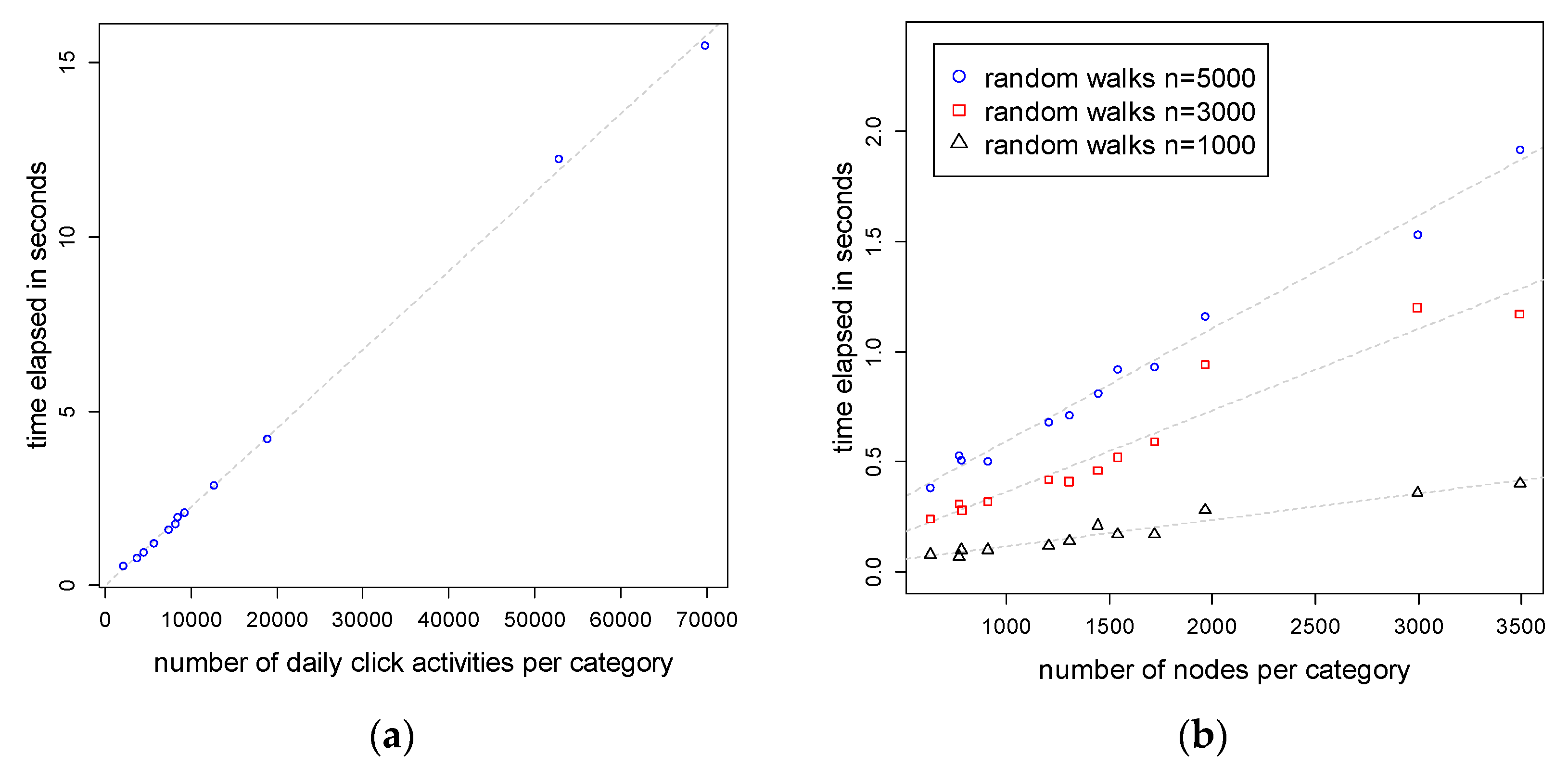
5.1. Computational Complexity

In our proposed method, two major computations are required for its implementation: (1) Initial creation and daily update of a base graph and (2) random walks on the graph. A unity graph is generated by summing the sequential click activities by users for a day, and a base graph is generated by combining $T$ unity graphs, where $T$ is the number of days that we consider to update the graph. Therefore, the computational complexity of generating a unity graph is $O\left(c\right)$, and that of generating a base graph is $O\left(Tc\right)$, where $c$ is the number of click activities for a day. Figure 10a shows the time elapsed to generate unity graphs for 12 categories with different numbers of click activities. We can observe that the computational time linearly increases as the number of clicks increases, and approximately 15 s were spent for more than 70,000 clicks. The computational time for random walks is proportional to the number of nodes on the graph (n), and the number of random walks ($N$), which results in $O\left(Nn\right)$. As illustrated in Figure 10b, the elapsed time linearly increases with respect to the number of nodes and the number of random walks. Our experiments show that 5000 random walks on 3500 nodes took only approximately 20 s. This empirical study on computational time proves that our proposed method is tangible and useful in practice. These experiments were performed on a computer with an Intel i5 processor running at 2.60 GHz using 8 GB of RAM, on x64 Windows 7.

It would be worthwhile to compare the computational complexity of the proposed method with those of existing methods. For a fair comparison, let $m$ be the number of users and $n$ be the number of items. The complexity of training part of our method is $O\left(nm\right)$, which is the same with that of the user-based CF under the reasonable assumption that $Tc\ll nm$. The prediction part becomes $O\left(Nn\right)$ as explained above.

Table 4. Computational complexities.

Method	Training	Prediction
Proposed	$O\left(mn\right)$	$O\left(Nn\right)$
User-based	-	$O\left(mn\right)$
Item-based	$O\left(m{n}^2\right)$	$O\left(n\right)$
Slope one	$O\left(m{n}^2\right)$	$O\left(n\right)$
Funk SVD	$O\left(mnk\right)$	$O\left(1\right)$

compares the computational complexities of the methods tested in our experiments, where the complexities of existing methods came from [43]. For the Funk SVD, $k$ is the number of latent features.

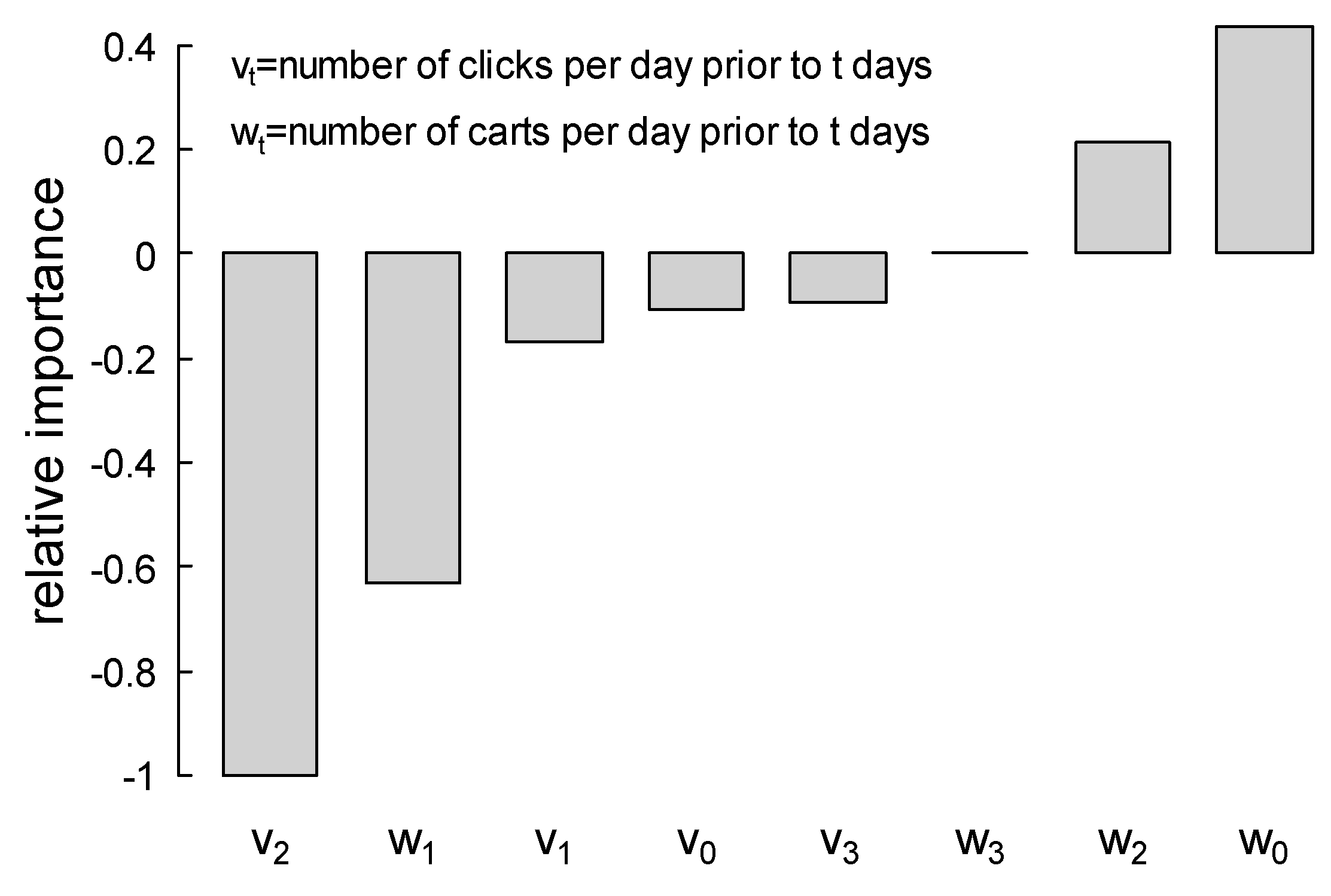
5.2. Analysis on Purchase Intention for Categories

To train a classifier for predicting the category purchase probability, we used clicks and cart data for four days, $T=3$ in Equation (9), $\left\{v_{k0},w_{k0},v_{k1},w_{k1},v_{k2},w_{k2},v_{k3},w_{k3}\right\}$ for category $k$. We adopted a single-hidden-layer neural network and tested various numbers of hidden nodes ranging from 2 to 20. A neural network classifier with 15 hidden nodes (8-15-2 structure) showed a better result with mean absolute error $\left(MAE\right)=0.16$ than with the other two classifiers: Logistic regression with $MAE=0.19$ and random forest with $MAE=0.17$. The relative importance of variables for the neural network model is shown in Figure 11, which indicates that clicks two days prior and carts on the current day for a category have the strongest negative and positive relationships, respectively, with the purchase probability. In addition, we observe that clicks and carts three days prior do not have a significant effect on the purchase probability.

Because we derived the base graph and user preference for the personalized graph using training data until 28 February and evaluated our model using the test data from 1 March, a gradual degradation in performance inevitably occurs according to the dates of the test data. We observed a daily temporal trend of the recall values at $N=30$ from 1 March to 10 March in two cases: (1) Personalized graph with CATE and (2) personalized graph. In Figure 12, although the recall in case (2) exhibits a gradual decrease since 6 March, that in case (1) has no distinct degradation; it is presumed that using data for the most recent three days for CATE complemented the recentness for training data that is no longer valid. Therefore, the application of CATE with low computational complexity for real-time services contributes to not only improving performance, but also to reducing the calculation cost by extending the length of the calculation cycle of the user preferences.

6. Conclusions

In this paper, we demonstrated that our proposed recommender framework contributes to effectively and systematically improving the recommendation accuracy for apparel items by integrating user preferences and needs into the latest item trend. The generation of the user–item ratings matrix by the suggested rating scheme alleviated the data sparsity problem and increased the effectiveness of the algorithms. The user-based CF on cluster preferences increased the diversity of the recommended items and the reflection of these ratings onto the base graph served a combination of personal taste and common trends. In addition, integrating the item preference with category purchase intention remarkably improved the performance of the recommendation.

An additional advantage of the proposed system is that the separated module structure enables the optional use of modules and the selective operation of the reflection parameters, which allows the adjustment of the calculation cost. The optional extension to other domains is a possible aspect to be addressed in future work. A further topic is the personalization of the reflection rate to optimally balance the taste and trend by analysis of the difference in ranking between recommended and purchased items.

References

1. Statista. Share of Internet Users Who Have Ever Purchased Products Online as of NOVEMBER 2016, by Category. Available online: http://www.statista.com/statistics/276846 (accessed on 1 November 2017).
2. Goto, M.; Mikawa, K.; Hirasawa, S.; Kobayashi, M.; Suko, T.; Horii, S. A new latent class model for analysis of purchasing and browsing histories on EC sites. Ind. Eng. Manag. Syst. 2015, 14, 335–346. [Google Scholar] [CrossRef]
3. Golubtsov, N.; Galper, D.; Filchenkov, A. Active adaptation of expert-based suggestions in ladieswear recommender system LookBooksClub via reinforcement learning. In 1st International Early Research Career Enhancement School on Biologically Inspired Cognitive Architectures, FIERCES on BICA 2016; Klimov, V.V., Rybina, G.V., Samsonovich, A.V., Eds.; Springer Verlag: Berlin, Germany, 2016; Volume 449, pp. 61–69. [Google Scholar]
4. Perkinian, C.; Vikkraman, P. An intelligent apparel recommendation system for online shopping using style classification. Int. J. Appl. Bus. Econ. Res. 2015, 13, 671–686. [Google Scholar]
5. Wakita, Y.; Oku, K.; Huang, H.H.; Kawagoe, K. A Fashion-Brand Recommender System Using Brand Association Rules and Features. In Proceedings of the 4th IIAI International Congress on Advanced Applied Informatics (IIAI-AAI), Okayama, Japan, 12–16 July 2015; pp. 719–720. [Google Scholar]
6. Chen, K.T.; Luo, J. When Fashion Meets Big Data: Discriminative Mining of Best Selling Clothing Features. In Proceedings of the 26th International World Wide Web Conference 2017, WWW 2017 Companion, Perth, Australia, 3–7 April 2017; pp. 15–22. [Google Scholar]
7. Guan, C.; Qin, S.; Ling, W.; Ding, G. Apparel recommendation system evolution: An empirical review. Int. J. Cloth. Sci. Technol. 2016, 28, 854–879. [Google Scholar] [CrossRef]
8. Jagadeesh, V.; Piramuthu, R.; Bhardwaj, A.; Di, W.; Sundaresan, N. Large scale visual recommendations from street fashion images. In Proceedings of the 20th ACM SIGKDD International Conference on Knowledge Discovery and Data Mining (KDD), New York, NY, USA, 8 January 2014; pp. 1925–1934. [Google Scholar]
9. Yu, L.; Dong, A. Hybrid product recommender system for apparel retailing customers. In Proceedings of the 2010 WASE International Conference on Information Engineering (ICIE), Beidaihe, Hebei, China, 14–15 August 2010; pp. 356–360. [Google Scholar]
10. Mu, W.; Meng, F.; Chu, D. A Collaborative Filtering Recommendation Algorithm Based on User Preferences on Service Properties. In Proceedings of the International Conference on Service Sciences (ICSS), Wuxi, China, 22–23 May 2014; pp. 43–46. [Google Scholar]
11. Sengottuvelan, P.; Gopalakrishnan, T.; Lokesh Kumar, R.; Kavya, M. A recommendation system for personal learning environments based on learner clicks. Int. J. Appl. Eng. Res. 2015, 10, 15316–15321. [Google Scholar]
12. Ye, F.; Zhang, H. A collaborative filtering recommendation based on users’ interest and correlation of items. In Proceedings of the 5th International Conference on Audio, Language and Image Processing (ICALIP), Shanghai, China, 11–12 July 2016; pp. 515–520. [Google Scholar]
13. Gan, M. COUSIN: A network-based regression model for personalized recommendations. Decis. Support Syst. 2016, 82, 58–68. [Google Scholar] [CrossRef]
14. Su, C.; Yu, Y.; Xie, X.; Wang, Y. Data sensitive recommendation based on community detection. Found. Comput. Decis. Sci. 2015, 40, 143–159. [Google Scholar] [CrossRef]
15. Xie, F.; Chen, Z.; Shang, J.; Huang, W.; Li, J. Item similarity learning methods for collaborative filtering recommender systems. In Proceedings of the 29th IEEE International Conference on Advanced Information Networking and Applications (AINA), Gwangiu, Korea, 24–27 March 2015; pp. 896–903. [Google Scholar]
16. Kumar, R.; Bala, P.K. Recommendation engine based on derived wisdom for more similar item neighbors. Inf. Syst. e-Bus. Manag. 2017, 15, 661–687. [Google Scholar] [CrossRef]
17. Lee, J.S.; Olafsson, S. Two-way cooperative prediction for collaborative filtering recommendations. Expert Syst. Appl. 2009, 36, 5353–5361. [Google Scholar] [CrossRef]
18. Guo, L.; Liang, J.; Zhao, X. Collaborative filtering recommendation algorithm incorporating social network information. Pattern Recognit. Artif. Intell. 2016, 29, 281–288. [Google Scholar] [CrossRef]
19. Huang, T.C.K.; Chen, Y.L.; Chen, M.C. A novel recommendation model with Google similarity. Decis. Support Syst. 2016, 89, 17–27. [Google Scholar] [CrossRef]
20. Kim, K.J.; Ahn, H. Recommender systems using cluster-indexing collaborative filtering and social data analytics. Int. J. Prod. Res. 2017, 55, 5037–5049. [Google Scholar] [CrossRef]
21. Zhang, J.; Lin, Y.; Lin, M.; Liu, J. An effective collaborative filtering algorithm based on user preference clustering. Appl. Intell. 2016, 45, 230–240. [Google Scholar] [CrossRef]
22. Nguyen, H.T.; Almenningen, T.; Havig, M.; Schistad, H.; Kofod-Petersen, A.; Langseth, H.; Ramampiaro, H. Learning to rank for personalised fashion recommender systems via implicit feedback. In 2nd International Conference on Mining Intelligence and Knowledge Exploration (MIKE 2014); Prasath, R., O’Reilly, P., Kathirvalavakumar, T., Eds.; Springer Verlag: Berlin, Germany, 2014; Volume 8891, pp. 51–61. [Google Scholar]
23. Reusens, M.; Lemahieu, W.; Baesens, B.; Sels, L. A note on explicit versus implicit information for job recommendation. Decis. Support Syst. 2017, 98, 26–35. [Google Scholar] [CrossRef]
24. Mishra, R.; Kumar, P.; Bhasker, B. A web recommendation system considering sequential information. Decis. Support Syst. 2015, 75, 1–10. [Google Scholar] [CrossRef]
25. Wang, Y.; Shang, W. Personalized news recommendation based on consumers’ click behavior. In Proceedings of the 12th International Conference on Fuzzy Systems and Knowledge Discovery (FSKD), Zhangjiajie, China, 15–17 August 2015; pp. 634–638. [Google Scholar]
26. Zhu, G.; Cao, J.; Li, C.; Wu, Z. A recommendation engine for travel products based on topic sequential patterns. Multimedia Tools Appl. 2017, 76, 17595–17612. [Google Scholar] [CrossRef]
27. Ahmed, A.A.; Salim, N. Markov Chain Recommendation System (MCRS). Int. J. Nov. Res. Comput. Sci. Softw. Eng. 2016, 3, 11–26. [Google Scholar]
28. Eirinaki, M.; Vazirgiannis, M.; Kapogiannis, D. Web path recommendations based on page ranking and Markov models. In Proceedings of the Interntational Workshop on Web Information and Data Management (WIDM), Bremen, Germany, 4 Novembe 2005; pp. 2–9. [Google Scholar]
29. Rendle, S.; Freudenthaler, C.; Schmidt-Thieme, L. Factorizing personalized Markov chains for next-basket recommendation. In Proceedings of the 19th International World Wide Web Conference (WWW2010), Raleigh, NC, USA, 26–30 April 2010; pp. 811–820. [Google Scholar]
30. Haveliwala, T.H. Topic-sensitive PageRank. In Proceedings of the 11th International Conference on World Wide Web (WWW ’02), Honolulu, HI, USA, 7–11 May 2002; pp. 517–526. [Google Scholar]
31. Lee, S.; Song, S.I.; Kahng, M.; Lee, D.; Lee, S.G. Random walk based entity ranking on graph for multidimensional recommendation. In Proceedings of the 5th ACM Conference on Recommender Systems (RecSys), Chicago, IL, USA, 23–27 October 2011; pp. 93–100. [Google Scholar]
32. Li, L.; Zheng, L.; Yang, F.; Li, T. Modeling and broadening temporal user interest in personalized news recommendation. Expert Syst. Appl. 2014, 41, 3168–3177. [Google Scholar] [CrossRef]
33. Wang, Z.; Wang, F.; Wen, J.R.; Li, Z. Bring user interest to related entity recommendation. In 4th International Workshop on Graph Structures for Knowledge Representation and Reasoning (GKR 2015); Rudolph, S., Croitoru, M., Marquis, P., Stapleton, G., Eds.; Springer Verlag: Berlin, Germany, 2015; Volume 9501, pp. 139–153. [Google Scholar]
34. He, R.; McAuley, J. Fusing similarity models with markov chains for sparse sequential recommendation. In Proceedings of the 16th IEEE International Conference on Data Mining (ICDM), Barcelona, Spain, 12–15 December 2016; pp. 191–200. [Google Scholar]
35. Su, Q.; Chen, L. A method for discovering clusters of e-commerce interest patterns using click-stream data. Electron. Commer. Res. Appl. 2015, 14, 1–13. [Google Scholar] [CrossRef]
36. Zhao, Y.; Yao, L.; Zhang, Y. Purchase prediction using Tmall-specific features. Concurr. Comput. 2016, 28, 3879–3894. [Google Scholar] [CrossRef]
37. Frey, B.J.; Dueck, D. Clustering by passing messages between data points. Science 2007, 315, 972–976. [Google Scholar] [CrossRef]
38. Elbadrawy, A.; Karypis, G. Domain-aware grade prediction and top-n course recommendation. In Proceedings of the 10th ACM Conference on Recommender Systems (RecSys 2016), Boston, MA, USA, 15–19 September 2016; pp. 183–190. [Google Scholar]
39. Guo, Y.; Wang, M.; Li, X. An interactive personalized recommendation system using the hybrid algorithm model. Symmetry 2017, 9, 216. [Google Scholar] [CrossRef]
40. Tuan, T.X.; Phuong, T.M. 3D convolutional networks for session-based recommendation with content features. In Proceedings of the 11th ACM Conference on Recommender Systems (RecSys), Como, Italy, 27–31 August 2017; pp. 138–146. [Google Scholar]
41. Lemire, D.; Maclachlan, A. Slope one predictors for online rating-based collaborative filtering. In Proceedings of the 2005 SIAM International Conference on Data Mining (SDM), Newport Beach, CA, USA, 21–23 April 2005; pp. 471–475. [Google Scholar]
42. Funk, S. Netflix Update: Try This at Home. Available online: https://sifter.org/~simon/journal/20061211.html (accessed on 28 June 2019).
43. Cacheda, F.; Carneiro, V.; Fernández, D.; Formoso, V. Comparison of collaborative filtering algorithms: Limitations of current techniques and proposals for scalable, high-performance recommender systems. ACM Trans. Web 2011, 5, 2. [Google Scholar] [CrossRef]
Figure 1. Hierarchy of apparel products.
Applsci 09 02634 g001
Figure 2. Overview of the proposed recommendation framework. (a) Clustering items and rating item clusters. (b) Scoring item preferences. (c) Reflecting user’s needs.
Applsci 09 02634 g002
Figure 3. Construction of user–cluster ratings matrix. (a) Before merging. (b) After merging.
Applsci 09 02634 g003
Figure 4. Construction of unity graph for A 1 on 9 January 2017. (a) A directed graph for u 1 on 9 January. (b) A directed graph for u 2 on 9 January. (c) A unity graph on 9 January.
Applsci 09 02634 g004
Figure 5. Construction of base graph on 10 January 2017. (a) A unity graph on 9 January. (b) A unity graph on 10 January. (c) A base graph on 10 January.
Applsci 09 02634 g005
Figure 6. Construction of personalized graph and adjacency matrix. (a) A personalized graph in A 1 for u 1 . (b) An adjacency matrix for Figure 6a.
Applsci 09 02634 g006
Figure 7. Fitting a sigmoid function of purchase rate to the number of clicks.
Applsci 09 02634 g007
Figure 8. Effect of each of components in proposed method.
Applsci 09 02634 g008
Figure 9. Comparison with existing collaborative filtering (CF) methods. (a) Without category purchase probabilities. (b) With category purchase probabilities.
Applsci 09 02634 g009
Figure 10. Analysis on computational time of proposed method. (a) Time elapsed to construct a unity graph. (b) Time elapsed for random walks.
Applsci 09 02634 g010
Figure 11. Relative importance of variables.
Applsci 09 02634 g011
Figure 12. Temporal change in performance.
Applsci 09 02634 g012