Characterisation of the Material and Mechanical Properties of Atomic Force Microscope Cantilevers with a Plan-View Trapezoidal Geometry

Abstract

Cantilever devices have found applications in numerous scientific fields and instruments, including the atomic force microscope (AFM), and as sensors to detect a wide range of chemical and biological species. The mechanical properties, in particular, the spring constant of these devices is crucial when quantifying adhesive forces, material properties of surfaces, and in determining deposited mass for sensing applications. A key component in the spring constant of a cantilever is the plan-view shape. In recent years, the trapezoidal plan-view shape has become available since it offers certain advantages to fast-scanning AFM and can improve sensor performance in fluid environments. Euler beam equations relating cantilever stiffness to the cantilever dimensions and Young’s modulus have been proven useful and are used extensively to model cantilever mechanical behaviour and calibrate the spring constant. In this work, we derive a simple correction factor to the Euler beam equation for a beam-shaped cantilever that is applicable to any cantilever with a trapezoidal plan-view shape. This correction factor is based upon previous analytical work and simplifies the application of the previous researchers formula. A correction factor to the spring constant of an AFM cantilever is also required to calculate the torque produced by the tip when it contacts the sample surface, which is also dependent on the plan-view shape. In this work, we also derive a simple expression for the torque for triangular plan-view shaped cantilevers and show that for the current generation of trapezoidal plan-view shaped AFM cantilevers, this will be a good approximation. We shall apply both these correction factors to determine Young’s modulus for a range of trapezoidal-shaped AFM cantilevers, which are specially designed for fast-scanning. These types of AFM probes are much smaller in size when compared to standard AFM probes. In the process of analysing the mechanical properties of these cantilevers, important insights are also gained into their spring constant calibration and dimensional factors that contribute to the variability in their spring constant.

1. Introduction

Cantilever devices have been used as the key sensing elements in a number of instruments, including the atomic force microscope (AFM), and mass, fluid, and viscosity sensors. To produce quantitative data from cantilever-based instruments, the spring constant of the cantilever must be accurately determined. For example, accurate spring constant calibration of an AFM cantilever is critical to precisely measure adhesive forces between the tip and the surface of a sample [1,2,3,4,5], measure the mechanical properties of sample surfaces [6,7,8,9], and determine the appropriate force to accurately determine the thickness of 2D materials, such as graphene [10]. If a cantilever is used as a mass sensor to detect biological or chemical species, an accurate spring constant value is required to determine the additional mass [11,12]. Therefore, since the development of the AFM, a number of techniques have been developed to determine the spring constant of cantilevers. These techniques can be divided into different categories and include methods based on Euler beam equations [13,14,15], the resonant frequency response of the cantilever [16,17,18,19,20,21], thermal noise-based methods [22,23,24,25,26,27], loading the cantilever with a known force [28,29,30,31,32,33], or a combination of these [34].

Some of the most recent research involving cantilever calibration and dynamics include determining the spring constant of higher modes, which has applications to AFM force spectroscopy and chemical and biological sensing [35]. The calibration of spring constants for AFM cantilevers of arbitrary shape has also been reported using resonance frequency measurements acquired in air and fluid [36].

The calibration of the torsional spring constant of AFM cantilevers has also been explored and is important to the study of friction and tribology on the nanoscale. Recent work by Cafolla et al. involved a method to determine the torsional spring constant using the properties of viscous environments [37], while Labuda et al. developed a technique for calibrating the static and dynamic torsional spring constant of AFM cantilevers by directly measuring the thermally driven motion of the cantilever with an interferometer [38]. Thoren et al. also demonstrated the calibration of the flexural and torsional spring constants and the deflection sensitivities for AFM cantilevers using a noninvasive thermal noise method [39].

Depending on the method employed, there are a number of factors that can complicate the calibration of the cantilever spring constant.

One of these factors is the plan-view (or top-down view) shape of the cantilever. For AFM cantilevers, there are a number of commercially available geometries but, in general, cantilevers are divided into two shapes—beam shaped and V-shaped where the two different shapes evolved for different reasons. Beam shapes are an obvious choice based on the simplicity of the design while V-shaped cantilevers were developed since they were assumed to provide greater lateral stability when scanning and significantly reduce torsional twisting of the cantilever. However, it is important to note that the research by Sader et al. [40,41] disputed this assumption with strong theoretical and experimental evidence.

A relatively recent addition to the design of cantilevers is the trapezoidal plan-view shape. Bruker, in particular, has developed a line of cantilevers based on this shape for their fast-scanning AFM system. This geometry was selected by Bruker to provide high-performance fast-scanning probes since it is known to reduce the cantilever settling time and facilitates faster scanning [42,43].

Recent work by Morshed and Prorock [44] also showed that for biological and chemical sensing applications, the trapezoidal cantilever shape offered superior mass sensitivity in fluid environments compared to a range of other geometries. Zhao et al. conducted research into using and modifying trapezoidal-shaped cantilevers for mass sensing [45]. Longqi et al. [46] and Zhao et al. [47] also demonstrated that the trapezoidal shape is superior to beam-shaped cantilevers when determining the density and viscosity of fluids. Trapezoidal cantilever devices are also being studied and implemented as acceleration sensors [48] which have applications in automotives, consumer electronics, biomedical devices, and industrial monitoring.

Until recently [43,49], the majority of experimental research in the last 25 years has been devoted to the standard cantilever geometries. Therefore, further research into the mechanical properties of cantilevers with trapezoidal geometry is required, which has wide-spread application in a number of scientific fields. Indeed, the equations and correction factors derived in this work need not necessarily be applied to microcantilever devices but could be used on much larger macroscopic cantilevers with the possible applications to large scale engineering

1.1. Euler Beam Equation

The standard Euler beam equation, relating the spring constant to the cantilever dimensions and material properties, for a beam-shaped cantilever is expressed in Equation (1)

k = E_ct³w/(4L³)

(1)

where k is the spring constant for the cantilever, E_c is the Young’s modulus for the cantilever, w is the width of the cantilever, t is the thickness, and L is the length of the cantilever. For AFM cantilevers, it is important to note that the length of the cantilever is often defined as the distance from the base to the tip apex. This is appropriate when applying Euler beam equations to AFM cantilevers since the tip apex is where the force is applied. Therefore, to correct the spring constant of the cantilever from the beam end to the position of the tip apex, the following formula must be applied:

k_tip = k_end (L/L_tip)³

(2)

where k_tip is the spring constant at the tip apex position, k_end is the spring constant at the very end of the cantilever, and L_tip is the length of the cantilever from the base to the tip. Equation (2) is for a beam-shaped cantilever geometry, but it has been shown to be a good approximation for all cantilever geometries [14,38].

When using Equation (1), the cantilever dimensions and Young’s modulus are the primary sources of uncertainty. Since the thickness of the cantilever is a cubed term (and often less than 1 μm), in Equation (1), it contributes significant uncertainty to the calculation. To determine this dimension with an uncertainty of 5% or less requires careful edge-on imaging with an experienced scanning electron microscopy (SEM) operator. The length of the standard commercially available cantilevers is typically between 100 to 200 μm, and the width between 20 to 50 μm, therefore, these dimensions can be measured with good accuracy using SEM, or a sufficiently powerful optical microscope.

The majority of AFM cantilevers are composed of silicon or silicon nitride. Provided that the crystal orientation is known, Young’s modulus could be calculated to high-precision in the case of silicon. However, it is well established that Young’s modulus of silicon nitride can vary depending on the conditions of the manufacturing process. Drummond and Senden [50] reviewed the Young’s modulus that different research groups reported for silicon nitride films produced by chemical vapour deposition (CVD) and found a reported range of 66 GPa [51] to 373 GPa [52]. AFM cantilevers often have their back coated with reflective metals, such as gold or aluminium, to improve the reflection of the laser typically used to measure the motion of the cantilever. This is the standard optical lever arrangement implemented in many commercial AFMs. While the thicknesses of these metallic coatings are small (50 to 100 nm), Young’s modulus of gold and aluminium is sufficiently reduced compared to silicon and silicon nitride where these coatings can decrease the effective Young’s modulus of the overall cantilever by as much as 10 to 20% [46]. Fortunately, simple expressions have been derived by Sader et al. [53] to account for these types of coatings.

There have been a number of papers devoted to deriving Euler beam equations to determine the spring constant of cantilevers that are not beam-shaped, but these are primarily focussed on V-shaped cantilevers [14,54]. A landmark theoretical paper that concentrated on deriving Euler beam formulas for a number of plan-view geometries was authored by Sader and White [1]. In the Sader and White article, general analytical formulas for trapezoidal, triangular, and V-shaped cantilevers were derived. In this work, we use Sader and White’s research as the basis to determine a simple correction factor to Equation (1) that could determine the spring constant for trapezoidal-shaped cantilevers. This correction factor will simplify the use of Sader and White’s [1] formula, and only requires knowledge of the length of the upper width, w, and lower or base width, w₀, of the trapezoidal cantilever and is valid as long as w is less than w₀.

1.2. Torque Produced by the Atomic Force Microscope (AFM) Tip

Research has also shown that the torque produced by the AFM tip can affect the force that the tip applies to the surface; for conical or pyramidal tips it typically increases the force exerted on the sample surface [55]. For probes where the cantilever length is much greater than the height of the tip this effect is minimal. However, for short cantilevers, the torque can potentially increase the effective spring constant of the cantilever by 5% or more [43]. Therefore equations that describe this torque are useful for accurate measurements of the cantilever spring constant or force. For beam-shaped cantilevers the torque, T_beam is given by

T_beam = 1 − (tanα)(3/2)(D/L_tip)

(3)

where D is the height of the AFM tip, and α is the approach angle of the cantilever to the sample surface, typically 10 to 12° for most commercially available AFM systems. For cantilevers that do not possess a perfect beam shape, such as the V-shaped or trapezoidal-shaped cantilevers, the torque must be derived separately. Recent work by Edwards et al. [48] has provided general formulas to assist in determining the torque for geometries that are not beam-shaped. In this work we derive a simple expression for the torque for triangular-shaped cantilevers, extending the research by Edwards et al. [55], and also derive an approximate expression for the torque for trapezoidal-shaped cantilevers.

1.3. Determination of the Young’s Modulus and Spring Constant of FastScan AFM Cantilevers

Finally, we combine the derived correction factors to determine Young’s modulus for a number of trapezoidal-shaped AFM probes. These are Bruker FastScan A, B, and C cantilevers that are composed of silicon nitride. Details of these types of cantilevers are provided in Reference [43]. This analysis provides information on the variability of the material properties of these types of cantilevers and also demonstrates an important application of the derived correction factors. We also demonstrate the applicability of the Sader indirect [16] spring constant calibration method for FastScan A probes which have proven challenging to calibrate using some of the standard methods such as the thermal noise method [43]. A number of important insights into the spring constant of these types of cantilevers are also explored. Of particular importance, as cantilevers become smaller, is the length of the cantilever from the base to tip apex, L_tip, and this dimension may be a much greater source of cantilever spring constant variability than previously discussed.

2. Materials and Methods

Spring constant values and dimensions for cantilevers FSA1–4, referred to throughout this article, are taken from Song et al. [49], and the experimental details for these cantilevers are reported in that article. The cantilevers Song et al. [49] studied were the Bruker FastScan A model. The spring constant calibration performed by Song et al. [49] involved using a home-made AFM head with the cantilever deflected against an electromagnetic compensation balance. The bending force and the cantilever deflection are measured by the balance and the optical lever in the AFM head, respectively. This method was demonstrated to produce very low uncertainty on the order of less than 2%, which is comparable to the lowest uncertainties of any previously reported techniques [24,25,30,56].

Data provided by the authors are for AFM cantilevers FSA5–7, FSB1–2, and FSC1–2 in

Table 1. Shows spring constant, dimensional data, torque corrections, and K correction factors for a variety of Bruker FastScan Atomic Force Microscopy (AFM) probes.

AFM Probe	Spring Constant, ktip (N/m)	w0 (μm)	w (μm)	w/w0	Ltip (μm)	L (μm)	t (μm)	D (μm)	D/Ltip	Tbeam	Ttri	Ttrap.	K
FSA1	15.81 *	30.53	10.7 #	0.35	24.46	26.61	0.57	4.55	0.19	0.94	0.92	0.93	1.23
FSA2	14.24	31.86	10.7	0.34	25.60	28.46	0.56	5.03	0.20	0.94	0.92	0.93	1.23
FSA3	17.05	31.36	10.7	0.34	23.06	25.82	0.60	7.03	0.30	0.9	0.87	0.89	1.23
FSA4	11.89	30.86	10.7	0.35	24.83	26.81	0.52	6.11	0.25	0.92	0.89	0.91	1.23
FSA5	21.4	32.1	11.4	0.36	23.2	26.7	0.64	3.87	0.17	0.95	0.93	0.94	1.22
FSA6	32.3	31.6	13.0	0.41	20.5	26.6	0.64	4.72	0.23	0.93	0.9	0.91	1.20
FSA7	18.5	31.8	10.6	0.33	22.9	27.0	0.64	3.30	0.14	0.96	0.94	0.95	1.24
FSB1	2.24	33.6	8.80	0.26	28.8	30.9	0.37	5.60	0.19	0.94	0.92	0.93	1.28
FSB2	2.05	33.9	8.81	0.26	29.1	31.1	0.36	4.82	0.17	0.95	0.93	0.94	1.28
FSC1	0.938	43.5	9.10	0.21	42.6	44.9	0.35	6.79	0.16	0.95	0.93	0.94	1.31
FSC2	0.916	43.9	9.14	0.21	42.4	44.7	0.34	6.75	0.16	0.95	0.93	0.94	1.31

* Spring constant values for all probes have been corrected for torque using the corresponding T_trap.; #. The top width, w, of the trapezoid is measured from Figure 3a from Song et al. [42] and cantilevers FSA2–4 are assumed to have the same w value.

. Cantilevers FSA5–7 are Bruker FastScan A, FSB1–2 are Bruker FastScan B, and FSC1–2 are Bruker FastScan C models. Nominal parameters for the Bruker FastScan probes can be found in Reference [43] while accurate spring constant values for these cantilevers are also reported in Reference [43]. The cantilever sensitivity and spring constant of these cantilevers were calibrated using the reference cantilever method previously described in detail in reference [28]. The uncertainty on the spring constant values reported using the reference cantilever method in Slattery et al. [43] are on the order of 7–8%. The AFM used to acquire the data was a Bruker Dimension FastScan AFM (Bruker Corporation, Billerica, MA, USA) with Nanoscope V controller, and Nanoscope control software (version 8.15, Bruker Corporation, Billerica, MA, USA). The AFM scanner was calibrated in x, y, and z directions using silicon calibration grids (Bruker product codes PG: 1 µm pitch, 110 nm depth, and VGRP: 10 µm pitch, 180 nm depth, Bruker Corporation, Billerica, MA, USA). Cantilever dimensions for FSA5–7, FSB1–2, and FSC1–2 in Table 1 were measured using SEM which was performed using either an FEI Helios D433 Nanolab 600 Dualbeam microscope (FEI, Eindhoven, Netherlands) or an FEI Inspect F50 Field emission SEM (FEI, Eindhoven, Netherlands). Each SEM was calibrated at the appropriate working distance and magnification using the aforementioned silicon calibration grids.

3. Results

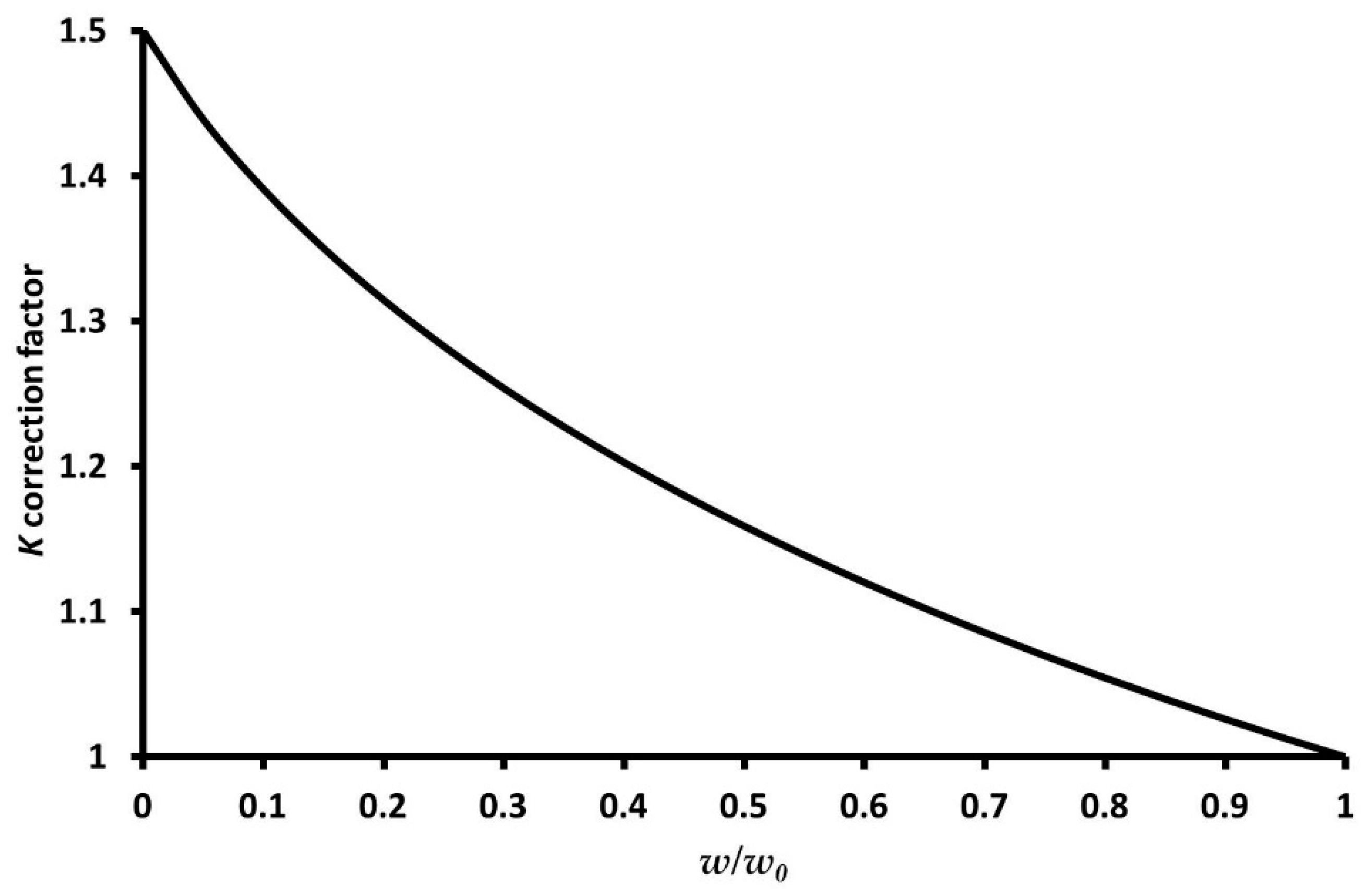
3.1. Correction Factor for Euler Beam Equation for Plan-View Trapezoidal Cantilevers

Figure 1 defines the plan-view parameters for a trapezoidal cantilever, and we assume the cantilever has a uniform thickness, t. The base width of the cantilever is w₀ and the top width is w.

We shall use the same nomenclature as used by Sader and White [1]. Therefore, Equation A3a in Sader and White [1] describes the equation for the angled side of the trapezoidal cantilever and is given by:

y = f(x) = a(1 − mx) = a − amx

(4)

where Sader and White [1] define a and m as adjustable gradient parameters. Therefore, the y-intercept for this function is the variable a, and the absolute value of the slope of the function is am.

We can see from Figure 1 that half the base width of the cantilever equals to a (i.e., a = w₀/2) and the slope of the angled side equals to (w₀ − w)/(2L). Therefore, am = (w₀ − w)/(2L), and given a = w₀/2, then m = (w₀ − w)/(Lw₀). Sader and White [1] derived the following formula (which is Equation A3b in their article) for a trapezoidal cantilever:

k = 2(D’am³)/(mL − 1)[mL − m²L²/(2(1 − mL)) + (1 − mL)ln(1 + mL)]⁻¹

(5)

where D’ = E_ct³/12

Therefore, if we substitute a = w₀/2, m = (w₀ − w)/(Lw₀), and D’ = E_ct³/12 into Equation (5), it can be rewritten as:

K = (E_ct³w₀/(4L³))·[(w/w₀ − 1)³/(3w/w₀) ((1 − w/w₀) − (1 − w/w₀)²/(2w/w₀) + (w/w₀) ln(w/w₀))⁻¹]

(6)

If we let K = 3(w/w₀)/(w/w₀ − 1)³((1 − w/w₀) − (1 − w/w₀)²/(2w/w₀) + (w/w₀)ln(w/w₀)), then we can rewrite Equation (6) as

k = E_ct³w₀/(4KL³)

(7)

For AFM cantilevers, where the tip is offset from the very end of the cantilever L = L_tip.

Therefore, the K term can also be considered a correction factor to the Euler beam equation (given in Equation (1)), which is dependent on the ratio of the top width to the base width, i.e., w/w₀ for trapezoidal cantilevers. We can, therefore, plot K versus w/w₀, and this is displayed in Figure 2.

An advantage of the calibration curve in Figure 2 is that it relies on the ratio of w/w₀ which means that any error in the calibration of the instrument measuring w or w₀ will effectively cancel. For practical cantilevers with a trapezoidal plan-view, the width, w, should be measured through the tip apex position since this is where the force is applied to the cantilever when in operation. Figure 3 shows a plan-view SEM image of a trapezoidal-shaped cantilever (Bruker FastScan C) with the dimensions w₀, w, L and L_tip defined.

It should be noted that an engineering text authored by Robert E. Joeress [57] also has a correction factor versus w/w₀ graph for plan-view trapezoidal cantilevers displayed in Figure 6.43 of the Joeress text [57]. A comparison between our data in Figure 2 and the data plotted in Joeress [57] graph shows a maximum difference of approximately 1.6%. However, it is also important to note that for the calibration curve displayed in the Joeress [57] work, there are no details given on how their plot was generated. Given that the analysis performed in this work is traceable to established analytical calculations, the authors recommend using Equation (6), or Equation (7) combined with Figure 2, to determine the spring constant of trapezoidal cantilevers.

If the spring constant of the cantilever is determined using another experimental technique (e.g., refs [16,17,18,19,20,21,22,23,24,25,26,27,28,29,30,31,32,33]) and the dimensions are determined using SEM, for example, then Equation (7) can also be used to determine Young’s modulus of the AFM cantilever or indeed any cantilevered structure with a trapezoidal plan view, provided w is less than w₀. This technique has been used to determine Young’s modulus of wool fibres and polymer actuators [58,59].

3.2. Deriving Solutions to the Torque Correction Factor for Plan-View Triangular and Trapezoidal Cantilevers

Edwards et al. [55] defines the general expression for determining the torque, T_i, for a cantilever of arbitrary shape with a sharp tip, and we use the same notation that Edwards et al. [55] use in their work. It is given as:

T_i = 1 − ρ_i (tanα)D

(8)

where i refers to z or θ, which are the normal and longitudinal directions of the cantilever, respectively. The torque we are interested in is the normal direction therefore T_z is the correction factor we focus on for the various plan-view geometries. The term ρ_i (Equation (17) from Edwards et al. [55]) can be expressed as:

ρ_z = k_z/k_zθ

(9)

where k_z is the normal spring constant for the cantilever, and k_zθ is the longitudinal spring constant of the cantilever. For a beam-shaped cantilever, we get k_z from Equation (1) and k_zθ (Edwards et al. [55]) is defined as:

k_zθ = E_ct³w/(6L²)

(10)

So if we divide k_z by k_zθ for a beam-shaped cantilever we can obtain ρ_z. If we then substitute the result of k_z/k_zθ back into Equation (8), we get the familiar term for the torque for a beam-shaped cantilever, T_beam, which is given in Equation (3).

For a trapezoidal cantilever, the situation is more complex since while we have an expression for k_z for a trapezoidal cantilever (refer to Equations (6) and (7)), we do not have one for k_zθ. However, we can assume that the torque, T_trap., for a trapezoidal cantilever will be in between that for a beam-shaped cantilever, T_beam, and a triangular-shaped cantilever, T_tri., with the same base width, w₀, and length, L. This is represented in Figure 4.

Therefore, if we determine T_beam and T_tri., we can determine an upper and lower limit for T_trap. Firstly, we require k_z for a triangular cantilever. From Equation A2a and A2b from Sader and White [1], we can express k_z for a triangular cantilever as:

k_z = E_ct³w₀/(6L³)

(11)

The term w₀ is now the width of the base of the triangular cantilever. Alternatively, we could use Equation (6) or simply refer to Figure 2 since when w/w₀ approaches zero, we see that the K correction factor will approximate to 1.5. If we substitute 1.5 into Equation (7), we obtain the expression shown in Equation (11). After extensive searching, the authors could not find a simple expression for k_zθ for a triangular cantilever in the literature. However, in the article by Sader [40], they derive an equation for k_zθ for a V-shaped cantilever. This Equation is 3b in the article [40] and is as follows:

k_zθ = E_ct³w₀/(12L²) [2w_a/w₀ − ΔL/L(1 + log((2w_a/w₀) (ΔL/L))) + Π (w₀/2w_a − 1)(1/2 + w₀/2w_a − ΔL/L)]

(12)

where w_a is now the width of one of the arms of the V-shaped cantilever, and w₀ is the overall base width of the cantilever. In Sader [40], the term Π is expressed as:

Π = (1 + ν)/((Γ²(2 − [1 − ν]Γ²))

(13)

where ν is the Poisson’s ratio for the cantilever material and Γ is given by

Γ = (1 + w_a²/(4L²))^−0.5

(14)

This can be simplified further if we assume the length, L, of the cantilever is from the base to the tip apex and we ignore the additional length of the cantilever from the tip apex to the very end of the beam. As mentioned, this is reasonable as the extra length has no impact on the torque since the AFM tip apex is where the force or torque is being applied. This means we can effectively assume ΔL = 0 and L = L_tip, and therefore, Equation (12) can be simplified to:

k_zθ = E_ct³w₀/12L_tip² [2w_a/w₀ + Π (w₀/2w_a − 1)(1/2 + w_a/w₀)]

(15)

As the width of the arms of the cantilever, w_a, approaches w₀/2, the V-shaped cantilever approaches a closed triangular shape as shown in Figure 5.

Therefore, if we assume that w_a = w₀/2, and substitute this into Equation (14), it will simplify to:

k_zθ = E_ct³w₀/(12L_tip²)

(16)

We now have equations for k_z and k_zθ for a triangular cantilever. We can now determine ρ_z for a triangular cantilever using Equation (9), and then using that value determine T_tri. for the triangular cantilever using Equation (8). Doing this results in the expression:

T_tri. = 1 − (tanα)(2(D/L_tip))

(17)

We can assume that the torque for a trapezoidal cantilever will be between T_rect. and T_tri., or to simplify this, we shall simply average Equations (3) and (16). We, therefore, approximate the torque produced by the AFM tip for a trapezoidal cantilever as:

T_trap. ≈ 1 – (tanα)(7/4)(D/L_tip)

(18)

3.3. Application of Derived Expressions

There is minimal experimental data available in the literature measuring D/L_tip for different cantilever types. There are, however, two sources of such data for relatively short FastScan cantilevers. The first was published by Song et al. [49] and the second provided by Slattery et al. [43]. Table 1 provides details of 11 cantilevers and includes dimensions, data on the height of the tips, as well as the D/L_tip ratio, the torque factors, T_beam, T_tri. and T_trap., and the Euler correction factors, K. The approach angle, α, used to calculate the torque corrections is 12⁰. The details of the first four cantilevers (FSA1–4) are from Song et al. [49] and are for cantilevers from the same wafer. Dimensional data for cantilevers FSA5–7, FSB1–2, and FSC1–2 are provided by the authors and the spring constant data for cantilevers which have been previously reported by Slattery et al. [43].

A number of important insights into the cantilever geometry and spring constant could be determined from Table 1. The w/w₀ ratio is less than 0.5 for all cantilever types which indicates that while they all have a trapezoidal plan-view shape, they are closer to a triangular shape than beam-shaped. This has interesting results for each of the Euler beam and torque correction factors discussed in this work. For the Euler beam correction factor, K, we can see that if we simply assume a triangular shape, then K = 1.5 and the spring constant for the cantilevers will be underestimated by 13 to 20%, while for the torque correction factors if the beam shape was used compared to the triangular, the extreme limits for the plan-view shape, we see a difference of only 3%. This indicates that for the torque correction factor, the plan-view shape has a much weaker dependence than for the Euler beam formula. Therefore given that all cantilevers are closer to a triangular shape, either the triangular torque correction (Equation (16)) or the trapezoidal approximation (Equation (17)) would be suitable.

However Table 1 does show that the torque factor, regardless of plan-view shape, for these cantilevers is significant and if not accounted for, could lead to errors of up to ~11%. The variation in tip height, D, is significant between probes of different types but also between probes of the same type. For example, the probes, FSA1–4, are from the same batch and show a difference in tip height from 4.55 to 7.03 μm. This results in T_trap. values varying from 0.89 to 0.95 for these probes. The K correction factor is similar for probes of the same type but does show some change between types and reflects that the plan-view geometry for each cantilever model is generally consistent.

What is also interesting to note is how much stiffer cantilever FSA6 is compared to the other FastScan A cantilevers. It is between 30 to 60% stiffer than the other FSA cantilevers despite having similar dimensions and tip height. The most likely reason is the difference between the length of the cantilever from the base to the tip apex, L_tip. The spring constant values reported in Table 1 used methods that determine the spring constant of the cantilever at the tip apex and if we compare L_tip for cantilever FSA6 to the other cantilevers, we see that this dimension is on average 11 to 20% smaller. Given there is an inverse cubic relationship between cantilever spring constant and L_tip (refer to Equations (1) and (2)), then it is not surprising that FSA6 is significantly stiffer than the other FSA probes. While the absolute difference between the L_tip for FSA6 and the other FSA cantilevers is only a few microns, this becomes more significant to the spring constant the shorter the cantilever becomes. Therefore, methods that determine the spring constant at the tip apex have an advantage. For methods that do not determine the spring constant at the tip apex, such as those that rely on measuring the resonant frequency of the cantilever, care must be taken to accurately determine L and L_tip and then use Equation (2) to account for this effect. Indeed, the smaller AFM cantilevers become the more important this effect will be and should be noted by all AFM users intending to perform accurate force measurements using small cantilevers.

To apply the analysis in Section 3.1 and Section 3.2, we use the results from Table 1 and Equation (6) to determine Young’s modulus of each of the cantilevers in Table 1. We report the effective Young’s modulus, but also Young’s modulus of silicon nitride the cantilevers are composed of. To determine Young’s modulus for the silicon nitride required for correcting the effective Young’s modulus values for the metal coatings on the back of the cantilevers using equations derived by Sader et al. [53]. This data is displayed in

Table 2. Shows the spring constant, effective Young’s modulus of the cantilevers, and Young’s modulus of the silicon nitride the cantilevers are composed of which has been corrected for the thin metal coatings on the back of the cantilevers using equations derived by Sader et al. [53].

AFM Probe	Spring Constant (N/m)	Effective Young’s Modulus of Cantilever (GPa)	Silicon Nitride Young’s Modulus of Cantilever (GPa)
FSA1	15.81	201.3	229.2
FSA2	14.24	210.1	240.6
FSA3	17.05	151.9	168.3
FSA4	11.89	216.4	238.9
FSA5	21.4	155	171
FSA6	32.3	161	178
FSA7	18.5	132	143
FSB1	2.24	161	177
FSB2	2.05	164	181
FSC1	0.938	204	230
FSC2	0.916	212	241

, and for reference shows the spring constant values for each cantilever as reported in Table 1.

The results in Table 2 show an average effective Young’s modulus and silicon nitride Young’s modulus of 179 ± 29 and 200 ± 34 GPa, respectively for all the cantilevers, with the error quoted representing one standard deviation in the data. The average Young’s modulus for the silicon nitride is in excellent agreement with the value provided to the authors by the manufacturer, which is 200 GPa. The values also fit within the range determined by Drummond et al. [50] who reported Young’s modulus for silicon nitride in the cantilevers they analysed to be, on average, 202 ± 45 GPa. Bader [60] also reported Young’s modulus for micromechanical cantilevers made from silicon nitride equal to 194 ± 14 GPa, which is in good agreement with our average value for silicon nitride. This suggests the effective application of the method and correction factors derived in this work.

Further analysis can reveal how robust Equation (6) is if we use the 179 GPa result and default values for k, L_tip, w₀ provided by the manufacturer for each type of FastScan probe, and then determine the thickness using Equation (6). If the cantilever thickness we calculate is within 10% of the default value quoted by the manufacturer, then our Equation (6) can be considered acceptably accurate. Default values for each cantilever type are provided in Table S1 of the Supplementary material. Our analysis reveals that for FastScan A cantilevers, we obtain a thickness measurement of 0.54 μm and the default value provided by the manufacturer for the thickness is 0.58 μm. This is a difference of 6.9% compared to the default value. The same analysis for the FastScan B cantilevers gives a thickness of 0.29 μm using our equation compared to 0.30 μm, which is the default value quoted by the manufacturer for FastScan B probes. This is a 3.3% difference. The same analysis for the FastScan C cantilevers gives a thickness of 0.31 μm using our equation compared to 0.30 μm, which is the default value for the thickness quoted by the manufacturer for FastScan C probes. This is a 3.3% difference, suggesting sufficient overall accuracy for successful practical application.

Slattery et al. [43] also demonstrated that the spring constant calibration of smaller cantilevers is more challenging than standard larger AFM cantilevers. This is particularly true for the FastScan A model, which is the smallest and stiffest of the FastScan cantilever models. Slattery et al. [43] showed that the thermal noise method, often built-in to modern AFM instruments, overestimated the spring constant of FastScan A cantilevers significantly (30 to 70%). This was attributed to the reduced thermal noise profile for these types of probes, and this effect has been observed by other research groups [24]. Therefore, we have applied the Sader indirect method [16,34] to the calibration of the spring constant of the FastScan A cantilevers reported in this work. In the Sader indirect method [16], typically the spring constant of one cantilever is accurately measured and then the term E_ct³ is determined using an appropriate Euler beam equation, based on the cantilever plan-view geometry. This E_ct³ value is then assumed to be constant for all cantilevers of the same type and subsequent cantilevers can then be calibrated with only the length and width of the cantilever requiring measurement. In our case, we use a slightly different approach. We have already determined an average effective Young’s modulus, E_c, for FastScan cantilevers of 179 ± 29 GPa. We, therefore, determine an average cantilever thickness, t, for the FastScan A probes from the data presented in Table 1, which gives 0.60 ± 0.04 μm, with the error quoted being one standard deviation in the data. Combining this with E_c gives us an E_ct³ value of 3.87 ± 0.97 × 10⁻⁸ Nm for our FastScan A probes. The uncertainty on the E_ct³ term is approximately 25% and has contributions from the uncertainty on the E_c term and the uncertainty on the average thickness for the FastScan A probes, t, which is a cubed term. We have used this E_ct³ value to then calculate the spring constant of FastScan A cantilevers FSA1–7. The Sader indirect method [16] results are reported in

Table 3. Shows a comparison between the spring constant of the FastScan A cantilevers determined using the methods described in Slattery et al. [43] and Song et al. [49] and the Sader indirect method [16].

AFM Probe	Spring Constant (N/m)	Sader Indirect Method (N/m)
FSA1	15.81	15.5
FSA2	14.24	14.1
FSA3	17.05	19.0
FSA4	11.89	11.9
FSA5	21.4	19.1
FSA6	32.3	27.3
FSA7	18.5	19.7

and compared to the more accurate spring constant values cantilevers as reported by Song et al. [49] and Slattery et al. [43].

The agreement between the accurate spring constant values and the Sader indirect method is good with all Sader indirect results being within 2 to 15% of the accurate values. Therefore, the E_ct³ value determined in this work could be used by other groups to calibrate the spring constant of the FastScan A cantilevers with the proviso that the uncertainty of the spring constants using this method could be as high as 25% given the uncertainty on the E_ct³ term calculated in this work.

4. Discussion

In this work, we have derived a simple correction factor to the Euler beam equation for beam-shaped cantilevers which allows the spring constant of trapezoidal plan-view shaped cantilevers to be determined (provided the material properties and dimensions are known). The derivation for this correction factor, K, is based on the analytical work by Sader and White [1]. We have also derived simple expressions for the torque correction factor for triangular plan-view shaped cantilevers, as well as an approximation for the torque correction for trapezoidal plan-view shaped cantilevers. The torque corrections were based on the work by Edwards et al. [55] and Sader [40].

Analysis of the spring constant and dimensions of 11 Bruker FastScan AFM probes revealed that the K correction factor was between 1.2 and 1.31, which is a significant correction given that K =1 for a beam-shaped cantilever and K = 1.5 for a triangular-shaped cantilever. The torque correction factors for the FastScan cantilevers were significant, and if not accounted for could introduce errors as high as ~11%. However, the torque corrections did show a much weaker dependence on the plan-view geometry, and there was, at maximum, only a 3% difference between the torque correction factors for a beam-shaped cantilever and a triangular-shaped cantilever for the same cantilever. However, given w/w₀ is less than 0.5 for all FastScan cantilevers studied in this work we would expect the triangular torque correction, or the trapezoidal approximation, to be suitable for Bruker FastScan cantilevers. It is also important to note that as AFM cantilevers become smaller the D/L_tip ratio will increase, and the plan-view shape of the cantilever will play a more important role in determining which torque correction factor is the most appropriate to use.

Close analysis of the different dimensions for the shortest cantilever type (FastScan A) indicated that the L_tip dimension is crucial in contributing to the variability in the spring constant for these types of AFM probes. This is due to the inverse cubic relationship between L_tip and the cantilever spring constant (refer to Equations (1) and (2)) and indicates that the smaller AFM cantilevers become the more significant L_tip will become. This will impact methods that do not calibrate the spring constant of the cantilever at the tip apex such as those based on the resonant frequency of the cantilever. For these techniques, the precise measurement of L and L_tip will be required.

We also applied the derived correction factors to determine Young’s modulus of 11 Bruker FastScan AFM probes. Our results gave an average Young’s modulus for the silicon nitride the cantilevers are composed of equal to 200 ± 34 GPa which is comparable to the results reported by other research groups [50,60], and equal to that quoted to us by the manufacturer. We also applied the Sader indirect [16] method to calibrate the FastScan A type cantilevers and found good agreement between the Sader indirect [16] method and the more precise results reported by Slattery et al. [43] and Song et al. [49] for these probes. This will be useful for AFM users as research has shown that some standard methods, such as the thermal noise method, struggle to provide accurate results for these types of AFM probes.

References

1. Sader, J.E.; White, L. Theoretical analysis of the static deflection of plates for atomic force microscope applications. J. Appl. Phys. 1993, 74, 1–9. [Google Scholar] [CrossRef] [Green Version]
2. Steffens, C.; Leite, F.L.; Bueno, C.C.; Manzoli, A.; Herrmann, P.S.D.P. atomic force microscopy as a tool applied to nano/biosensors. Sensors 2012, 12, 8278–8300. [Google Scholar] [CrossRef] [PubMed]
3. Creasey, R.; Sharma, S.; Craig, J.E.; Gibson, C.T.; Ebner, A.; Hinterdorfer, P.; Voelcker, N.H. Detecting protein aggregates on untreated human tissue samples by atomic force microscopy recognition imaging. Biophys. J. 2010, 99, 1660–1667. [Google Scholar] [CrossRef] [PubMed]
4. Da Silva, A.C.N.; Deda, D.K.; Da Róz, A.L.; Prado, R.A.; Carvalho, C.C.; Viviani, V.; Leite, F.L. Nanobiosensors based on chemically modified afm probes: a useful tool for metsulfuron-methyl detection. Sensors 2013, 13, 1477–1489. [Google Scholar] [CrossRef]
5. Creasey, R.; Sharma, S.; Gibson, C.T.; Craig, J.E.; Ebner, A.; Becker, T.; Hinterdorfer, P.; Voelcker, N.H. Atomic force microscopy-based antibody recognition imaging of proteins in the pathological deposits in pseudoexfoliation syndrome. Ultramicroscopy 2011, 111, 1055–1061. [Google Scholar] [CrossRef]
6. Zdunek, A.; Kurenda, A. Determination of the elastic properties of tomato fruit cells with an atomic force microscope. Sensors 2013, 13, 12175–12191. [Google Scholar] [CrossRef]
7. Crossley, J.A.A.; Gibson, C.T.; Mapledoram, L.D.; Huson, M.G.; Myhra, S.; Pham, D.K.; Sofield, C.J.; Turner, P.S.; Watson, G.S. Atomic force microscopy analysis of wool fibre surfaces in air and under water. Micron 2000, 31, 659–667. [Google Scholar] [CrossRef]
8. Goreham, R.V.; Thompson, V.C.; Samura, Y.; Gibson, C.T.; Shapter, J.G.; Köper, I. Interaction of silver nanoparticles with tethered bilayer lipid membranes. Langmuir 2015, 31, 5868–5874. [Google Scholar] [CrossRef]
9. Bowen, W.R.; Lovitt, R.W.; Wright, C.J. Application of atomic force microscopy to the study of micromechanical properties of biological materials. Biotechnol. Lett. 2000, 22, 893–903. [Google Scholar] [CrossRef]
10. Shearer, C.J.; Slattery, A.D.; Stapleton, A.J.; Shapter, J.G.; Gibson, C.T. Accurate thickness measurement of graphene. Nanotechnology 2016, 27, 125704. [Google Scholar] [CrossRef]
11. Lavrik, N.V.; Sepaniak, M.J.; Datskos, P.G. Cantilever transducers as a platform for chemical and biological sensors. Rev. Sci. Instrum. 2004, 75, 2229–2253. [Google Scholar] [CrossRef]
12. Raiteri, R.; Grattarola, M.; Butt, H.J.; Skladal, P. Micromechanical cantilever-based biosensors. Sens. Actuat. B Chem. 2001, 79, 115–126. [Google Scholar] [CrossRef]
13. Cleveland, J.P.; Manne, S.; Bocek, D.; Hansma, P.K. A nondestructive method for determining the spring constant of cantilevers for scanning force microscopy. Rev. Sci. Instrum. 1993, 64, 403–405. [Google Scholar] [CrossRef] [Green Version]
14. Sader, J.E. Parallel beam approximation for V-shaped atomic force microscope cantilevers. Rev. Sci. Instrum. 1995, 66, 4583–4587. [Google Scholar] [CrossRef]
15. Poggi, M.A.; McFarland, A.W.; Colton, J.S.; Bottomley, L.A. A method for calculating the spring constant of atomic force microscopy cantilevers with a nonrectangular cross section. Anal. Chem. 2005, 77, 1192–1195. [Google Scholar] [CrossRef] [PubMed]
16. Sader, J.E.; Chon, J.W.M.; Mulvaney, P. Calibration of rectangular atomic force microscope cantilevers. Rev. Sci. Instrum. 1999, 70, 3967–3969. [Google Scholar] [CrossRef] [Green Version]
17. Sader, J.E.; Sanelli, J.A.; Adamson, B.D.; Monty, J.P.; Wei, X.; Crawford, S.A.; Friend, J.R.; Marusic, I.; Mulvaney, P.; Bieske, E.J. Spring constant calibration of atomic force microscope cantilevers of arbitrary shape. Rev. Sci. Instrum. 2012, 83, 103705. [Google Scholar] [CrossRef] [PubMed] [Green Version]
18. Sader, J.E.; Friend, J.R. Calibration of atomic force microscope cantilevers using only their resonant frequency and quality factor. Rev. Sci. Instrum. 2014, 85, 116101. [Google Scholar] [CrossRef]
19. Sader, J.E.; Borgani, R.; Gibson, C.T.; Haviland, D.B.; Higgins, M.J.; Kilpatrick, J.I.; Lu, J.; Mulvaney, P.; Shearer, C.J.; Slattery, A.D.; et al. A virtual instrument to standardise the calibration of atomic force microscope cantilevers. Rev. Sci. Instrum. 2016, 87, 093711. [Google Scholar] [CrossRef]
20. Slattery, A.D.; Quinton, J.S.; Gibson, C.T. Atomic force microscope cantilever calibration using a focused ion beam. Nanotechnology 2012, 23, 285704. [Google Scholar] [CrossRef]
21. Golovko, D.S.; Haschke, T.; Wiechert, W.; Bonaccurso, E. Nondestructive and noncontact method for determining the spring constant of rectangular cantilevers. Rev. Sci. Instrum. 2007, 78, 043705. [Google Scholar] [CrossRef] [PubMed]
22. Cook, S.; Schaffer, T.E.; Chynoweth, K.M.; Wigton, M.; Simmonds, R.W.; Lang, K.M. Practical implementation of dynamic methods for measuring atomic force microscope cantilever spring constants. Nanotechnology 2006, 17, 2135–2145. [Google Scholar] [CrossRef] [Green Version]
23. Lévy, R.; Maaloum, M. Measuring the spring constant of atomic force microscope cantilevers: Thermal fluctuations and other methods. Nanotechnology 2002, 13, 33. [Google Scholar] [CrossRef]
24. Ohler, B. Cantilever spring constant calibration using laser Doppler vibrometry. Rev. Sci. Instrum. 2007, 78, 063701. [Google Scholar] [CrossRef] [PubMed]
25. Gates, R.S.; Pratt, J.R. Accurate and precise calibration of AFM cantilever spring constants using laser Doppler vibrometry. Nanotechnology 2012, 23, 375702. [Google Scholar] [CrossRef]
26. Slattery, A.D.; Blanch, A.J.; Quinton, J.S.; Gibson, C.T. Accurate measurement of atomic force microscope cantilever deflection excluding tip-surface contact with application to force calibration. Ultramicroscopy 2013, 131, 46–55. [Google Scholar] [CrossRef]
27. Burnham, N.A.; Chen, X.; Hodges, C.S.; Matei, G.A.; Thoreson, E.J.; Roberts, C.J.; Davies, M.C.; Tendler, S.J.B. Comparison of calibration methods for atomic-force microscopy cantilevers. Nanotechnology 2003, 14, 1. [Google Scholar] [CrossRef]
28. Slattery, A.D.; Blanch, A.J.; Quinton, J.S.; Gibson, C.T. Calibration of atomic force microscope cantilevers using standard and inverted static methods assisted by FIB-milled spatial markers. Nanotechnology 2013, 24, 015710. [Google Scholar] [CrossRef]
29. Clifford, C.A.; Seah, M.P. Improved methods and uncertainty analysis in the calibration of the spring constant of an atomic force microscope cantilever using static experimental methods. Meas. Sci. Technol. 2009, 20, 125501. [Google Scholar] [CrossRef]
30. Kim, M.-S.; Choi, J.-H.; Kim, J.-H.; Park, Y.-K. Accurate determination of spring constant of atomic force microscope cantilevers and comparison with other methods. Measurement 2010, 43, 520–526. [Google Scholar] [CrossRef]
31. Cumpson, P.J.; Clifford, C.A.; Hedley, J. Quantitative analytical atomic force microscopy: A cantilever reference device for easy and accurate AFM spring-constant calibration. Meas. Sci. Technol. 2004, 15, 1337–1346. [Google Scholar] [CrossRef]
32. Gates, R.S.; Reitsma, M.G. Precise atomic force microscope cantilever spring constant calibration using a reference cantilever array. Rev. Sci. Instrum. 2007, 78, 086101. [Google Scholar] [CrossRef] [PubMed]
33. Senden, T.; Ducker, W. Experimental determination of spring constants in atomic force microscopy. Langmuir 1994, 10, 1003–1004. [Google Scholar] [CrossRef]
34. Gibson, C.T.; Johnson, D.J.; Anderson, C.; Abell, C.; Rayment, T. Method to determine the spring constant of atomic force microscope cantilevers. Rev. Sci. Instrum. 2004, 75, 565–567. [Google Scholar] [CrossRef]
35. Shatil, N.R.; Homer, M.E.; Picco, L.; Martin, P.G.; Payton, O.D. A calibration method for the higher modes of a micro-mechanical cantilever. Appl. Phys. Lett. 2017, 110, 223101. [Google Scholar] [CrossRef] [Green Version]
36. Payam, A.F.; Trewby, W.; Voitchovsky, K. Determining the spring constant of arbitrarily shaped cantilevers in viscous environments. Appl. Phys. Lett. 2018, 112, 083101. [Google Scholar] [CrossRef] [Green Version]
37. Cafolla, C.; Payam, A.F.; Voitchovsky, K. A non-destructive method to calibrate the torsional spring constant of atomic force microscope cantilevers in viscous environments. J. Appl. Phys. 2018, 124, 154502. [Google Scholar] [CrossRef] [Green Version]
38. Labuda, A.; Cao, C.; Walsh, T.; Meinhold, J.; Proksch, R.; Sun, Y.; Filleter, T. Static and dynamic calibration of torsional spring constants of cantilevers. Rev. Sci. Instrum. 2018, 89, 093701. [Google Scholar] [CrossRef] [Green Version]
39. Thoren, P.-A.; Borgani, R.; Forcheimer, D.; Haviland, D.B. Calibrating torsional eigenmodes of micro-cantilevers for dynamic measurement of frictional forces. Rev. Sci. Instrum. 2018, 89, 075004. [Google Scholar] [CrossRef] [Green Version]
40. Sader, J.E. Susceptibility of atomic force microscope cantilevers to lateral forces. Rev. Sci. Instrum. 2003, 74, 2438–2443. [Google Scholar] [CrossRef] [Green Version]
41. Sader, J.E.; Sader, R.C. Susceptibility of atomic force microscope cantilevers to lateral forces: Experimental verification. Appl. Phys. Lett. 2003, 83, 3195–3197. [Google Scholar] [CrossRef]
42. Ando, T.; Uchihashi, T.; Kodera, N.; Yamamoto, D.; Miyagi, A.; Taniguchi, M.; Yamashita, H. High-speed AFM and nano-visualization of biomolecular processes. Pflug. Arch. 2008, 456, 211–225. [Google Scholar] [CrossRef] [PubMed]
43. Slattery, A.D.; Blanch, A.J.; Ejov, V.; Quinton, J.S.; Gibson, C.T. Spring constant calibration techniques for next-generation fast-scanning atomic force microscope cantilevers. Nanotechnology 2014, 25, 335705. [Google Scholar] [CrossRef] [PubMed]
44. Morshed, S.; Prorok, B.C. Tailoring beam mechanics towards enhancing detection of hazardous biological species. Exp. Mech. 2007, 47, 405–415. [Google Scholar] [CrossRef]
45. Zhao, J.; Zhang, Y.; Gao, R.; Liu, S. A new sensitivity improving approach for mass sensors through integrated optimization of both cantilever profile and cross-section. Sens. Actuators B Chem. 2015, 206, 343–350. [Google Scholar] [CrossRef]
46. Longqi, X.; Guiming, Z.; Libo, Z.; Yulong, Z.; Zhuangde, J.; Rahman, H.; Hongyan, W.; Zhigang, L. A fluid viscosity sensor with resonant trapezoidal micro cantilever. IEEE Int. Symp. Assem. Manuf. (ISAM) 2013, 131–134. [Google Scholar]
47. Zhao, L.-B.; Xu, L.-Q.; Zhang, G.-M.; Zhao, Y.-L.; Wang, X.-P.; Liu, Z.-G.; Jiang, Z.-D. A trapezoidal cantilever density sensor based on MEMS technology. J. Zhejiang Univ. Sci. C 2013, 14, 274–278. [Google Scholar] [CrossRef]
48. Huang, W.; Kwon, S.-R.; Zhang, S.; Yuan, F.-G.; Jiang, X. A trapezoidal flexoelectric accelerometer. J. Intell Mater. Syst Struct. 2014, 25, 271–277. [Google Scholar] [CrossRef]
49. Song, Y.-P.; Wu, S.; Xu, L.-Y.; Zhang, J.-M.; Dorantes-Gonzalez, D.J.; Fu, X.; Hu, X.-D. Calibration of the effective spring constant of ultra-short cantilevers for a high-speed atomic force microscope. Meas. Sci. Technol. 2015, 26, 065001. [Google Scholar] [CrossRef]
50. Drummond, C.J.; Senden, T.J. Characterisation of the mechanical properties of thin film cantilevers with the atomic force microscope. Mater Sci. Forum 1995, 189, 107–114. [Google Scholar] [CrossRef]
51. Bean, K.E.; Gleim, P.S.; Yeakley, R.L.; Runyan, W.R. Some properties of vapor deposited silicon nitride films using the SiH4-NH3-H2 system. J. Electrochem. Soc. 1967, 114, 733–737. [Google Scholar] [CrossRef]
52. Tai, Y.C.; Muller, R.S. Measurement of Young’s modulus on microfabricated structures using a surface profiler. Proc. IEEE Micro. Electro. Mechanical Syst. 1990, 147. [Google Scholar]
53. Sader, J.E.; Larson, I.; Mulvaney, P.; White, L.R. Method for the calibration of atomic force microscope cantilevers. Rev. Sci. Instrum. 1995, 66, 3789–3798. [Google Scholar] [CrossRef] [Green Version]
54. Albrecht, T.R.; Akamine, S.; Carver, T.E.; Quate, C.F. Microfabrication of cantilever styli for the atomic force microscope. J. Vac. Sci. Technol. A. 1990, 8, 3386–3396. [Google Scholar] [CrossRef]
55. Edwards, S.A.; Ducker, W.A.; Sader, J.E. Influence of atomic force microscope cantilever tilt and induced torque on force measurements. J. Appl. Phys. 2008, 103, 064513. [Google Scholar] [CrossRef] [Green Version]
56. Cumpson, P.J.; Hedley, J. Accurate analytical measurements in the atomic force microscope: A microfabricated spring constant standard potentially traceable to the SI. Nanotechnology 2003, 14, 1279–1288. [Google Scholar] [CrossRef]
57. Joerres, R.E. Machine elements that absorb and store energy. In Standard Handbook of Machine Design; Shigley, J., Ed.; McGraw-Hill: New York, NY, USA, 2004; pp. 1–70. [Google Scholar]
58. Gibson, C.T.; Myhra, S.; Watson, G.S.; Huson, M.G.; Pham, D.K.; Turner, P.S. Effects of aqueous exposure on the mechanical properties of wool fibers—Analysis by atomic force microscopy. Text. Res. J. 2001, 71, 573–581. [Google Scholar] [CrossRef]
59. Alici, G.; Higgins, M. Normal stiffness calibration of microfabricated tri-layer conducting polymer actuators. Smart Mater. Struct. 2009, 18, 065013. [Google Scholar] [CrossRef]
60. Bader, S. Characterization of silicon nitride micromechanical cantilevers and bridges. J. Micro/Nano Process. Technol. 2013, 3, 1–3. [Google Scholar]
Figure 1. Schematic of the top-down view of a trapezoidal cantilever using the same notation as Sader and White [1].
Applsci 09 02604 g001
Figure 2. A calibration curve for trapezoidal plan-view cantilevers. The correction factor, K, can be determined from the w/w0, and then substituted into Equation (7) to determine the cantilever spring constant.
Applsci 09 02604 g002
Figure 3. Plan-view SEM image of trapezoidal-shaped Bruker FastScan C cantilever.
Applsci 09 02604 g003
Figure 4. Shows that the trapezoidal cantilever shape, given in Figure 4b, is a trapezoidal shaped cantilever with base width wo and top width w. Its geometry is in between that for a beam-shaped cantilever (a) and a triangular cantilever (c) with the same base width w0.
Applsci 09 02604 g004
Figure 5. Shows how a V-shaped cantilever, depicted in (a) with arm width wa and overall base width wo, approximates a triangular cantilever with the same overall base width wo, depicted in (b), as the arm width of the V-shaped cantilever, wa approaches w0/2. or 2wa = wo.
Applsci 09 02604 g005