Abstract
Firefly algorithm is among the nature-inspired optimization algorithms. The standard firefly algorithm has been successfully applied to many engineering problems. However, this algorithm might be stuck in stagnation (the solutions do not enhance anymore) or possibly fall in premature convergence (fall into the local optimum) in searching space. It seems that both issues could be connected to exploitation and exploration. Excessive exploitation leads to premature convergence, while excessive exploration slows down the convergence. In this study, the classical firefly algorithm is modified such that make a balance between exploitation and exploration. The purposed modified algorithm ranks and sorts the initial solutions. Next, the operators named insertion, swap and reversion are utilized to search the neighbourhood of solutions in the second group, in which all these operators are chosen randomly. After that, the acquired solutions combined with the first group and the firefly algorithm finds the new potential solutions. A multi-echelon supply chain network problem is chosen to investigate the decisions associated with the distribution of multiple products that are delivered through multiple distribution centres and retailers and demonstrate the efficiency of the proposed algorithm.
1. Introduction
Firefly Algorithm (FA), initially introduced by Yang [1], is a nature-inspired algorithm originated from the flashing lights of fireflies. FA is among the latest swarm intelligence techniques and it is among metaheuristic algorithms and stochastic optimization approaches which can be applied for many difficult engineering problems including NP-Hard problems [2,3]. According to computational complexity theory, there are four types of problems based on their inherent difficulty. These problems comprise P, NP, NP-Complete and NP-Hard problem (interested may refer to [2,3] for more information). FA searches for a set of solutions by using a kind of randomization which means that it belongs to stochastic algorithms.
Flashing lights are the main characteristic of fireflies. The flashing lights have two primary functions: to attract mating partners and to warn other fireflies of probable predators. The flashing lights follow laws of physics, that is, according to the term, when the distance r increase, the intensity of flashing lights I decrease. This phenomenon inspired Yang [1] to develop the FA. The classical FA was numerically formulated and implemented in MATLAB and it was explained in detail in Yang (2008) and Yang (2009).
There are two key factors need to be well defined to design FA properly: the formulation of attractiveness and the variation of light intensity. In FA, the light intensity (I) of a firefly, that presents the solution (s), is relative to the fitness function value (). However, according to the Equation (1), the light intensity I(r) can vary as follow:
where the source’s light intensity is denoted by I0 and the fixed light absorption coefficient γ is approximating the light absorption. In Equation (1), the singularity at r = 0 is prevented by merging the effects of an absorption estimation in Gaussian form and the inverse square law. Similarly, Equation (2) can be defined to express the attractiveness β where the fireflies’ attractiveness β is proportional to intensities of their light I(r).
where β0 presents the attractiveness when r = 0. The attractiveness β and light intensity I are by some means synonymous. The attractiveness is the light relative measure which is subjective and judged by other fireflies. Intensity, however, is an absolute measure of released light by a firefly (Yang, 2009). To calculate the distance separating any two fireflies si and sj, the Euclidean distance is used as follows:
where n represents the problem dimensionality. The i-th firefly movement is influenced by one other more attractive firefly j, formulated in Equation (4):
where is a random number generated by Gaussian distribution. The firefly’s movement includes three terms: (i) the recent i-th firefly’s position, (ii) absorption to a more attractive firefly and (iii) a random walk includes a random number generated from the interval [0, 1] and a randomization parameter α. When β0 = 0, the movement is only based on the random walk. Besides, the convergence speed is highly dependent on the parameter γ. This parameter’s value could be theoretically captured any value from the interval γ ∈ [0, ∞). However, it typically varies from 0.1 to 10 and its setting relies on the nature of the optimization problem.
In summary, three parameters control FA: (i) the randomization parameter α, (ii) the attractiveness β and (iii) the absorption coefficient γ. Based on the parameter setting, FA distinguishes two asymptotic behaviours. The first behaviour appears when γ→0 and the second behaviour latter appears when γ→∞. In addition, if γ→0, the attractiveness results in being β = β0, which indicates the attractiveness is constant throughout the search space. This special case is mostly a parallel version of particle swarm optimization (PSO). When γ→∞, the fireflies’ movements turned into a random walk according to Equation (4). This behaviour is a special case of simulated annealing. Simulated annealing is a technique for solving bound-constrained and unconstrained optimization problems. This technique was introduced by [4] and inspired from the physical procedure of heating material and then gradually decreasing the temperature to reduce defects, consequently minimizing the system energy.
Indeed, each FA can be considered between these two asymptotic behaviours. For more details about FA, interested readers can refer to [1].
The Need for Modifying the Firefly Algorithm
Classical FA could fall either in the stagnation (solutions do not enhance anymore) or premature convergence (trap into the local minimum) in the searching space. This is due to the excessive exploration and exploitation elements in the classical FA (Fister et al., 2013; Crepinsek et al., 2011). Different strategies can be employed to avoid stagnation and premature convergence. For example, Abdullah et al. (2012) suggested the balancing process explicitly for exploitation and exploration through sorting and splitting the initial population of FA in two equal groups (first half assigned to first group and second half is considered into the second group). While FA is applied for the first group, they proved neighbourhood searching of the second group can efficiently enhance the overall performance of standard FA, mainly stagnation, premature convergence and computational time.
For solving the various classes of problems, there is a need to modify the classical FA (Yang, 2010b). Furthermore, the FA relies on the attractiveness formulation and variation of light intensity. Each of these aspects allows a substantial opportunity for algorithm enhancement. Several attempts have been made to modify the firefly algorithm [5,6]. The main classifications can be found in Table 1.

Table 1.
Classification of modified FA in literature.
There are six main directions in literature for modifying FA (Table 1). According to Table 1, these directions have gone into the development of parallel FA, elitist FA, Lévy flights randomized FA, binary represented, Gaussian randomized FA and chaos randomized FA. In standard FA, the brightest firefly (the current global best solution) moves randomly which may decrease its brightness depending on the direction. This issue leads to decrease the algorithm performance. However, if the brightest firefly is allowed to move only if in a direction its brightness improves, the performance of algorithm will not decrease. Lévy flights randomized, Gaussian randomized and Chaos randomized were considered for this purpose. Note that the strengths and weaknesses of different ways for modifying of FA are highly depended on the problem at hand. For example, the modify FA based on binary represented is more proper for problems with binary variables.
2. The Proposed Modified Firefly Algorithm
In this research, the standard FA is modified in to make a balance between exploitation and exploration to prevent stagnation and premature convergence by employing further operators in classical FA. The initial solutions of FA are ranked and sorted into two equal groups, afterward, the operators, that is, insertion, swap and reversion (Figure 1) are utilized to provide a neighbourhood search of the potential solutions in the second group. Note that these operators are chosen on a random basis. Next, the acquired solutions combined with those in the first group and FA will be used for the new potential solutions. The swap operator changes the sequence of a generated random solutions by swapping two members’ position in the solutions’ sequence. The inversion operator changes the position of a member by assigning it as the last member in the sequence of a generated random solutions. The reversion operator holds the first member position and reverses the rest members’ positions. These operators depicted in Figure 1. It should be noted that these operators are similar to simulated annealing operators that are employed for neighbourhood searching [4].
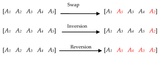
Figure 1.
Additional operators in the modified FA.
The proposed operators, in the beginning, create an arbitrary neighbour sol′ for the preliminary solution sol in the second group. Next, the value of fitness functions denoted by f(sol′) are calculated for all of them. In case f(sol′) has a better value compared to the f(sol) (the value of fitness function for the first group), sol′ is recognized as a new answer which means a potential solution and also is substituted with sol; in any other case, the prior best solution stays in the second group as potential solutions. Lastly, the newly acquired solutions combined with a potential solution that are already in the first group and FA will be run to find the optimal solutions. Figure 2 depicts the graphical representation of the modified FA.
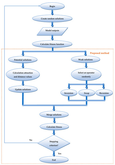
Figure 2.
Graphical representation of modified FA.
As can be seen in Figure 3, the proposed algorithm begins similarly to the standard FA by generating random solutions and calculating their fitness functions. Afterward, the modified FA divides the solutions in two groups namely potential and weak solutions. The modified FA calculates the attraction and distance values for the members in the potential solution group. Note that in the standard FA, the attraction and distance values are calculated for all generated solutions. It must be noted this excessive exploration slows down the convergence. More precisely, while in the first steps of the algorithm initialization, random solutions are generated and their fitness functions are calculated and these solutions are sorted based on their fitness values. Those solutions with very high values of fitness function (in the case of minimization problem) stand in the last positions in the sequence of potential solutions for the problem at hand. Consequently, calculating the attraction and distance values for these kinds of solutions is a waste of time, because it is scarce that these solutions are selected as the optimum answer for the problem. However, in the modified algorithm, to not limit the searching space, we categorized these solutions in weak solutions group, in case if they can help the algorithm to find optimum answers in the next iterations. Figure 3 presents the pseudo-code for the modified FA.
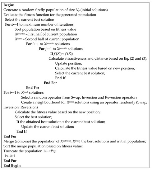
Figure 3.
Pseudo code for modified FA.
It should be noted that the proposed modified FA (depicted in Figure 3) differentiates from the classical FA by considering the additional operators (swap, reversion and inversion). In other word, the proposed modified FA sorts the population based on fitness value into two groups: potential and weak solution groups wherein classical FA, all population is considered in one group.
3. Results and Discussion
3.1. Problem Description
We consider a supply chain network problem to demonstrate the efficiency of the proposed modified FA. The investigated supply chain network problem in this study includes the decision associated with the distribution of multiple products that are produced by multiple manufacturers and distributed through multiple Distribution Centres (DCs) and Retailers. The schematic description of this problem is depicted in Figure 4.
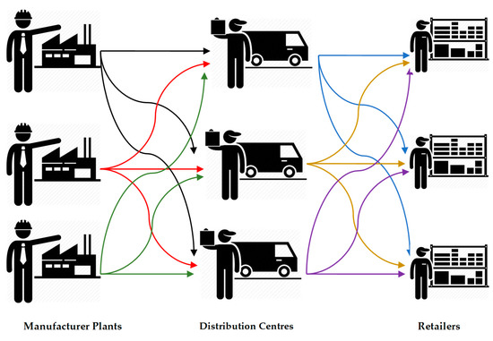
Figure 4.
The considered supply chain network.
In the following, the problem’s assumptions and model formulation are presented:
| i. Indices | |
| i | Index of manufacturing plants, i = 1, 2, …, I |
| j | Index of DCs, j = 1, 2, …, J |
| k | Index of retailers, k = 1, 2, …, K |
| p | Index of different kinds of items, p = 1, 2, …, P |
| t | Index of the planning period, t = 1, 2, …, T |
| I | Number of manufacturing plants |
| J | Number of DCs |
| K | Number of retailers |
| P | Number of items types |
| T | Number of periods |
| ii. Parameters | |
| Dkpt | Demand in retailer k for item p at the end of period t |
| Caipt | Supply capacity of manufacturing plant i for item p in period t |
| η jp | Holding cost per unit of item p at DC j in each period |
| Lij | Distance between manufacturer i and DC j |
| υp | Shipping cost per unit of item p along unit distance |
| L’jk | Distance (in kilometres) between DC j and retailer k |
| Ca’jt | Distribution capacity of DC j in period t |
| Vjt | Total storage (holding capacity) capacity of DC j during period t |
| η’kp | Holding cost per unit of item p at retailer k in each period |
| Skp | Backlog cost per unit of item p at retailer k |
| Ukt | Total holding capacity of retailer k during period t |
| iii. Decision variables | |
| Xijpt | Quantity of items p shipped from manufacturing plant i to DC j in period t |
| Ipjt | Inventory level of item p at DC j at the end of period t |
| Yjkpt | Quantity of item p shipped from DC j to retailer k during period t |
| Bpkt | Backlog amount of item p at retailer k in period t |
| Jpkt | Inventory of item p at retailer k at the end of period t |
• Objective Functions
Equation (5) represents the objective function that minimizes the total costs, consist of shipping costs from the plants to DCs () and from DCs to retailers (), costs of holding in both DCs () and retailers () and penalty charges regarding the quantity of backorders at retailers (). It should be noted that the shipping costs considered as proportional to the traveling distances.
• Constraints
i. Capacity Constraints
Constraints (6)–(8) are the capacity constraints and ensure the maximum allowable to be distributed or kept. More precisely, Constraint (6) takes into account that total items shipped from each manufacturing plant to all the DCs in every period do not exceed the supply capacity of that manufacturing plant. Constraint (7) denotes the capacity storage of DCs and Constraint (8) indicates the retailers’ storage capacity.
ii. Delivery Capacity Constraints
Constraint (9) shows the restrictions of delivery capacity for the DCs. This constraint ensures the number of products that are distributed from each DC, do not exceed the maximum capacity of each distributor.
iii. Flow Conservation Constraints
Constraints (10) and (11) formulate the flow conservation at DCs and retailers’ echelon respectively. These constraints mathematically ensure that the sum of the flow through a supply chain echelon toward another stage plus that stage’s supply and available inventories minus shortages, if any, equals the sum of the flow through a supply chain echelon directed away from that stage plus that node’s demand plus available inventories and minus shortages, if any.
iv. Non-negativity Constraint
Constraint (12) guarantees non-negativity values of the decision variables, since all the decision variables must be positive-integer numbers.
3.2. Design of Test Problems
In this research, to demonstrate the applicability and verification of the suggested model, several types problems consist of small, medium and large problems were taken into account in order to simulate different in close proximity to real-world situations. Each parameter’s value (in the considered cases) was produced on a random basis identified through uniform distribution in an interval between the lower and upper bounds of parameters. Table 2 presents the considered test problems.
Table 2.
Test problems size as suggested by [13].
It should be noted that problem size depends on the number of variables, constraints and the size of the search space (Talbi, 2009; Memari et al., 2016) and there is no obvious prior existing to categorize problems based on their sizes.
3.3. Experimental Results of Modified FAs
In order to demonstrate the efficiency of the proposed modified FA, the performances of the developed modified FA was compared to the classical FA. Four performance measures were used in this regard: (1) best fitness solution (Best_Sol), (2) CPU time, (3) relative percentage deviation (RPD) and (4) relative deviation index (RDI). RDI and the RPD are defined as (Talbi, 2009):
where Algsol is the value of the fitness function and Minsol and Maxsol denote the best and the worst solutions, respectively. It must be noted that the lower values of both RDI and RPD show the better efficiency of the considered algorithm. Note also that in this section, the best out of 5 solutions obtained were selected for comparison. Table 3 provides a comparison study of classical FA and modified FA.
Table 3.
Performances comparison of FA and modified FA.
As can be seen from the obtained results presented in Table 3, it is apparent the proposed modification makes the classical FA more efficient in terms of all considered performance metrics. The modified FA searches more in search space, therefore, it could obtain more feasible solutions. Closer inspection of the Table 3 reveals that the modified FA finds better solutions (in this case cheaper cost since the minimization problem is in run) for medium sizes problems (M1 and M2) by 1.69% and 1.51% respectively. The obtained solutions by modified FA (Best_Sol) are less than that of the classical FA by 0.41% on average for different sizes of problem. In addition, based on the required iterations to find the optimal solution, it can be seen that the modified algorithm can find the solution by 38.66% less iterations on average compared to the standard FA. Figure 5 confirms these claims.
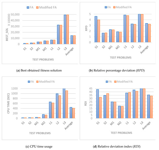
Figure 5.
Performances comparison of modified FA and FA.
The results, as shown in Table 3, indicate that regarding required computational time, the modified FA performs more efficient compared to classical with a significant reduction of computational time by 8.12% on average for the different size of problems. From the results depicted in Figure 4, it is apparent that the reduction of computational time between modified FA and classical FA for medium sizes problems are 11.31% and 13.87%. A possible explanation for this might be that the convergence of classical FA slows down because of too much exploration in standard FA. In fact, standard FA explores all possible solutions including weak solutions in a search space. This exploration leads to increase the required computational time.
As can be seen in the Figure 5, the best obtained solution function of both algorithms is almost identical. However, the modified algorithm found these values with less CPU time and fewer iterations. As a result, for more complicated and large sizes problems, the modified FA can perform more efficiently. In terms RPD metric while the values of metrics for both algorithms are close, however, for the smallest and the largest problem, the modified FA performs better than the standard FA. The values for RDI metric also show the modified FA in the smallest size problem S1 performs significantly better than the standard FA.
4. Conclusions
The search-based character of metaheuristics algorithms indicates that they might lose some of their speed when all searching parameters are needed. For experimental investigations and strategic decisions, this matter can be less of a concern. Nevertheless, for instant purposes like a real-life dynamic emergency vehicle routing problem in which every single second counted, extra moments of required time may make the approach improper to employ, even if a better solution can be found.
This study presented a new modification for the standard FA. A mixed integer linear programming model was developed for a supply chain network problem to demonstrate the efficiency of the proposed model. The findings showed that the proposed algorithm performs more efficient compared to classical FA. A common issue in running the standard FA is it usually stuck in stagnation or fall in premature convergence (fall into the local optimum) in searching space, especially for large size problems. This issue is connected with too much exploration and exploitation and inherent in the standard FA formulation. The proposed modification in this study resolves this issue by providing a balance between the exploitation and exploration in the standard FA.
The generalisability of these results is subject to certain limitations. For instance, the developed model was formulated as mixed integer linear programming. In order to develop the model further, care should be taken for nonlinear models. Nonlinear behaviour of parameters and variables might also result in different findings.
The obtained results of implementing metaheuristics approaches are very sensitive to their parameters. Consequently, a little change in their parameters may influence the quality of the obtained solutions. As a result, a fine-tuning procedure for the parameters is needed to find better solutions. However, parameter tuning has almost neglected in all studies in the area under investigation by this research and the previous studies in the area generally have found metaheuristics parameters setting using a trial and error procedure. A further study could assess the effects of parameters’ setting on the performance of the proposed algorithm.
Author Contributions
Methodology, A.M.; software, A.M.; validation, A.R.A.R., R.A. and M.R.A.J.; formal analysis, A.M.; investigation, A.R.A.R.; resources, M.R.A.J.; data curation, A.M.; writing—original draft preparation, A.M.; writing—review and editing, A.M.; visualization, M.R.A.J.; supervision, R.A.; funding acquisition.
Funding
This research was funded by Universiti Teknologi Malaysia (UTM) and Ministry of Higher Education (MOHE) Malaysia under Professional Development Research University (PDRU) grant Vot Q.J130000.21A2.04E15, for the project “An optimization model of oil-palm biomass supply chain for sustainable power generation in Malaysia” Vot Q.K130000.2601.15J23.
Conflicts of Interest
The authors declare no conflict of interest. The funders had no role in the design of the study; in the collection, analyses or interpretation of data; in the writing of the manuscript or in the decision to publish the results.
References
- Yang, X.S. Firefly algorithm. In Nature-Inspired Metaheuristic Algorithms; Yang, X.-S., Ed.; Wiley Online Library: Hoboken, NJ, USA, 2008; pp. 79–90. [Google Scholar]
- Talbi, E.-G. Metaheuristics: From Design to Implementation; John Wiley & Sons: Hoboken, NJ, USA, 2009; Volume 74. [Google Scholar]
- Memari, A.; Ahmad, R.; Rahim, A.R.A. Metaheuristic Algorithms: Guidelines for Implementation. J. Soft Comput. Decis. Support Syst. 2017, 4, 1–6. [Google Scholar]
- Kirkpatrick, S.; Gelatt, C.D.; Vecchi, M.P. Optimization by simulated annealing. Science 1983, 220, 671–680. [Google Scholar] [CrossRef] [PubMed]
- Fister, I.; Yang, X.-S.; Fister, D. Firefly algorithm: A brief review of the expanding literature. In Cuckoo Search and Firefly Algorithm; Springer: New York, NY, USA, 2014; pp. 347–360. [Google Scholar]
- Fister, I.; Fister, I., Jr.; Yang, X.-S.; Brest, J. A comprehensive review of firefly algorithms. Swarm Evol. Comput. 2013, 13, 34–46. [Google Scholar] [CrossRef]
- Husselmann, A.V.; Hawick, K. Parallel parametric optimisation with firefly algorithms on graphical processing units. In Proceedings of the 2012 International Conference on Genetic and Evolutionary Methods (GEM’12), Las Vegas, NV, USA, 16–19 July 2012; pp. 77–83. [Google Scholar]
- Subutic, M.; Tuba, M.; Stanarevic, N. Parallelization of the firefly algorithm for unconstrained optimization problems. Latest Adv. Inf. Sci. Appl. 2012, 22, 264–269. [Google Scholar]
- Eswari, R.; Nickolas, S. Modified multi-objective firefly algorithm for task scheduling problem on heterogeneous systems. Int. J. Bio-Inspired Comput. 2016, 8, 379–393. [Google Scholar] [CrossRef]
- Tilahun, S.L.; Ong, H.C. Modified Firefly Algorithm. J. Appl. Math. 2012, 2012, 12. [Google Scholar] [CrossRef]
- Abdullah, A.; Deris, S.; Anwar, S.; Arjunan, S.N. An evolutionary firefly algorithm for the estimation of nonlinear biological model parameters. PLoS ONE 2013, 8, e56310. [Google Scholar] [CrossRef] [PubMed]
- Abdullah, A.; Deris, S.; Mohamad, M.S.; Anwar, S. An Improved Swarm Optimization for Parameter Estimation and Biological Model Selection. PLoS ONE 2013, 8, e61258. [Google Scholar] [CrossRef]
- Memari, A.; Rahim, A.R.A.; Absi, N.; Ahmad, R.; Hassan, A. Carbon-capped distribution planning: A JIT perspective. Comput. Ind. Eng. 2016, 97, 111–127. [Google Scholar] [CrossRef]
- Ji-jun, Y. Optimal design for scale-based product family based on multi-objective firefly algorithm. Comput. Integr. Manuf. Syst. 2012, 8, 020. [Google Scholar]
- Yang, X.-S. Efficiency analysis of swarm intelligence and randomization techniques. J. Comput. Theor. Nanosci. 2012, 9, 189–198. [Google Scholar] [CrossRef]
- Yang, X.-S. Firefly algorithm, Levy flights and global optimization. In Research and Development in Intelligent Systems XXVI; Springer: New York, NY, USA, 2010; pp. 209–218. [Google Scholar]
- Chandrasekaran, K.; Simon, S.P. Network and reliability constrained unit commitment problem using binary real coded firefly algorithm. Int. J. Electr. Power Energy Syst. 2012, 43, 921–932. [Google Scholar] [CrossRef]
- Falcon, R.; Almeida, M.; Nayak, A. Fault identification with binary adaptive fireflies in parallel and distributed systems. In Proceedings of the 2011 IEEE Congress on Evolutionary Computation (CEC), New Orleans, LA, USA, 5–8 June 2011; pp. 1359–1366. [Google Scholar]
- Palit, S.; Sinha, S.N.; Molla, M.A.; Khanra, A.; Kule, M. A cryptanalytic attack on the knapsack cryptosystem using binary Firefly algorithm. In Proceedings of the 2011 2nd International Conference on Computer and Communication Technology (ICCCT), Allahabad, India, 15–17 September 2011; pp. 428–432. [Google Scholar]
- Xu, G.; Wu, S.; Tan, Y. Island Partition of Distribution System with Distributed Generators Considering Protection of Vulnerable Nodes. Appl. Sci. 2017, 7, 1057. [Google Scholar] [CrossRef]
- Farahani, S.M.; Abshouri, A.; Nasiri, B.; Meybodi, M. A Gaussian firefly algorithm. Int. J. Mach. Learn. Comput. 2011, 1, 448–453. [Google Scholar] [CrossRef]
- Bottani, E.; Centobelli, P.; Cerchione, R.; Gaudio, L.; Murino, T. Solving machine loading problem of flexible manufacturing systems using a modified discrete firefly algorithm. Int. J. Ind. Eng. Comput. 2017, 8, 363–372. [Google Scholar] [CrossRef]
- Coelho, L.D.S.; de Andrade Bernert, D.L.; Mariani, V.C. A chaotic firefly algorithm applied to reliability-redundancy optimization. In Proceedings of the 2011 IEEE Congress on Evolutionary Computation (CEC), New Orleans, LA, USA, 5–8 June 2011; pp. 517–521. [Google Scholar]
- Gandomi, A.; Yang, X.-S.; Talatahari, S.; Alavi, A. Firefly algorithm with chaos. Commun. Nonlinear Sci. Numer. Simul. 2013, 18, 89–98. [Google Scholar] [CrossRef]
© 2018 by the authors. Licensee MDPI, Basel, Switzerland. This article is an open access article distributed under the terms and conditions of the Creative Commons Attribution (CC BY) license (http://creativecommons.org/licenses/by/4.0/).