Evolutionary Algorithm-Based Friction Feedforward Compensation for a Pneumatic Rotary Actuator Servo System


Abstract
1. Introduction
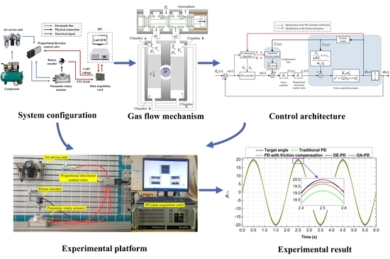
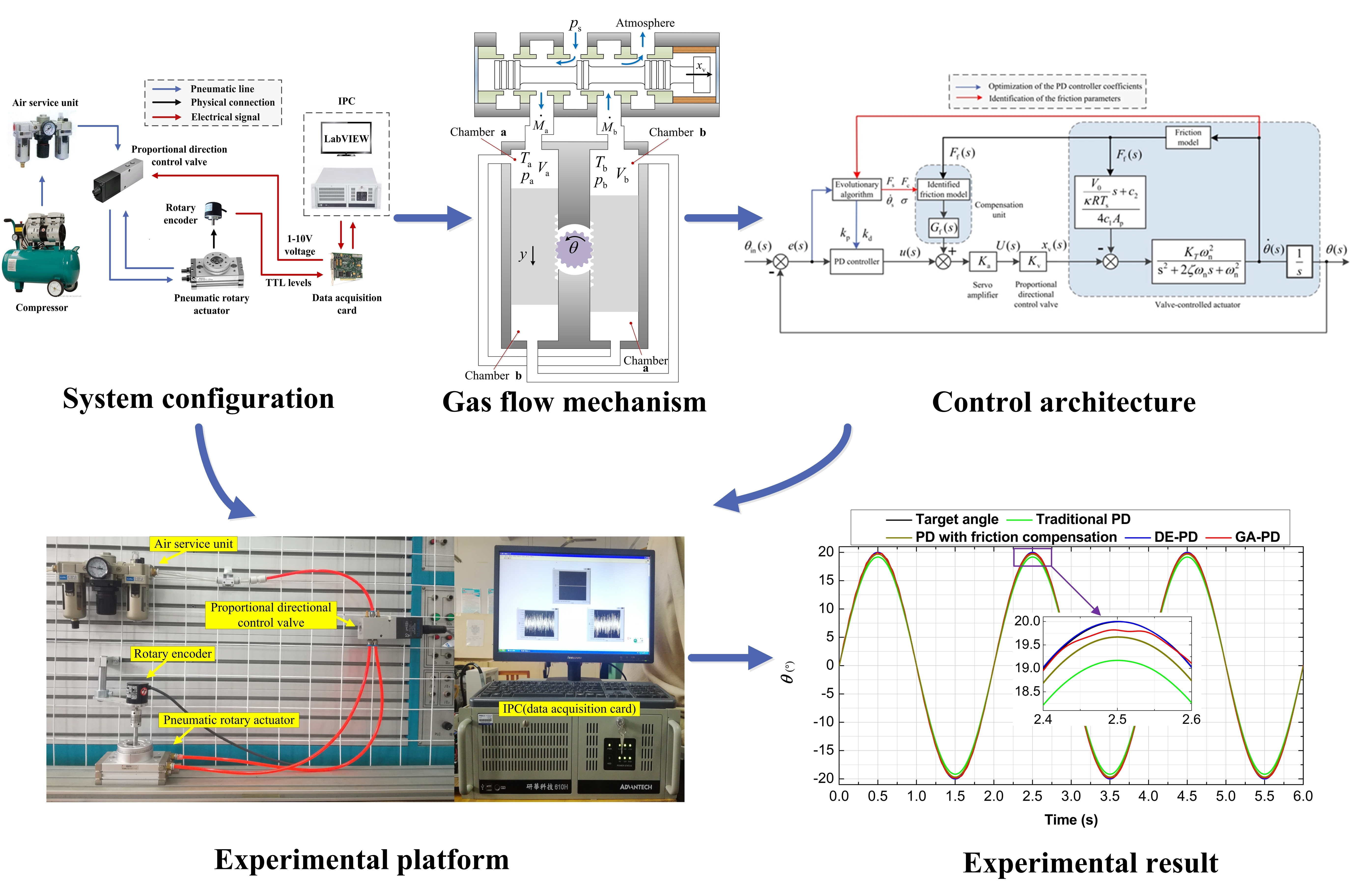
2. System Configuration
3. System Modeling
- (1)
- The working medium is ideal gas, which follows the ideal gas law.
- (2)
- Supply pressure and supply temperature are constant, and the parameter of each point in the chamber is equal at each instant.
- (3)
- There is no leakage between the valve-controlled actuator system and the outside and between the two chambers.
- (4)
- The flow state of the gas flowing through the orifice is an isentropic adiabatic process.
- (5)
- The change of each parameter in the dynamic process is only a small amount (small disturbance hypothesis).
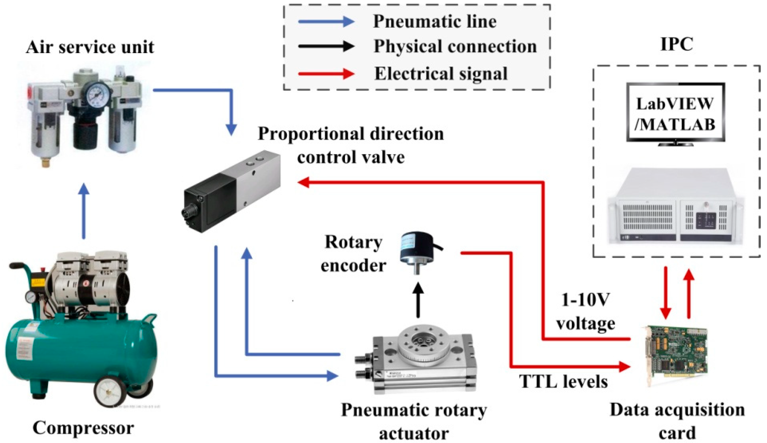
3.1. Orifice Equation of the Mass Flow Rate
3.2. Continuity Equation of the Mass Flow Rate
3.3. Dynamic Equation of the Actuator
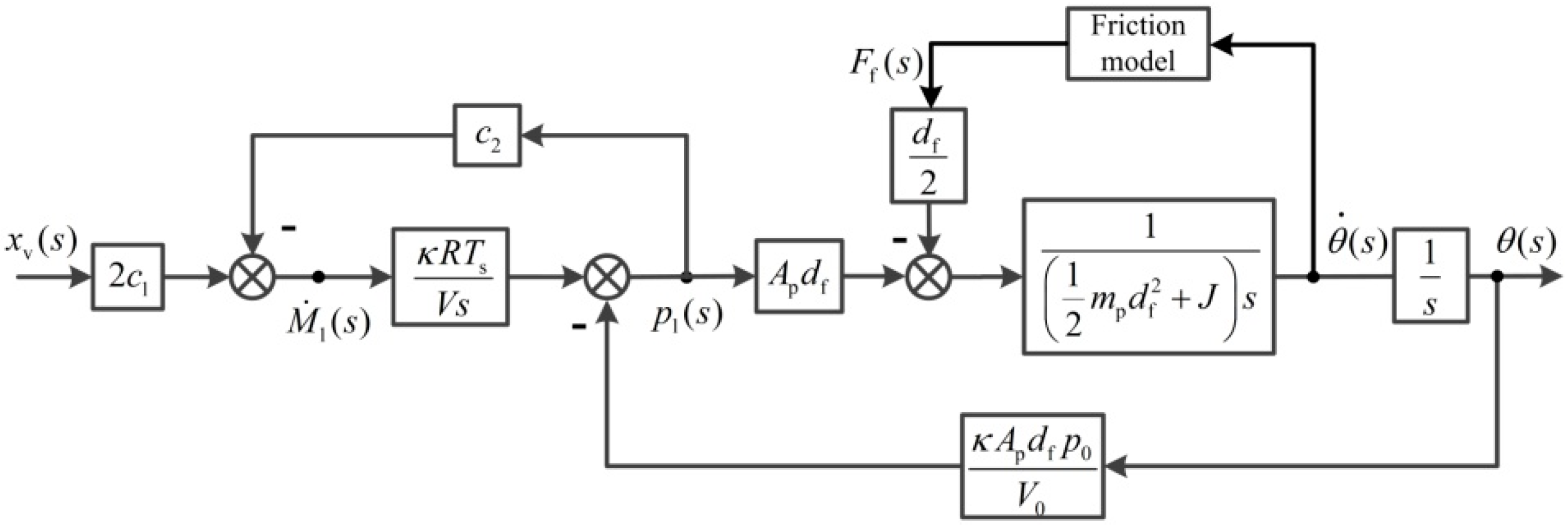
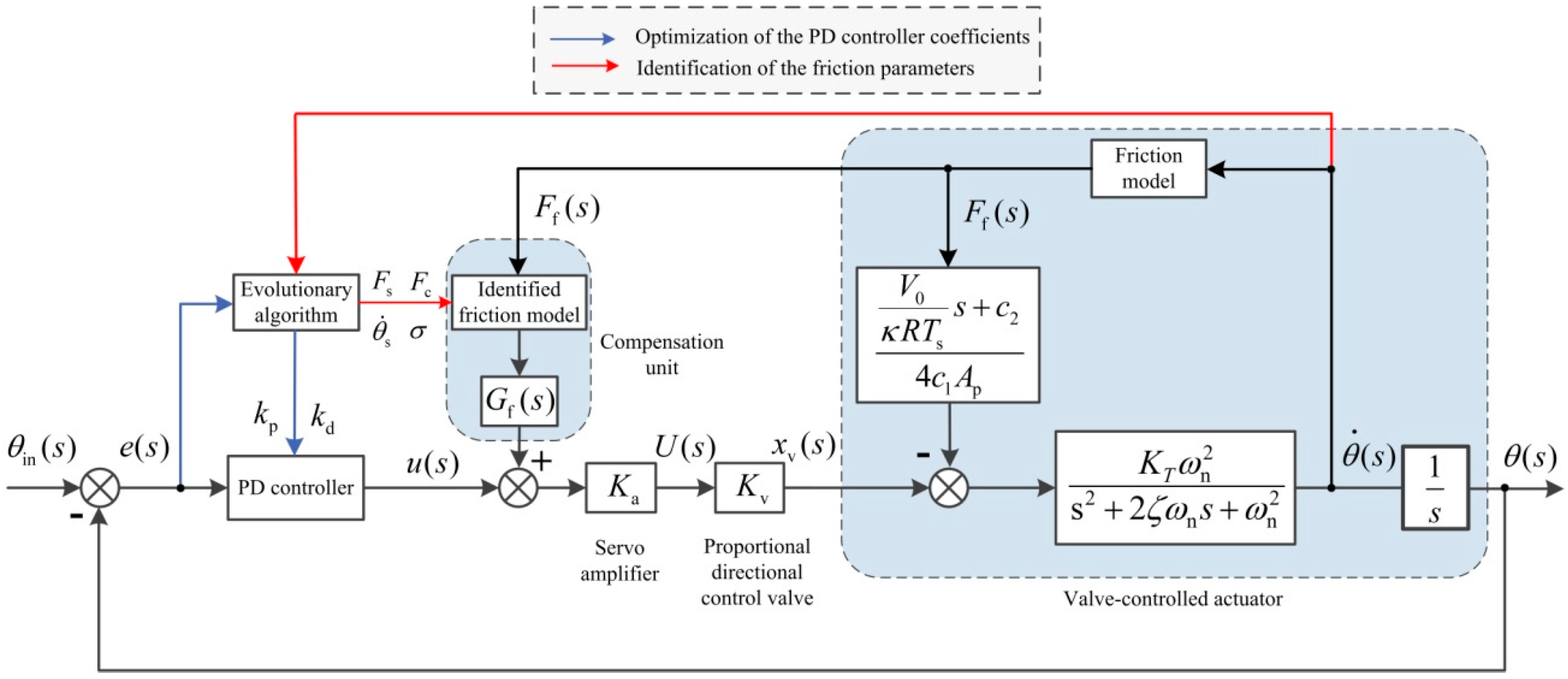
3.4. Block Diagram and Transfer Function of the Valve-Controlled Actuator System
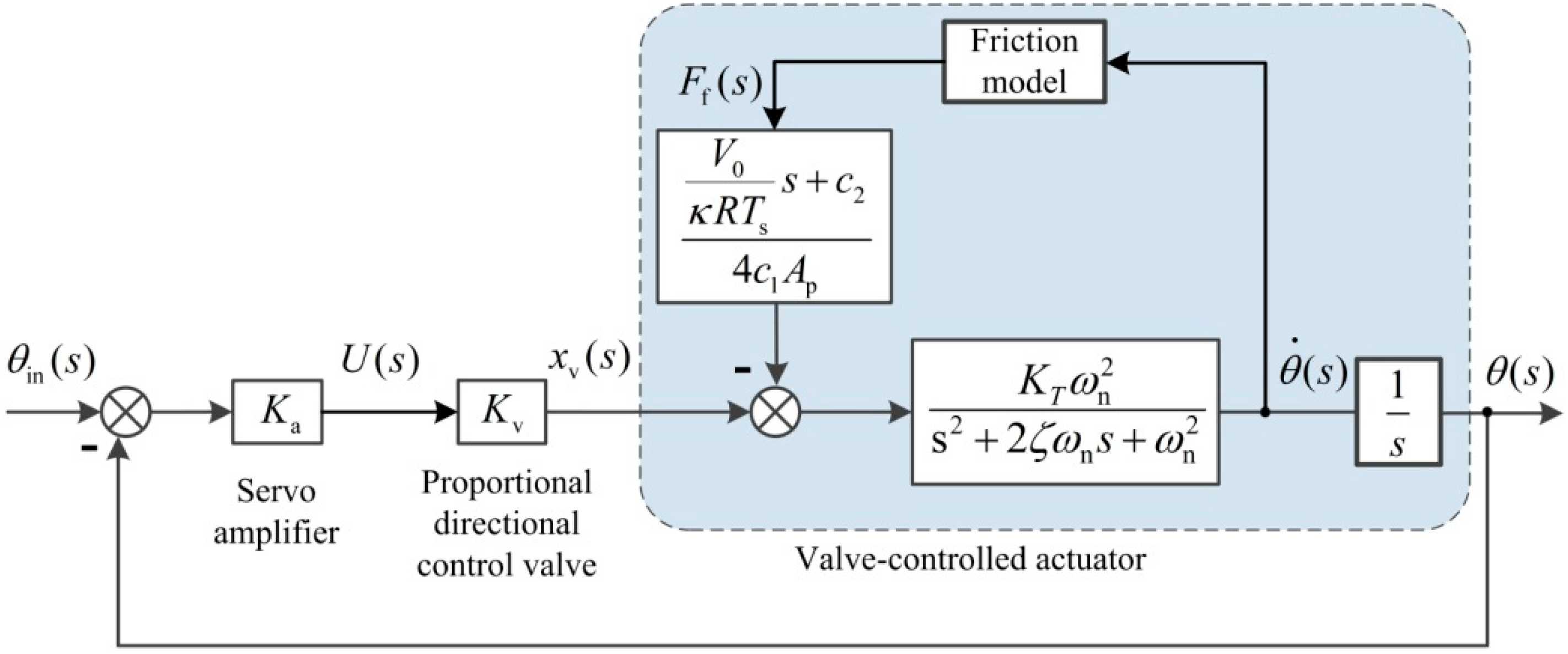
3.5. The Transfer Function of the Pneumatic Rotary Actuator Servo System
4. Control Design
4.1. PD Controller and Compensation Unit
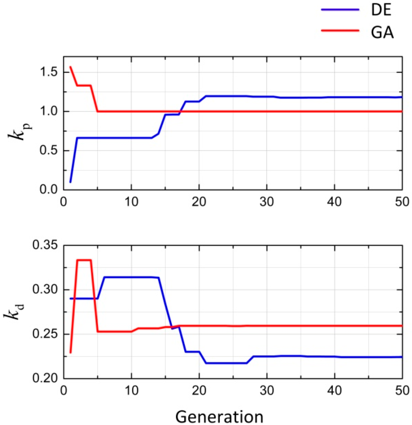
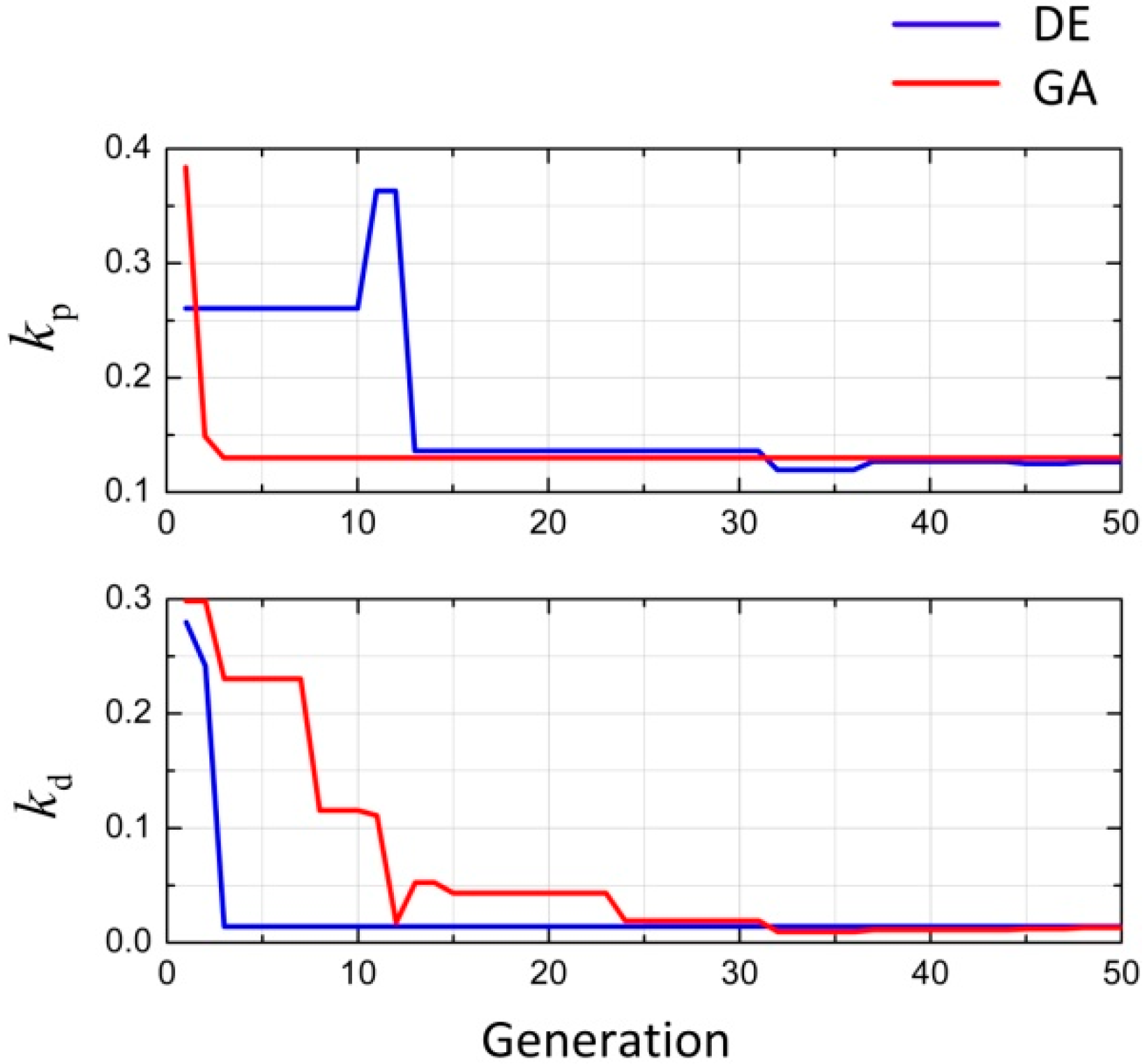
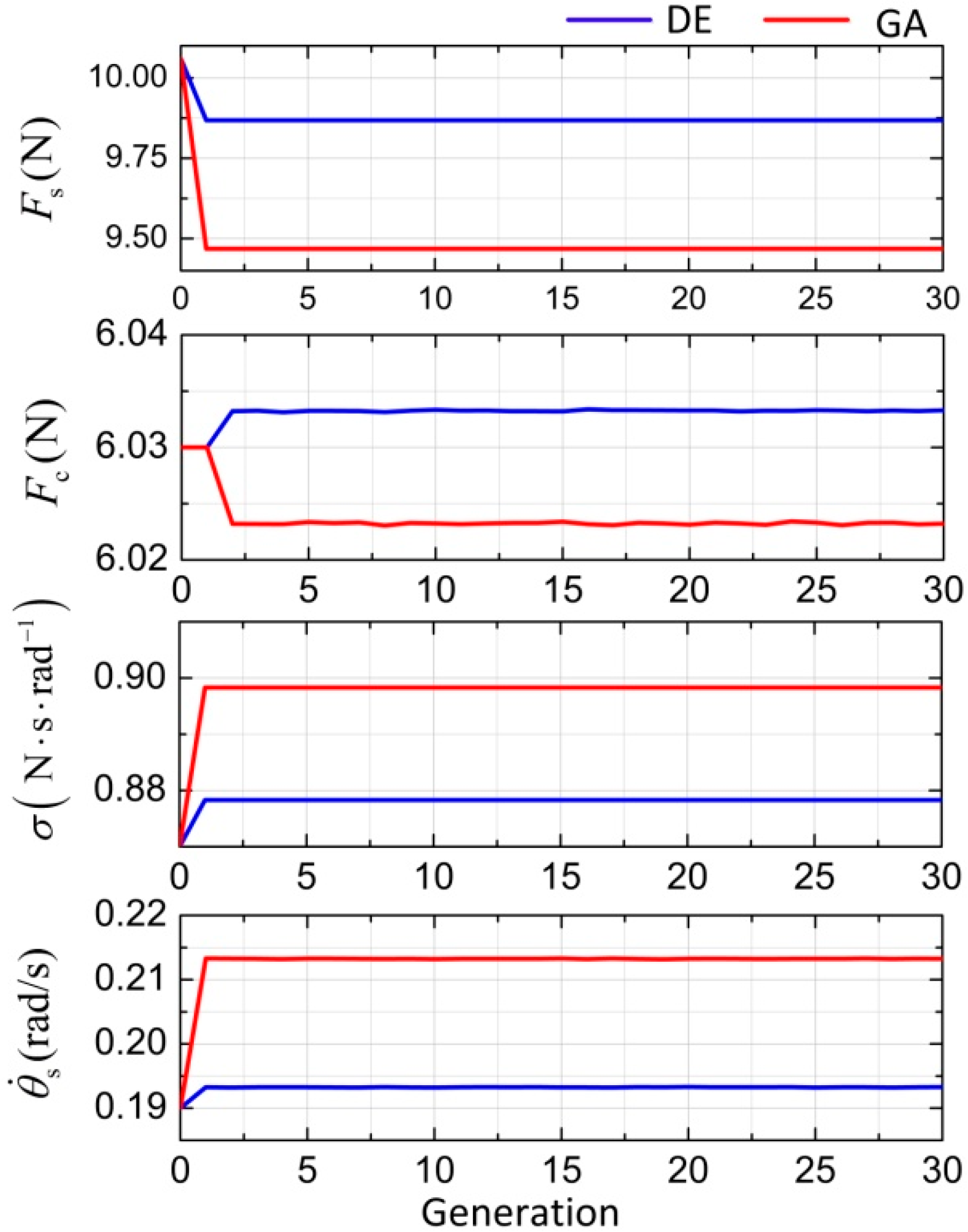
4.2. Evolutionary Algorithms
4.2.1. Differential Evolution Algorithm
- Step 1: Generation of initial population
- Step 2: Mutation
- Step 3: Crossover
- Step 4: Selection
- Step 5: Iteration and end condition
4.2.2. Genetic Algorithm
- Step 1: Coding scheme
- Step 2: Initial population formation
- Step 3: Fitness function design
- Step 4: Evolutionary process
- Selection: Produce a new generation population by selecting operation.
- Crossover: Implement crossover operation with the cross probability .
- Mutation: Implement mutation operation with the mutation probability .
- Step 5: Iteration and end condition
5. Experimental Results and Analysis
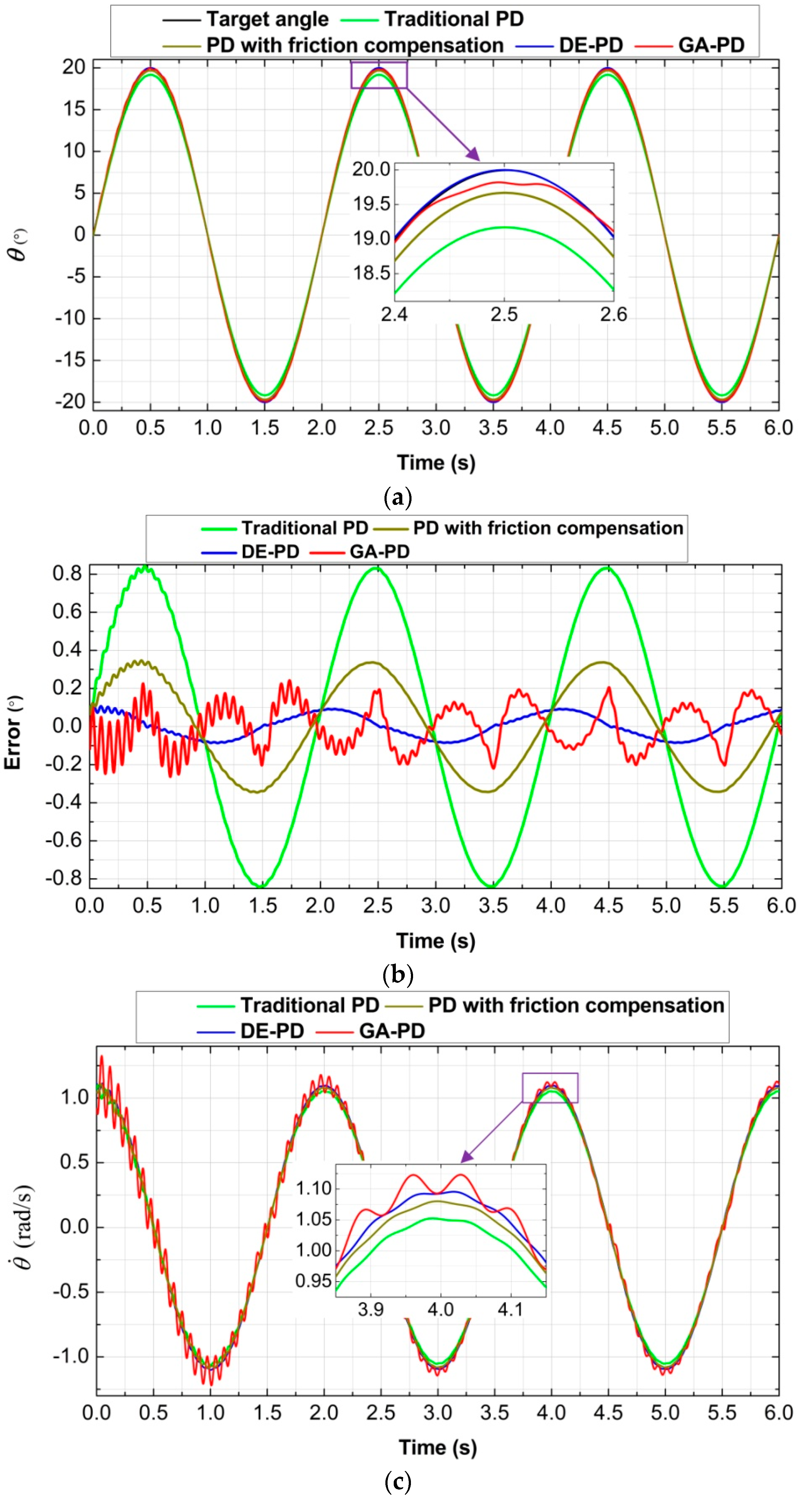
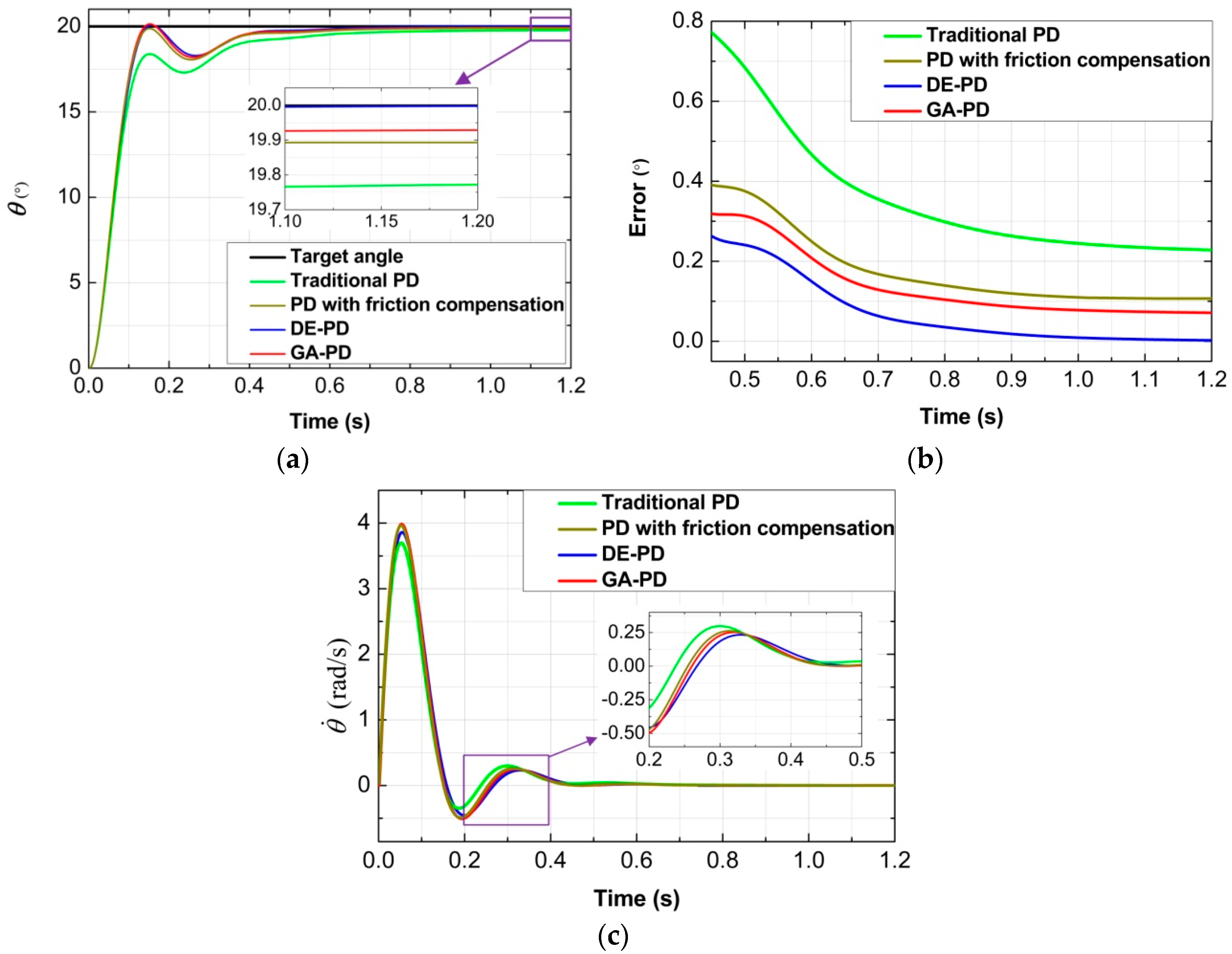
5.1. Position Tracking Experiment
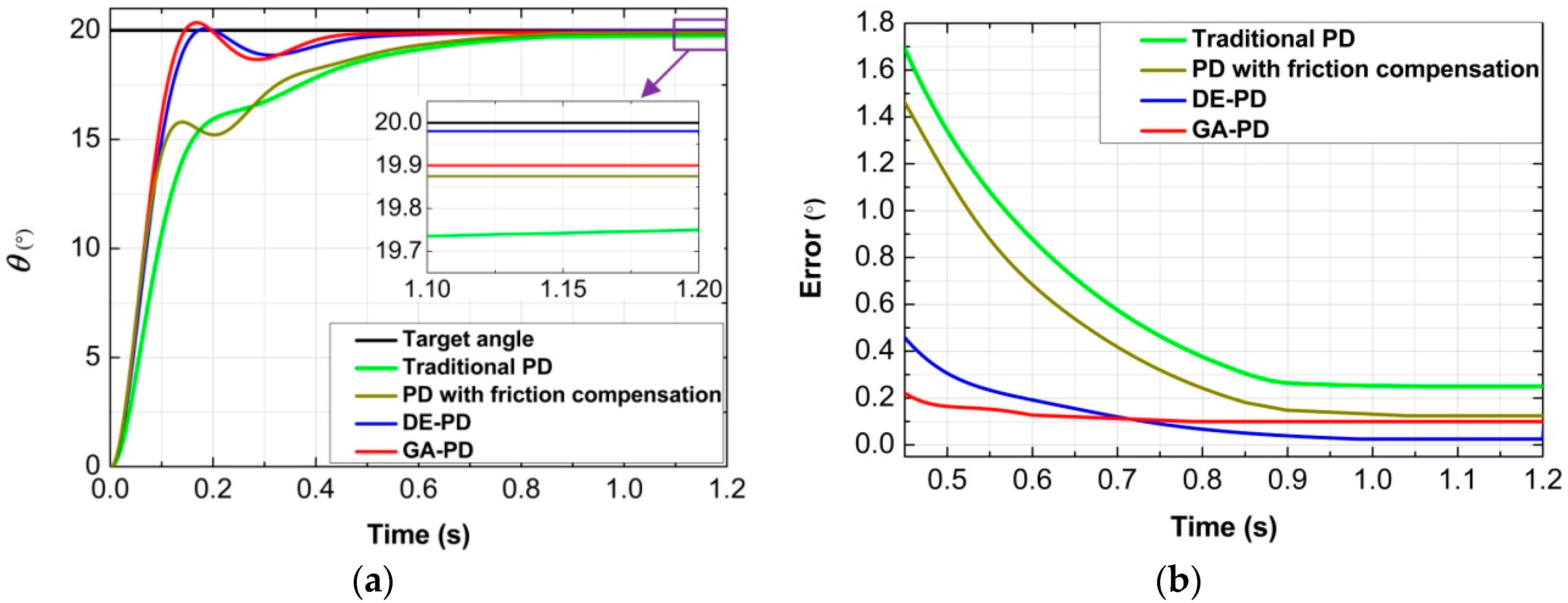
5.2. Positioning Experiment
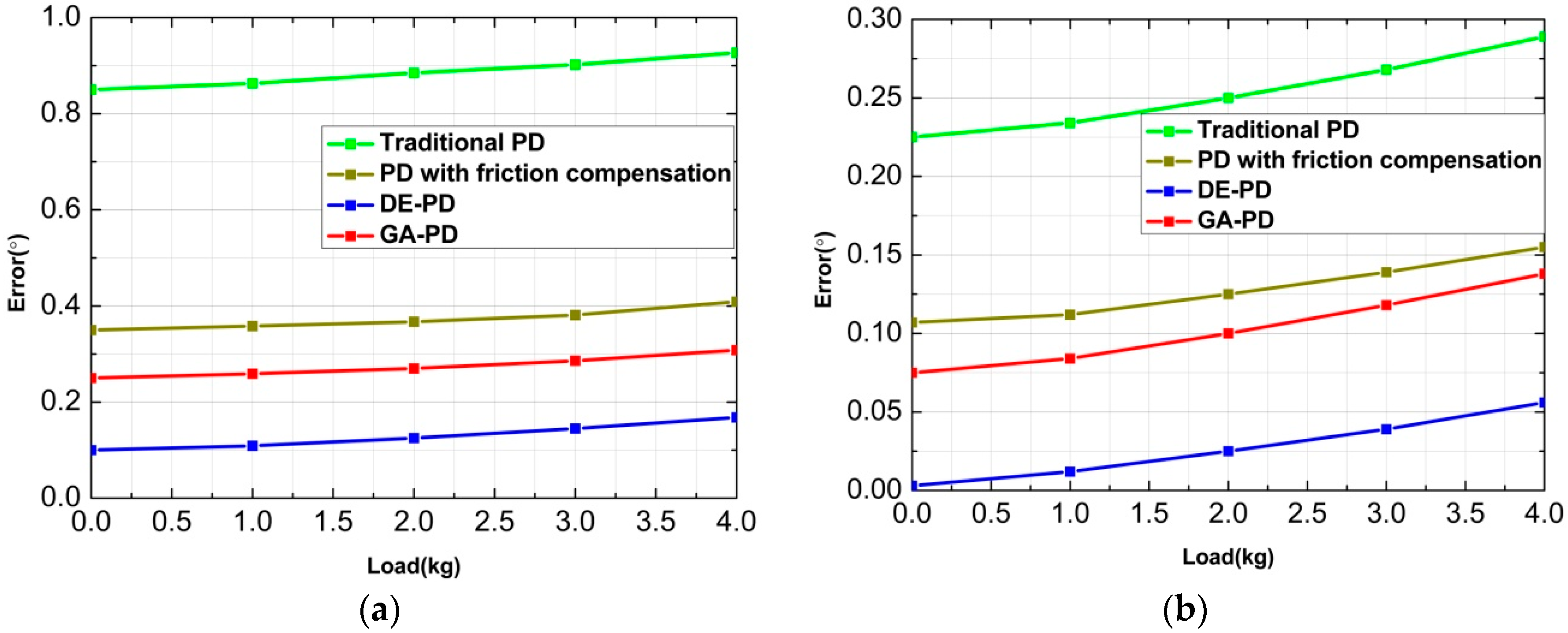
5.3. Stability Experiment with Load
6. Conclusions
- (1)
- The PD control with friction feedforward compensation without evolutionary algorithm tuning can reduce the system error to a certain extent. However, since the controller parameters and friction parameters were not optimized, the error values were still relatively large.
- (2)
- The friction feedforward compensation based on evolutionary algorithm greatly improved the position tracking performance for the sinusoidal signal, and the DE-based case had better control accuracy and smaller velocity fluctuations.
- (3)
- The friction feedforward compensation based on evolutionary algorithm greatly improved the positioning performance when the input angle was a constant, and the DE-based case achieved higher accuracy.
- (4)
- Although the existence of the load affected the tracking and positioning effects, the system with the evolutionary algorithm-based friction feedforward compensation still maintained high accuracy and strong stability.
Author Contributions
Funding
Acknowledgments
Conflicts of Interest
References
- Ning, F.; Shi, Y.; Cai, M.; Wang, Y.; Xu, W. Research Progress of Related Technologies of Electric-Pneumatic Pressure Proportional Valves. Appl. Sci. 2017, 7, 1074. [Google Scholar] [CrossRef]
- Shi, Y.; Wang, Y.; Cai, M.; Zhang, B.; Zhu, J. An aviation oxygen supply system based on a mechanical ventilation model. Chin. J. Aeronaut. 2018, 31, 197–204. [Google Scholar] [CrossRef]
- Niu, J.; Shi, Y.; Cao, Z.; Cai, M.; Chen, W.; Zhu, J.; Xu, W. Study on air flow dynamic characteristic of mechanical ventilation of a lung simulator. Sci. Chin. Technol. Sci. 2017, 60, 243–250. [Google Scholar] [CrossRef]
- Zhang, Y.M.; Cai, M.L. Overall life cycle comprehensive assessment of pneumatic and electric actuator. Chin. J. Mech. Eng. 2014, 27, 584–594. [Google Scholar] [CrossRef]
- Nie, S.; Liu, X.; Yin, F.; Ji, H.; Zhang, J. Development of a High-Pressure Pneumatic On/Off Valve with High Transient Performances Direct-Driven by Voice Coil Motor. Appl. Sci. 2018, 8, 611. [Google Scholar] [CrossRef]
- Niu, J.; Shi, Y.; Cai, M.; Cao, Z.; Wang, D.; Zhang, Z.; Zhang, X.D. Detection of Sputum by Interpreting the Time-frequency Distribution of Respiratory Sound Signal Using Image Processing Techniques. Bioinformatics 2017, 34, 820–827. [Google Scholar] [CrossRef] [PubMed]
- Shi, Y.; Zhang, B.; Cai, M.; Xu, W. Coupling Effect of Double Lungs on a VCV Ventilator with Automatic Secretion Clearance Function. IEEE/ACM Trans. Comput. Biol. Bioinform. 2017. [Google Scholar] [CrossRef] [PubMed]
- Shi, Y.; Hao, L.; Cai, M.; Wang, Y.; Yao, J.; Li, R.; Feng, Q.; Li, Y. High-precision diameter detector and three-dimensional reconstruction method for oil and gas pipelines. J. Petrol. Sci. Eng. 2018, 165, 842–849. [Google Scholar] [CrossRef]
- Saravanakumar, D.; Mohan, B.; Muthuramalingam, T. A review on recent research trends in servo pneumatic positioning systems. Precis. Eng. 2017, 49, 481–492. [Google Scholar] [CrossRef]
- Kim, D.-S.; Lee, W.-H. Development of the Pneumatic Rotary Actuator for Marine Winch. J. Korean Soc. Mar. Eng. 2004, 28, 354–360. [Google Scholar]
- Chen, S.Y.; Gong, S.S. Speed tracking control of pneumatic motor servo systems using observation-based adaptive dynamic sliding-mode control. Mech. Syst. Signal Process. 2017, 94, 111–128. [Google Scholar] [CrossRef]
- Ren, S.; Cai, M.; Shi, Y.; Xu, W.; Zhang, X.D. Influence of bronchial diameter change on the airflow dynamics based on a pressure-controlled ventilation system. Int. J. Numer. Methods Biomed. Eng. 2017, 34, e2929. [Google Scholar] [CrossRef] [PubMed]
- Valdiero, A.C.; Ritter, C.S.; Rios, C.F.; Rafikov, M. Nonlinear mathematical modeling in pneumatic servo position applications. Math. Probl. Eng. 2011, 2011, 472903. [Google Scholar] [CrossRef]
- Armstrong-Hélouvry, B.; Dupont, P.; Wit, C.C.D. A survey of models, analysis tools and compensation methods for the control of machines with friction. Automatica 1994, 30, 1083–1138. [Google Scholar] [CrossRef]
- Rad, C.-R.; Hancu, O. An improved nonlinear modelling and identification methodology of a servo-pneumatic actuating system with complex internal design for high-accuracy motion control applications. Simul. Model. Pract. Theory 2017, 75, 29–47. [Google Scholar] [CrossRef]
- Gao, X.; Feng, Z.J. Design study of an adaptive Fuzzy-PD controller for pneumatic servo system. Control Eng. Pract. 2005, 13, 55–65. [Google Scholar] [CrossRef]
- Meng, D.; Tao, G.; Liu, H.; Zhu, X. Adaptive robust motion trajectory tracking control of pneumatic cylinders with lugre model-based friction compensation. Chin. J. Mech. Eng. 2014, 27, 802–815. [Google Scholar] [CrossRef]
- Sobczyk, M.R.; Gervini, V.I.; Perondi, E.A.; Cunha, M.A.B. A Continuous Version of the LuGre Friction Model Applied to the Adaptive Control of a Pneumatic Servo System. J. Frankl. Inst. 2016, 353, 3021–3039. [Google Scholar] [CrossRef]
- Guenther, R.; Perondi, E.A.; Depieri, E.R.; Valdiero, A.C. Cascade controlled pneumatic positioning system with LuGre model based friction compensation. J. Braz. Soc. Mech. Sci. Eng. 2006, 28, 48–57. [Google Scholar] [CrossRef]
- Xu, J.; Qiao, M.; Wang, W.; Miao, Y. Fuzzy PID Control for Ac Servo System Based on Stribeck Friction Model; Strategic Technology (IFOST): Ulsan, South Korea, 2011; pp. 706–711. [Google Scholar]
- Márton, L.; Fodor, S.; Sepehri, N. A practical method for friction identification in hydraulic actuators. Mechatronics 2011, 21, 350–356. [Google Scholar] [CrossRef]
- Castro, R.D.; Todeschini, F.; Rui, E.A.; Savaresi, S.M.; Corno, M.; Freitas, D. Adaptive-robust friction compensation in a hybrid brake-by-wire actuator. Proc. Inst. Mech. Eng. Part I J. Syst. Eng. 2014, 228, 769–786. [Google Scholar] [CrossRef]
- Zhang, Y.; Li, K.; Wei, S.; Wang, G. Pneumatic Rotary Actuator Position Servo System Based on ADE-PD Control. Appl. Sci. 2018, 8, 406. [Google Scholar] [CrossRef]
- Dangor, M.; Dahunsi, O.A.; Pedro, J.O.; Ali, M.M. Evolutionary algorithm-based PID controller tuning for nonlinear quarter-car electrohydraulic vehicle suspensions. Nonlinear Dynam. 2012, 78, 2795–2810. [Google Scholar] [CrossRef]
- Pedro, J.O.; Dangor, M.; Dahunsi, O.A.; Ali, M.M. Differential Evolution-Based PID Control of Nonlinear Full-Car Electrohydraulic Suspensions. Math. Probl. Eng. 2013, 2013, 532–548. [Google Scholar] [CrossRef]
- Jiao, Z.; Qu, B.; Xu, B. Application of Genetic Algorithm to Friction Compensation in Direct Current Servo Systems. J. Xian Jiaotong Univ. 2007, 8, 017. [Google Scholar]
- Jiao, Z.; Qu, B.; Xu, B. DC servo motor friction compensation using a genetic algorithm. J. Tsinghua Univ. 2007, S2. [Google Scholar]
- Shi, Y.; Cai, M. Working characteristics of two kinds of air-driven boosters. Energy Convers. Manag. 2011, 52, 3399–3407. [Google Scholar] [CrossRef]
- Shi, Y.; Wu, T.; Cai, M.; Wang, Y.; Xu, W. Energy conversion characteristics of a hydropneumatic transformer in a sustainable-energy vehicle. Appl. Energy 2016, 171, 77–85. [Google Scholar] [CrossRef]
- Shi, Y.; Wang, Y.; Liang, H.; Cai, M. Power characteristics of a new kind of air-powered vehicle. Int. J. Energy Res. 2016, 40, 1112–1121. [Google Scholar] [CrossRef]
- Shi, Y.; Zhang, B.; Cai, M.; Zhang, X.D. Numerical simulation of volume-controlled mechanical ventilated respiratory system with 2 different lungs. Int. J. Numer. Methods Biomed. Eng. 2017, 33, e2852. [Google Scholar] [CrossRef] [PubMed]
- Ren, S.; Shi, Y.; Cai, M.; Xu, W. Influence of secretion on airflow dynamics of mechanical ventilated respiratory system. IEEE/ACM Trans. Comput. Biol. Bioinform. 2018, PP, 1. [Google Scholar] [CrossRef] [PubMed]
- Peter, B. Pneumatic Drives System Design, Modeling and Control; Springer: Berlin/Heidelberg, Germany, 2007. [Google Scholar]
- Sanville, F. A new method of specifying the flow capacity of pneumatic fluid power valves. Hydraul. Pneum. Power 1971, 17, 120–126. [Google Scholar]
- Qiu, Z.C.; Shi, M.L.; Wang, B.; Xie, Z.W. Genetic algorithm based active vibration control for a moving flexible smart beam driven by a pneumatic rod cylinder. J. Sound Vib. 2012, 331, 2233–2256. [Google Scholar] [CrossRef]
- Andromeda, T.; Yahya, A.; Samion, S.; Baharom, A.; Hashim, N.L. Differential evolution for optimization of PID gain in Electrical Discharge Machining control system. Trans. Can. Soc. Mech. Eng. 2013, 37, 293–301. [Google Scholar] [CrossRef]
- Operation Manual of Pneumatic Rotary Actuator MSQ. Available online: http://www.smcworld.com/assets/manual/en-jp/files/MSQ-E.pdf (accessed on 2 September 2018).


| Component | Model | Parameters |
|---|---|---|
| Compressor | PANDA 750-30L | Maximum supply pressure: 0.8 MPa |
| Air service unit | AC3000-03 | Maximum working pressure: 1.0 MPa |
| Proportional directional control valve | FESTO MPYE-5-M5-010-B | 5/3-way valve, 0~10 V driving voltage |
| Pneumatic rotary actuator | SMC MSQA30A | Bore: 30 mm; stroke: 190° |
| Rotary encoder | E58S10 | Resolution: 36000 P/R |
| Data acquisition card | NI PCI-6229 | 32-bit counter; −10~10 V voltage output |
| IPC | IPC-610H | Standard configuration |
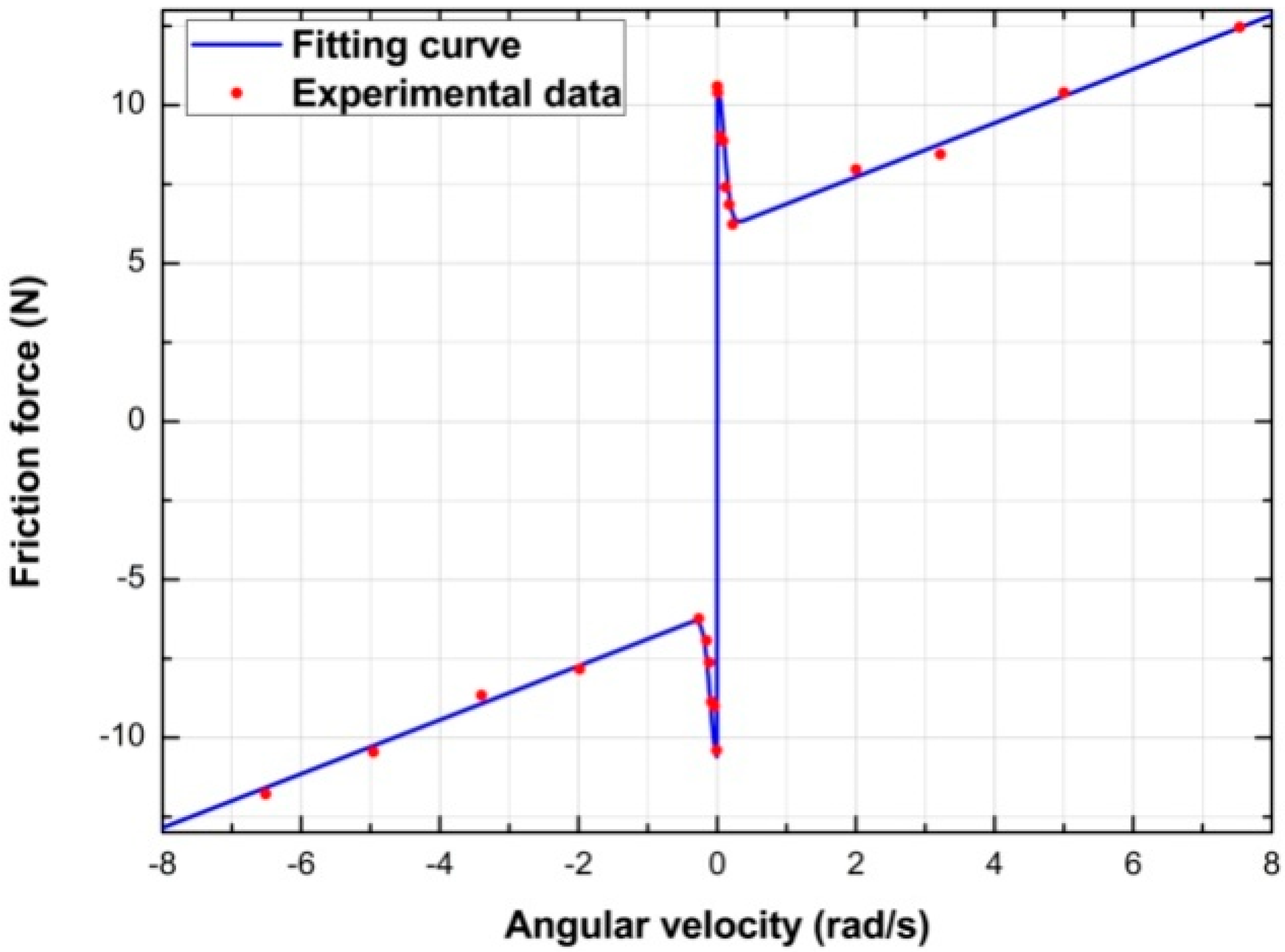
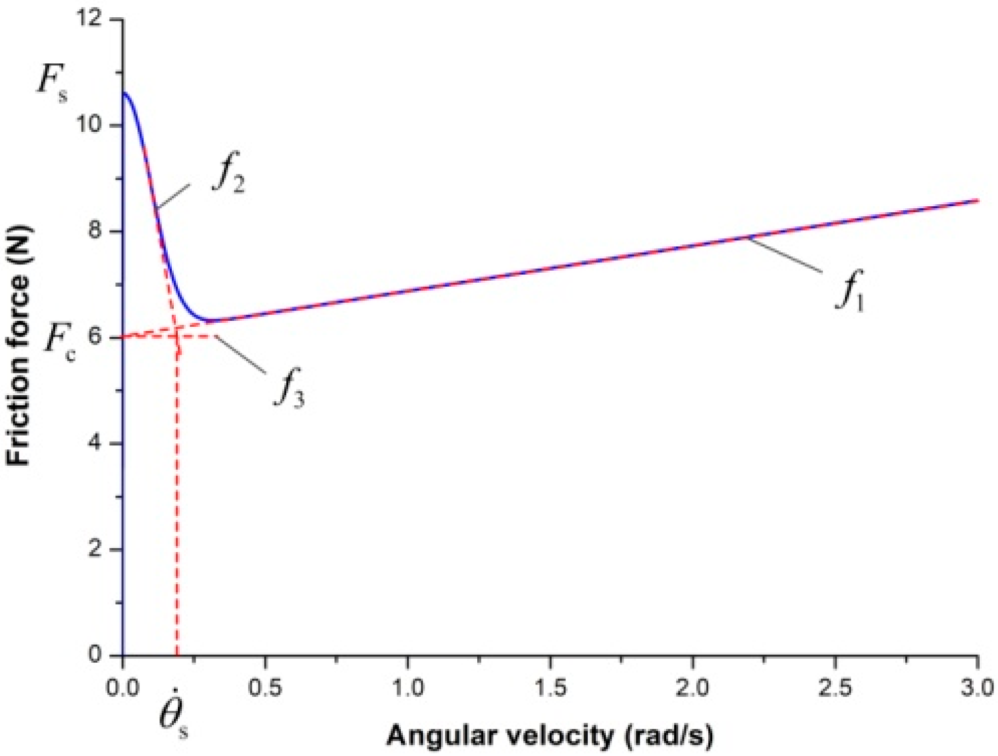
| Friction Parameter | Value |
|---|---|
| 10.60 (N) | |
| 6.03 (N) | |
| 0.19 (rad/s) | |
| 0.87 (N·s·rad−1) |
| Parameter | Value |
|---|---|
| 3.4636 × 10⁻⁴ [m2] | |
| 0.68 | |
| 0.21 | |
| 0.014 [m] | |
| 1.678 × 10⁻³ [kg·m2] | |
| 1.4 | |
| 2.1 [kg] | |
| 1.013 × 10⁵ [Pa] | |
| 287 [J/(kg·K)] | |
| 293 [K] | |
| 1.6767 × 10⁻⁵ [m3] | |
| 3.1415 × 10⁻² [m] |
© 2018 by the authors. Licensee MDPI, Basel, Switzerland. This article is an open access article distributed under the terms and conditions of the Creative Commons Attribution (CC BY) license (http://creativecommons.org/licenses/by/4.0/).
Share and Cite
Li, K.; Zhang, Y.; Wei, S.; Yue, H. Evolutionary Algorithm-Based Friction Feedforward Compensation for a Pneumatic Rotary Actuator Servo System. Appl. Sci. 2018, 8, 1623. https://doi.org/10.3390/app8091623
Li K, Zhang Y, Wei S, Yue H. Evolutionary Algorithm-Based Friction Feedforward Compensation for a Pneumatic Rotary Actuator Servo System. Applied Sciences. 2018; 8(9):1623. https://doi.org/10.3390/app8091623
Chicago/Turabian StyleLi, Ke, Yeming Zhang, Shaoliang Wei, and Hongwei Yue. 2018. "Evolutionary Algorithm-Based Friction Feedforward Compensation for a Pneumatic Rotary Actuator Servo System" Applied Sciences 8, no. 9: 1623. https://doi.org/10.3390/app8091623
APA StyleLi, K., Zhang, Y., Wei, S., & Yue, H. (2018). Evolutionary Algorithm-Based Friction Feedforward Compensation for a Pneumatic Rotary Actuator Servo System. Applied Sciences, 8(9), 1623. https://doi.org/10.3390/app8091623