An Ant-Lion Optimizer-Trained Artificial Neural Network System for Chaotic Electroencephalogram (EEG) Prediction


Abstract

1. Introduction
2. Background
2.1. A Brief Review of the Literature
2.2. Evaluation of the Works
3. Materials and Methods
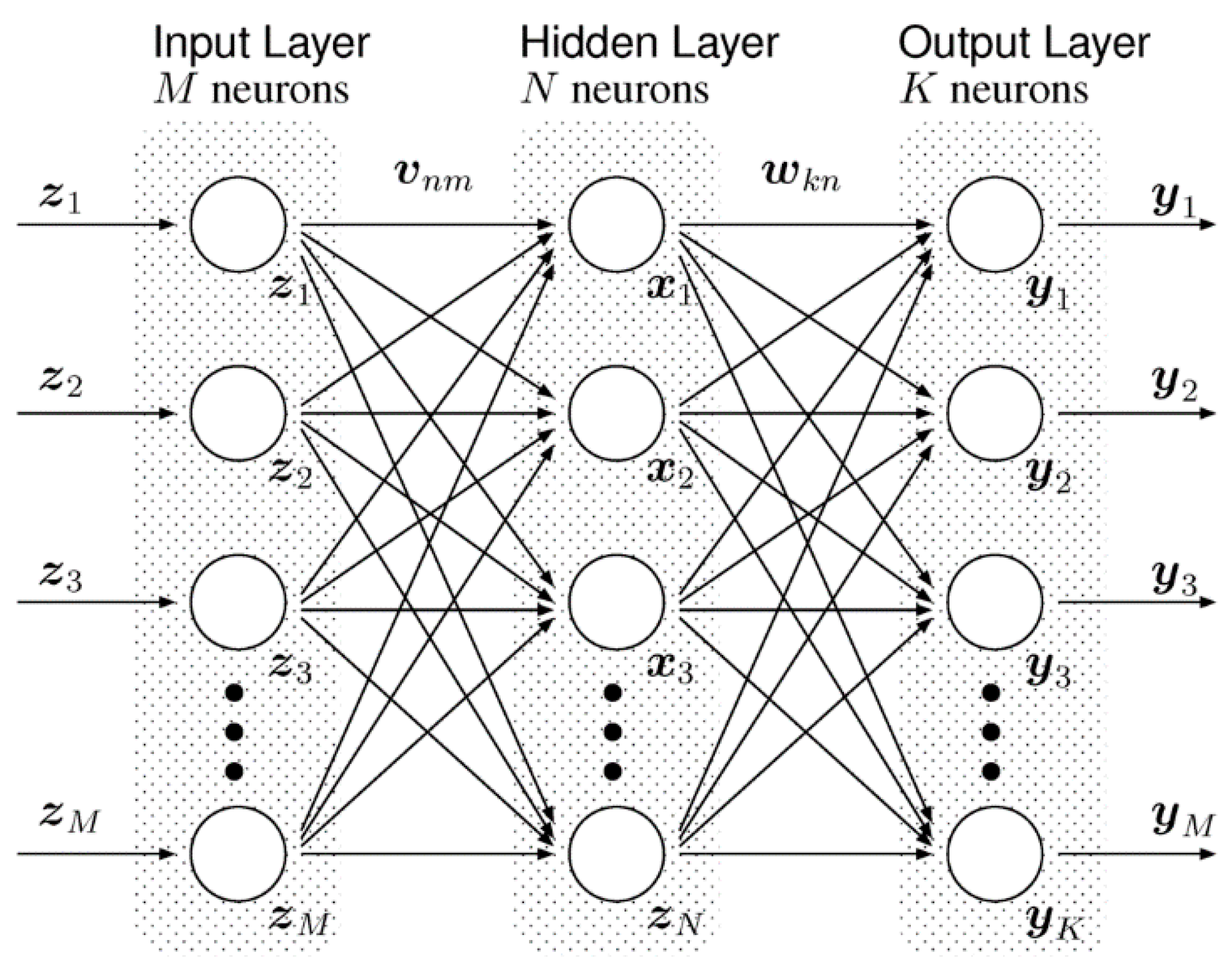
3.1. Artificial Neural Networks
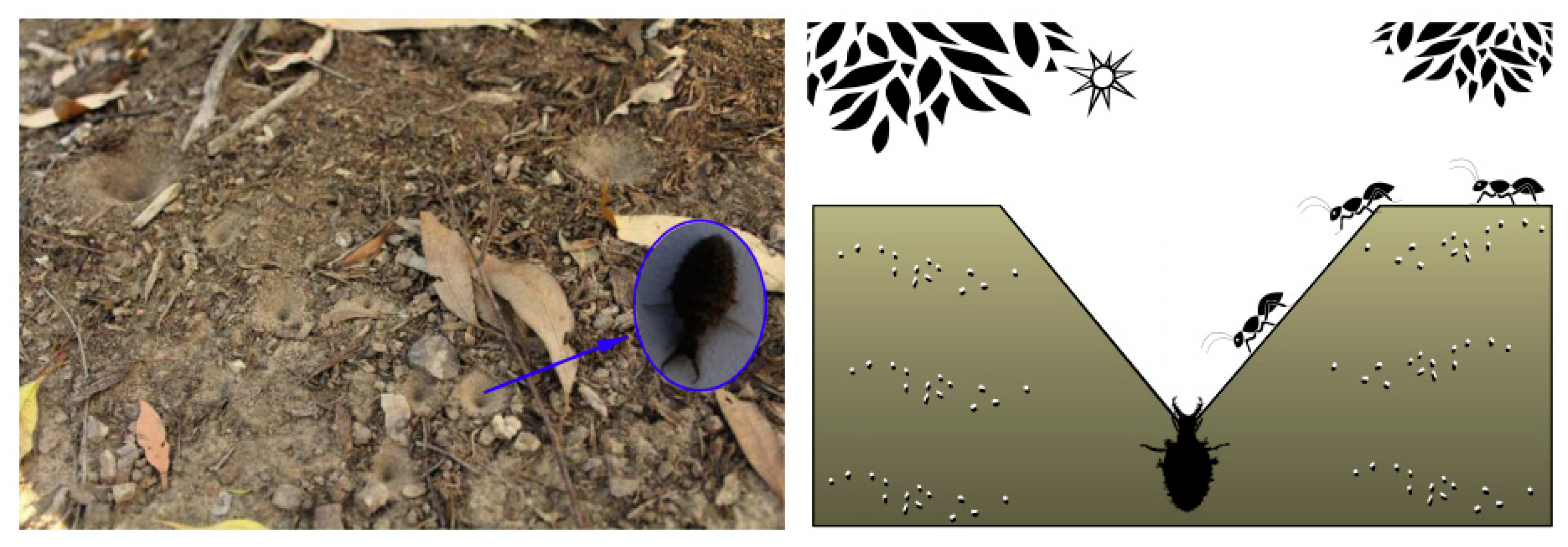
3.2. Ant-Lion Optimizer
- Step 1
- (Initialization Phase): Randomly place M number of ants, and N number of ant-lions over the search space.
- Step 2:
- Calculate the fitness levels of all ants and ant-lions. Additionally, determine the best ant-lion according to the calculated fitness values.
- Step 3:
- Perform the following steps until the stopping criteria is met.
- Step 3.1:
- Perform the following sub-steps for each ant.
- Step 3.1.1:
- Select an ant-lion with the roulette wheel.
- Step 3.1.2:
- Update the minimum and maximum (c and d) values with the ratio (I), by using the following equations:
- Step 3.1.3:
- Perform a random walk (Equation (3)) and normalize it (Equation (4)):where cs is the cumulative sum, and
- Step 3.1.4:
- Update the related ant’s position by using the following equation:where is a random walk around the chosen ant-lion with the roulette wheel while is a random walk around the best ant-lion.
- Step 3.2:
- Calcute the fitness values for all ants.
- Step 3.3:
- Replace an ant-lion with its related ant if it is fitter by using the following equation:
- Step 3.4:
- Update the best ant-lion if an ant-lion is better than it.
- Step 4:
- The best ant-lion is the optimum solution(s) for the related problem.
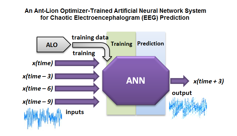
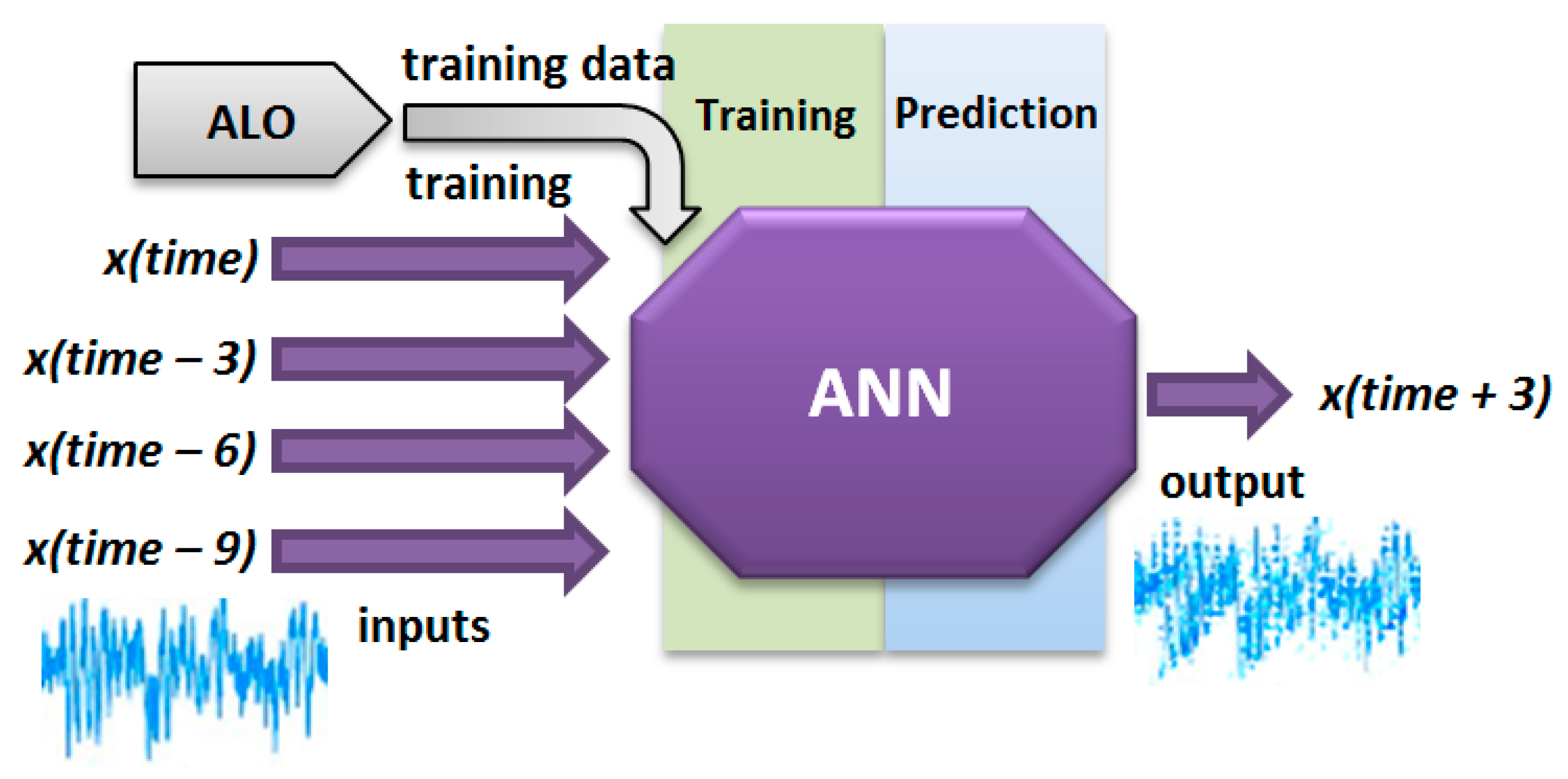
3.3. Chaotic Time Series Prediction with the ANN–ALO System
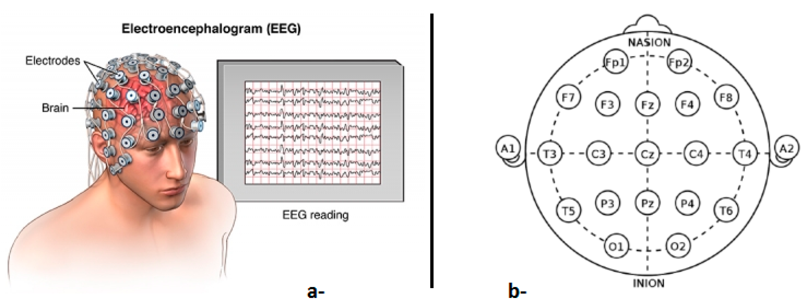
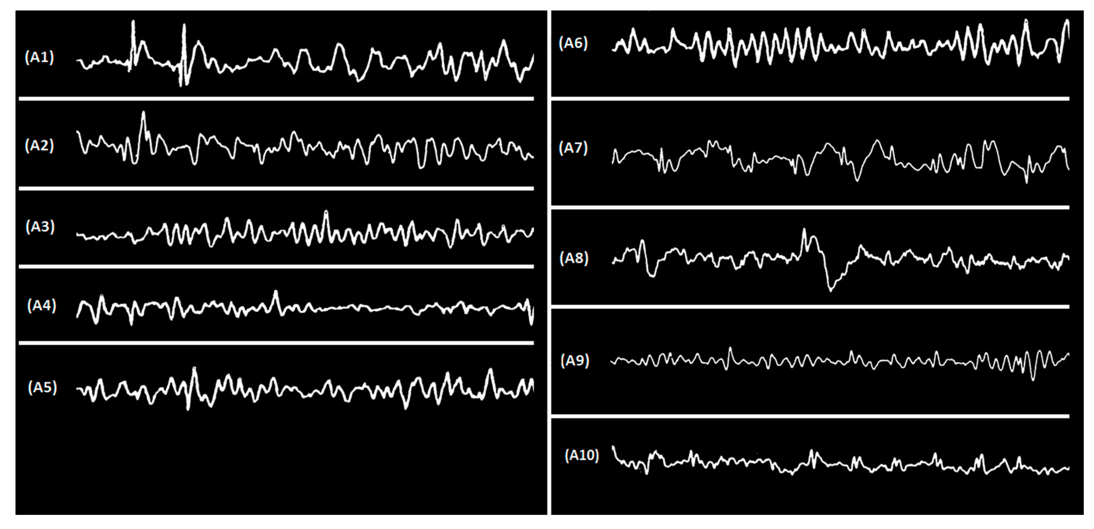
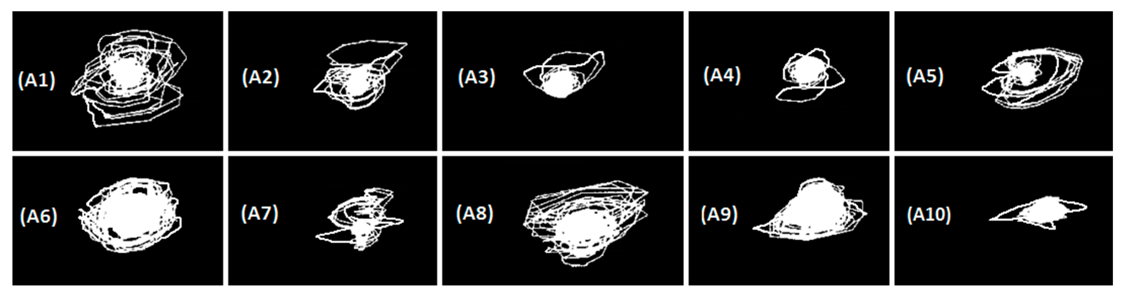
4. Applications on Electroencephalogram (EEG) Prediction
4.1. Chaotic EEG Time Series Prediction with the ANN–ALO System
4.2. Organization of the ANN–ALO
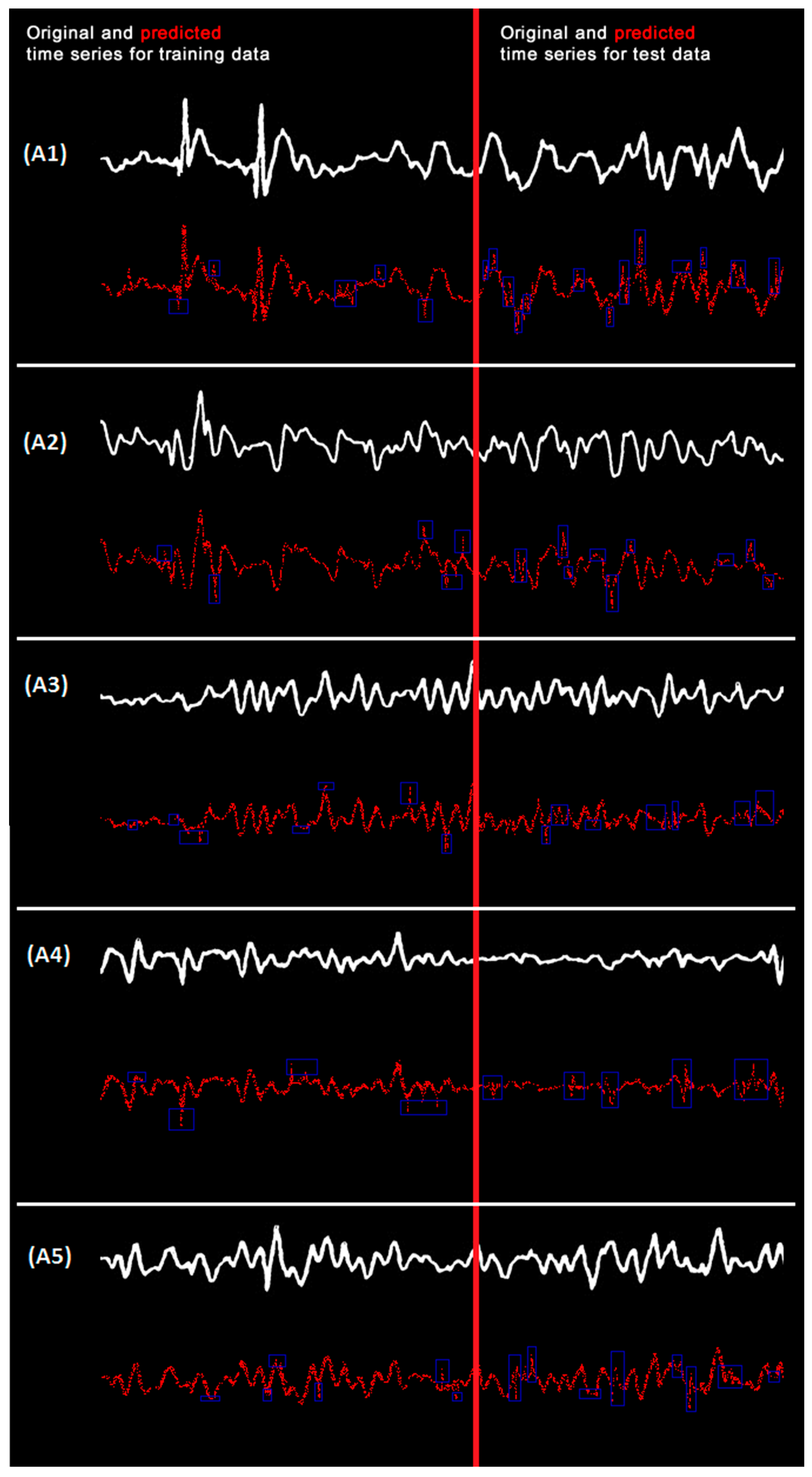
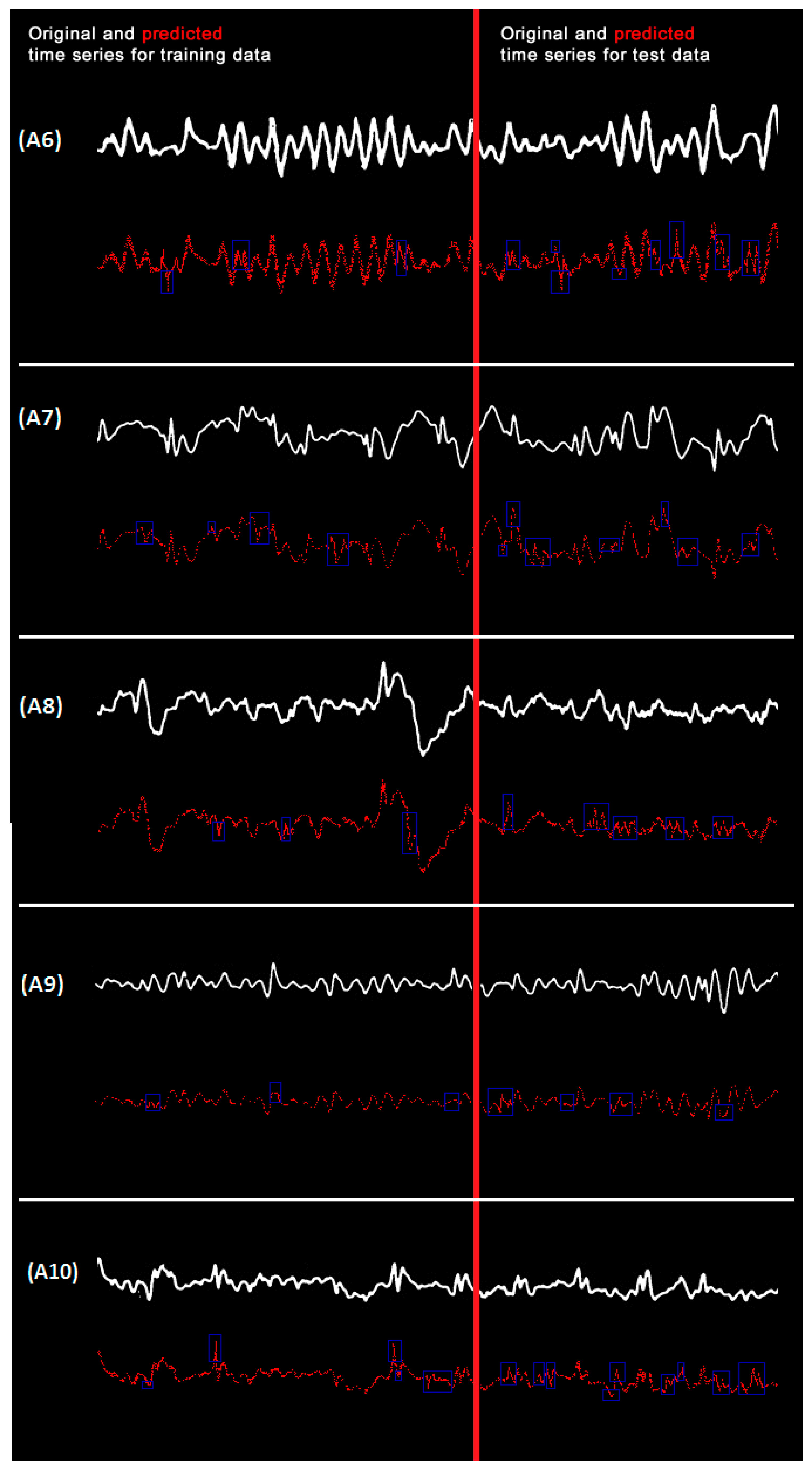
5. Findings from Prediction Applications
6. More Comparisons with Alternative Approaches
6.1. Validation Test
6.2. Ranking
6.3. Practical Application and Experiences by Physicians
7. Discussion
7.1. Discussion over Findings
7.2. General Discussion
8. Conclusions
8.1. Obtained Results
8.2. Future Work
Funding
Conflicts of Interest
References
- Douglas, A.I.; Williams, G.M.; Samuel, A.W.; Carol, A.W. Basic Statistics for Business & Economics, 3rd ed.; McGraw-Hill: New York, NY, USA, 2009. [Google Scholar]
- Esling, P.; Agon, C. Time-series data mining. ACM Comput. Surv. (CSUR) 2012, 45, 12. [Google Scholar] [CrossRef]
- NIST SEMATECH. Introduction to Time Series Analysis. In Engineering Statistics Handbook; NIST: Gaithersburg, MD, USA, 2016. Available online: http://www.itl.nist.gov/div898/handbook/pmc/section4/pmc4.htm (accessed on 10 July 2016).
- Penn State Eberly Collage of Science. Overview of Time Series Characteristics, STAT-510 (App. Time Series Analysis). Available online: https://onlinecourses.science.psu.edu/stat510/node/47 (accessed on 10 July 2016).
- Gromov, G.A.; Shulga, A.N. Chaotic time series prediction with employment of ant colony optimization. Expert Syst. Appl. 2012, 39, 8474–8478. [Google Scholar] [CrossRef]
- Mirjalili, S. The ant lion optimizer. Adv. Eng. Softw. 2015, 83, 80–98. [Google Scholar] [CrossRef]
- Mirjalili, S.; Jangir, P.; Saremi, S. Multi-objective ant lion optimizer: A multi-objective optimization algorithm for solving engineering problems. Appl. Intell. 2017, 46, 79–95. [Google Scholar] [CrossRef]
- Yao, P.; Wang, H. Dynamic Adaptive Ant Lion Optimizer applied to route planning for unmanned aerial vehicle. Soft Comput. 2017, 21, 5475–5488. [Google Scholar] [CrossRef]
- Mani, M.; Bozorg-Haddad, O.; Chu, X. Ant Lion Optimizer (ALO) Algorithm. In Advanced Optimization by Nature-Inspired Algorithms; Springer: Singapore, 2018; pp. 105–116. [Google Scholar]
- Kose, U.; Arslan, A. Forecasting chaotic time series via anfis supported by vortex optimization algorithm: Applications on electroencephalogram time series. Arab. J. Sci. Eng. 2017, 42, 3103–3114. [Google Scholar] [CrossRef]
- Gan, M.; Peng, H.; Peng, X.; Chen, X.; Inoussa, G. A locally linear RBF network-based state-dependent AR model for nonlinear time series modeling. Inf. Sci. 2010, 180, 4370–4383. [Google Scholar] [CrossRef]
- Wong, W.K.; Xia, M.; Chu, W.C. Adaptive neural network model for time-series forecasting. Eur. J. Oper. Res. 2010, 207, 807–816. [Google Scholar] [CrossRef]
- Gentili, P.L.; Gotoda, H.; Dolnik, M.; Epstein, I.R. Analysis and prediction of aperiodic hydrodynamic oscillatory time series by feed-forward neural networks, fuzzy logic, and a local nonlinear predictor. Chaos: An Interdiscip. J. Nonlinear Sci. 2015, 25, 013104. [Google Scholar] [CrossRef] [PubMed]
- Chen, D.; Han, W. Prediction of multivariate chaotic time series via radial basis function neural network. Complexity 2013, 18, 55–66. [Google Scholar] [CrossRef]
- Wu, X.; Li, C.; Wang, Y.; Zhu, Z.; Liu, W. Nonlinear time series prediction using iterated extended Kalman filter trained single multiplicative neuron model. J. Inf. Comput. Sci. 2013, 10, 385–393. [Google Scholar]
- Yadav, R.N.; Kalra, P.K.; John, J. Time series prediction with single multiplicative neuron model. Appl. Soft Comput. 2007, 7, 1157–1163. [Google Scholar] [CrossRef]
- Zhao, L.; Yang, Y. PSO-based single multiplicative neuron model for time series prediction. Expert Syst. Appl. 2009, 36, 2805–2812. [Google Scholar] [CrossRef]
- Yao, J.; Liu, W. Nonlinear time series prediction of atmospheric visibility in shanghai. In Time Series Analysis, Modeling and Applications; Intelligent Systems Reference Library; Pedrycz, W., Chen, S.-M., Eds.; Springer: Berlin/Heidelberg, Germany, 2013; Volume 47. [Google Scholar]
- Unler, A. Improvement of energy demand forecasts using swarm intelligence: The case of Turkey with projections to 2025. Energy Policy 2008, 36, 1937–1944. [Google Scholar] [CrossRef]
- Porto, A.; Irigoyen, E.; Larrea, M. A PSO boosted ensemble of extreme learning machines for time series forecasting. In The 13th International Conference on Soft Computing Models in Industrial and Environmental Applications; Springer International Publishing AG: Cham, Switzerland, 2018; pp. 324–333. [Google Scholar]
- Weng, S.S.; Liu, Y.H. Mining time series data for segmentation by using ant colony optimization. Eur. J. Oper. Res. 2006, 173, 921–937. [Google Scholar] [CrossRef]
- Toskari, M.D. Estimating the net electricity energy generation and demand using the ant colony optimization approach. Energy Policy 2009, 37, 1181–1187. [Google Scholar]
- Hong, W.C. Application of chaotic ant swarm optimization in electric load forecasting. Energy Policy 2010, 38, 5830–5839. [Google Scholar] [CrossRef]
- Niu, D.; Wang, Y.; Wu, D.D. Power load forecasting using support vector machine and ant colony optimization. Expert Syst. Appl. 2010, 37, 2531–2539. [Google Scholar] [CrossRef]
- Yeh, W.-C. New parameter-free simplified swarm optimization for artificial neural network training and its application in the prediction of time series. IEEE Trans. Neural Netw. Learn. Syst. 2013, 24, 661–665. [Google Scholar] [PubMed]
- Nourani, V.; Andalib, G. Wavelet based Artificial Intelligence approaches for prediction of hydrological time series. In Proceedings of the Australasian Conference on Artificial Life and Computational Intelligence, Newcastle, NSW, Australia, 5–7 February 2015; pp. 422–435. [Google Scholar]
- Bontempi, G.; Taieb, S.B.; Le Borgne, Y.-A. Machine learning strategies for time series forecasting. In Business Intelligence; Lecture Notes in Business Information Processing; Aufaure, M.-A., Zimanyi, E., Eds.; Springer: Berlin/Heidelberg, Germany, 2013; Volume 138. [Google Scholar]
- Hu, Y.X.; Zhang, H.T. Prediction of the chaotic time series based on chaotic simulated annealing and support vector machine. In Proceedings of the International Conference on Solid State Devices and Materials Science, Macao, China, 1–2 April 2012; pp. 506–512. [Google Scholar]
- Liu, P.; Yao, J.A. Application of least square support vector machine based on particle swarm optimization to chaotic time series prediction. In Proceedings of the IEEE International Conference on Intelligent Computing and Intelligent Systems, Shanghai, China, 20–22 November 2009; pp. 458–462. [Google Scholar]
- Quian, J.S.; Cheng, J.; Guo, Y.N. A novel multiple support vector machines architecture for chaotic time series prediction. In Proceedings of the ICNC: International Conference on Natural Computation, Xi’an, China, 24–28 September 2006; Volume 4221, pp. 147–156. [Google Scholar]
- Yang, Z.H.O.; Wang, Y.S.; Li, D.D.; Wang, C.J. Predict the time series of the parameter-varying chaotic system based on reduced recursive lease square support vector machine. In Proceedings of the IEEE International Conference on Artificial Intelligence and Computational Intelligence, Shanghai, China, 7–8 November 2009; pp. 29–34. [Google Scholar]
- Zhang, J.S.; Dang, J.L.; Li, H.C. Local support vector machine prediction of spatiotemporal chaotic time series. Acta Phys. Sin. 2007, 56, 67–77. [Google Scholar]
- Farooq, T.; Guergachi, A.; Krishnan, S. Chaotic time series prediction using knowledge based Green’s kernel and least-squares support vector machines. In Proceedings of the IEEE International Conference on Systems, Man and Cybernetics, Montreal, QC, Canada, 7–10 October 2007; pp. 2669–2674. [Google Scholar]
- Shi, Z.W.; Han, M. Support vector echo-state machine for chaotic time-series prediction. IEEE Trans. Neural Netw. 2007, 18, 359–372. [Google Scholar] [CrossRef] [PubMed]
- Li, H.T.; Zhang, X.F. Precipitation time series predicting of the chaotic characters using support vector machines. In Proceedings of the International Conference on Information Management, Innovation Management and Industrial Engineering, Xi’an, China, 26–27 December 2009; pp. 407–410. [Google Scholar]
- Zhu, C.H.; Li, L.L.; Li, J.H.; Gao, J.S. Short-term wind speed forecasting by using chaotic theory and SVM. Appl. Mech. Mater. 2013, 300–301, 842–847. [Google Scholar] [CrossRef]
- Ren, C.-X.; Wang, C.-B.; Yin, C.-C.; Chen, M.; Shan, X. The prediction of short-term traffic flow based on the niche genetic algorithm and BP neural network. In Proceedings of the 2012 International Conference on Information Technology and Software Engineering, Beijing, China, 8–10 December 2012; pp. 775–781. [Google Scholar]
- Ding, C.; Wang, W.; Wang, X.; Baumann, M. A neural network model for driver’s lane-changing trajectory prediction in urban traffic flow. Math. Probl. Eng. 2013. [Google Scholar] [CrossRef]
- Yin, H.; Wong, S.C.; Xu, J.; Wong, C.K. Urban traffic flow prediction using a fuzzy-neural approach. Transp. Res. Part C Emerg. Technol. 2002, 10, 85–98. [Google Scholar] [CrossRef]
- Dunne, S.; Ghosh, B. Weather adaptive traffic prediction using neurowavelet models. IEEE Trans. Intell. Transp. Syst. 2013, 14, 370–379. [Google Scholar] [CrossRef]
- Pulido, M.; Melin, P.; Castillo, O. Particle swarm optimization of ensemble neural networks with fuzzy aggregation for time series prediction of the Mexican Stock Exchange. Inf. Sci. 2014, 280, 188–204. [Google Scholar] [CrossRef]
- Huang, D.Z.; Gong, R.X.; Gong, S. Prediction of wind power by chaos and BP artificial neural networks approach based on genetic algorithm. J. Electr. Eng. Technol. 2015, 10, 41–46. [Google Scholar] [CrossRef]
- Jiang, P.; Qin, S.; Wu, J.; Sun, B. Time series analysis and forecasting for wind speeds using support vector regression coupled with artificial intelligent algorithms. Math. Probl. Eng. 2015, 2015, 939305. [Google Scholar] [CrossRef]
- Doucoure, B.; Agbossou, K.; Cardenas, A. Time series prediction using artificial wavelet neural network and multi-resolution analysis: Application to wind speed data. Renew. Energy 2016, 92, 202–211. [Google Scholar] [CrossRef]
- Chandra, R. Competition and collaboration in cooperative coevolution of Elman recurrent neural networks for time-series prediction. IEEE Trans. Neural Netw. Learn. Syst. 2015, 26, 3123–3136. [Google Scholar] [CrossRef] [PubMed]
- Chai, S.H.; Lim, J.S. Forecasting business cycle with chaotic time series based on neural network with weighted fuzzy membership functions. Chaos Solitons Fractals 2016, 90, 118–126. [Google Scholar] [CrossRef]
- Seo, Y.; Kim, S.; Kisi, O.; Singh, V.P. Daily water level forecasting using wavelet decomposition and Artificial Intelligence techniques. J. Hydrol. 2015, 520, 224–243. [Google Scholar] [CrossRef]
- Marzban, F.; Ayanzadeh, R.; Marzban, P. Discrete time dynamic neural networks for predicting chaotic time series. J. Artif. Intell. 2014, 7, 24. [Google Scholar] [CrossRef]
- Okkan, U. Wavelet neural network model for reservoir inflow prediction. Sci. Iran. 2012, 19, 1445–1455. [Google Scholar] [CrossRef]
- Zhou, T.; Gao, S.; Wang, J.; Chu, C.; Todo, Y.; Tang, Z. Financial time series prediction using a dendritic neuron model. Knowl.-Based Syst. 2016, 105, 214–224. [Google Scholar] [CrossRef]
- Wang, L.; Zou, F.; Hei, X.; Yang, D.; Chen, D.; Jiang, Q.; Cao, Z. A hybridization of teaching–learning-based optimization and differential evolution for chaotic time series prediction. Neural Comput. Appl. 2014, 25, 1407–1422. [Google Scholar] [CrossRef]
- Heydari, G.; Vali, M.; Gharaveisi, A.A. Chaotic time series prediction via artificial neural square fuzzy inference system. Expert Syst. Appl. 2016, 55, 461–468. [Google Scholar] [CrossRef]
- Wang, L.; Zeng, Y.; Chen, T. Back propagation neural network with adaptive differential evolution algorithm for time series forecasting. Expert Syst. Appl. 2015, 42, 855–863. [Google Scholar] [CrossRef]
- Catalao, J.P.S.; Pousinho, H.M.I.; Mendes, V.M.F. Hybrid wavelet-PSO-ANFIS approach for short-term electricity prices forecasting. IEEE Trans. Power Syst. 2011, 26, 137–144. [Google Scholar] [CrossRef]
- Patra, A.; Das, S.; Mishra, S.N.; Senapati, M.R. An adaptive local linear optimized radial basis functional neural network model for financial time series prediction. Neural Comput. Appl. 2017, 28, 101–110. [Google Scholar] [CrossRef]
- Ravi, V.; Pradeepkumar, D.; Deb, K. Financial time series prediction using hybrids of chaos theory, multi-layer perceptron and multi-objective evolutionary algorithms. Swarm Evol. Comput. 2017, 36, 136–149. [Google Scholar] [CrossRef]
- Méndez, E.; Lugo, O.; Melin, P. A competitive modular neural network for long-term time series forecasting. In Nature-Inspired Design of Hybrid Intelligent Systems; Springer International Publishing: Cham, Switzerland, 2017; pp. 243–254. [Google Scholar]
- Wei, B.L.; Luo, X.S.; Wang, B.H.; Guo, W.; Fu, J.J. Prediction of EEG signal by using radial basis function neural networks. Chin. J. Biomed. Eng. 2003, 22, 488–492. [Google Scholar]
- Hou, M.-Z.; Han, X.-L.; Huang, X. Application of BP neural network for forecast of EEG signal. Comput. Eng. Des. 2006, 14, 061. [Google Scholar]
- Wei, C.; Zhang, C.; Wu, M. A study on the universal method of EEG and ECG prediction. In Proceedings of the 2017 10th International Congress on Image and Signal Processing, BioMedical Engineering and Informatics (CISP-BMEI), Shanghai, China, 14–16 October 2017; IEEE: Piscataway, NJ, USA, 2017; pp. 1–5. [Google Scholar]
- Blinowska, K.J.; Malinowski, M. Non-linear and linear forecasting of the EEG time series. Biol. Cybern. 1991, 66, 159–165. [Google Scholar] [CrossRef] [PubMed]
- Lin, W.B.; Shu, L.X.; Hong, W.B.; Jun, Q.H.; Wei, G.; Jie, F.J. A method based on the third-order Volterra filter for adaptive predictions of chaotic time series. Acta Phys. Sin. 2002, 10, 006. [Google Scholar]
- Coyle, D.; Prasad, G.; McGinnity, T.M. A time-series prediction approach for feature extraction in a brain-computer interface. IEEE Trans. Neural Syst. Rehabil. Eng. 2005, 13, 461–467. [Google Scholar] [CrossRef] [PubMed]
- Coelho, V.N.; Coelho, I.M.; Coelho, B.N.; Souza, M.J.; Guimarães, F.G.; Luz, E.D.S.; Barbosa, A.C.; Coelho, M.N.; Netto, G.G.; Costa, R.C.; et al. EEG time series learning and classification using a hybrid forecasting model calibrated with GVNS. Electron. Notes Discret. Math. 2017, 58, 79–86. [Google Scholar] [CrossRef]
- Komijani, H.; Nabaei, A.; Zarrabi, H. Classification of normal and epileptic EEG signals using adaptive neuro-fuzzy network based on time series prediction. Neurosci. Biomed. Eng. 2016, 4, 273–277. [Google Scholar] [CrossRef]
- Prasad, S.C.; Prasad, P. Deep recurrent neural networks for time series prediction. arXiv, 2014; arXiv:1407.5949. [Google Scholar]
- Forney, E.M. Electroencephalogram Classification by Forecasting with Recurrent Neural Networks. Master’s Dissertation, Department of Computer Science, Colorado State University, Fort Collins, CO, USA, 2011. [Google Scholar]
- Carpenter, G.A. Neural network models for pattern recognition and associative memory. Neural Netw. 1989, 2, 243–257. [Google Scholar] [CrossRef]
- Cochocki, A.; Unbehauen, R. Neural Networks for Optimization and Signal Processing; John Wiley & Sons, Inc.: Chichester, UK, 1993. [Google Scholar]
- Miller, W.T.; Sutton, R.S.; Werbos, P.J. Neural Networks for Control; MIT Press: Cambridge, MA, USA, 1995. [Google Scholar]
- Ripley, B.D. Neural networks and related methods for classification. J. R. Stat. Soc. Ser. B 1994, 56, 409–456. [Google Scholar]
- Basheer, I.A.; Hajmeer, M. Artificial neural networks: Fundamentals, computing, design and application. J. Microbiol. Methods 2000, 43, 3–31. [Google Scholar] [CrossRef]
- Badri, A.; Ameli, Z.; Birjandi, A.M. Application of artificial neural networks and fuzzy logic methods for short term load forecasting. Energy Procedia 2012, 14, 1883–1888. [Google Scholar] [CrossRef]
- Ghorbanian, J.; Ahmadi, M.; Soltani, R. Design predictive tool and optimization of journal bearing using neural network model and multi-objective genetic algorithm. Sci. Iran. 2011, 18, 1095–1105. [Google Scholar] [CrossRef]
- Gholizadeh, S.; Seyedpoor, S.M. Shape optimization of arch dams by metaheuristics and neural networks for frequency constraints. Sci. Iran. 2011, 18, 1020–1027. [Google Scholar] [CrossRef]
- Firouzi, A.; Rahai, A. An integrated ANN-GA for reliability based inspection of concrete bridge decks considering extent of corrosion-induced cracks and life cycle costs. Sci. Iran. 2012, 19, 974–981. [Google Scholar] [CrossRef]
- Shahreza, M.L.; Moazzami, D.; Moshiri, B.; Delavar, M.R. Anomaly detection using a self-organizing map and particle swarm optimization. Sci. Iran. 2011, 18, 1460–1468. [Google Scholar] [CrossRef]
- Isokawa, T.; Nishimura, H.; Matsui, N. Quaternionic multilayer perceptron with local analyticity. Information 2012, 3, 756–770. [Google Scholar] [CrossRef]
- Kose, U.; Arslan, A. Optimization of self-learning in Computer Engineering courses: An intelligent software system supported by Artificial Neural Network and Vortex Optimization Algorithm. Comput. Appl. Eng. Educ. 2017, 25, 142–156. [Google Scholar] [CrossRef]
- McCulloch, W.S.; Pitts, W. A logical calculus of the ideas immanent in nervous activity. Bull. Math. Biophys. 1990, 5, 115–133. [Google Scholar] [CrossRef]
- Anderson, D.; McNeill, G. Artificial Neural Networks Technology; A DACS State-of-the-Art Report; Kaman Sciences Corporation: Utica, NY, USA, 1992. [Google Scholar]
- Ugur, A.; Kinaci, A.C. A web-based tool for teaching neural network concepts. Comput. Appl. Eng. Educ. 2010, 18, 449–457. [Google Scholar] [CrossRef]
- Yegnanarayana, B. Artificial Neural Networks; PHI Learning Pvt. Ltd.: Delhi, India, 2009. [Google Scholar]
- Raju, M.; Saikia, L.C.; Sinha, N. Automatic generation control of a multi-area system using ant lion optimizer algorithm based PID plus second order derivative controller. Int. J. Electr. Power Energy Syst. 2016, 80, 52–63. [Google Scholar] [CrossRef]
- Kamboj, V.K.; Bhadoria, A.; Bath, S.K. Solution of non-convex economic load dispatch problem for small-scale power systems using ant lion optimizer. Neural Comput. Appl. 2017, 28, 2181–2192. [Google Scholar] [CrossRef]
- Yamany, W.; Tharwat, A.; Hassanin, M.F.; Gaber, T.; Hassanien, A.E.; Kim, T.H. A new multi-layer perceptrons trainer based on ant lion optimization algorithm. In Proceedings of the 2015 Fourth International Conference on Information Science and Industrial Applications (ISI), Busan, Korea, 20–22 September 2015; IEEE: Piscataway, NJ, USA, 2015; pp. 40–45. [Google Scholar]
- Maher, M.; Ebrahim, M.A.; Mohamed, E.A.; Mohamed, A. Ant-lion Optimizer Based Optimal Allocation of Distributed Generators in Radial Distribution Networks. Int. J. Eng. Inf. Syst. 2017, 1, 225–238. [Google Scholar]
- Kilic, H.; Yuzgec, U. Improved antlion optimization algorithm via tournament selection. In Proceedings of the 2017 9th International Conference on Computational Intelligence and Communication Networks (CICN), Girne, Cyprus, 16–17 September 2017; IEEE: Piscataway, NJ, USA, 2017; pp. 200–205. [Google Scholar]
- Ali, A.H.; Youssef, A.R.; George, T.; Kamel, S. Optimal DG allocation in distribution systems using Ant lion optimizer. In Proceedings of the 2018 International Conference on Innovative Trends in Computer Engineering (ITCE), Aswan, Egypt, 19–21 February 2018; IEEE: Piscataway, NJ, USA, 2018; pp. 324–331. [Google Scholar]
- Pradhan, R.; Majhi, S.K.; Pradhan, J.K.; Pati, B.B. Performance Evaluation of PID Controller for an Automobile Cruise Control System using Ant Lion Optimizer. Eng. J. 2017, 21, 347–361. [Google Scholar] [CrossRef]
- Rajan, A.; Jeevan, K.; Malakar, T. Weighted elitism based Ant Lion Optimizer to solve optimum VAr planning problem. Appl. Soft Comput. 2017, 55, 352–370. [Google Scholar] [CrossRef]
- Blum, C.; Li, X. Swarm intelligence in optimization. In Swarm Intelligence; Blum, C., Merkle, D., Eds.; Springer: Berlin/Heidelberg, Germany, 2008. [Google Scholar]
- Engelbrecht, A.P. Fundamentals of Computational Swarm Intelligence; John Wiley & Sons: Hoboken, NJ, USA, 2006. [Google Scholar]
- Bonabeau, E.; Dorigo, M.; Theraulaz, G. Swarm Intelligence: From Natural to Artificial Systems (No. 1); Oxford University Press: Oxford, UK, 1999. [Google Scholar]
- Panigrahi, B.K.; Shi, Y.; Lim, M.H. (Eds.) Handbook of Swarm Intelligence: Concepts, Principles and Applications; Springer Science & Business Media: Berlin, Germany, 2011; Volume 8. [Google Scholar]
- Fukuyama, Y. Fundamentals of particle swarm optimization techniques. In Modern Heuristic Optimization Techniques: Theory and Applications to Power Systems; Lee, K.Y., El-Sharkawi, M.A., Eds.; John Wiley & Sons: Hoboken, NJ, USA, 2008. [Google Scholar]
- Bonabeau, E.; Dorigo, M.; Theraulaz, G. Inspiration for optimization from social insect behaviour. Nature 2000, 406, 39–42. [Google Scholar] [CrossRef] [PubMed]
- Kennedy, J. Particle swarm optimization. In Encyclopedia of Machine Learning; Sammut, C., Webb, G.I., Eds.; Springer: New York, NY, USA, 2011. [Google Scholar]
- Dorigo, M.; Blum, C. Ant colony optimization theory: A survey. Theor. Comput. Sci. 2005, 344, 243–278. [Google Scholar] [CrossRef]
- Karaboga, D. Artificial Intelligence Optimization Algorithms; Nobel Publishing: Ankara, Turkey, 2004; ISBN 975-6574. (In Turkish) [Google Scholar]
- Kose, U. Development of Artificial Intelligence Based Optimization Algorithms. Ph.D. Thesis, nstitute of Natural Sciences, Department of Computer Engineering, Selcuk University, Konya, Turkey, 2017. (In Turkish). [Google Scholar]
- MyScienceSchool.org. What Is Electroencephalography (EEG)? Available online: http://myscienceschool.org/index.php?/archives/3208-What-is-Electroencephalography-EEG.html (accessed on 10 March 2017).
- Sjölie, D. Reality-Based Brain-Computer Interaction. Ph.D. Thesis, Department of Computing Science, Umeå University, Umeå, Sweden, 2011. Available online: https://www.researchgate.net/publication/215509007_Reality-Based_Brain-Computer_Interaction (accessed on 10 March 2017).
- Jadhav, P.; Shanamugan, D.; Chourasia, A.; Ghole, A.R.; Acharyya, A.; Naik, G.R. Automated detection and correction of eye blink and muscular artefacts in EEG signal for analysis of Autism Spectrum Disorder. In Proceedings of the 2014 36th Annual International Conference of the IEEE Engineering in Medicine and Biology Society (EMBC 2014), Chicago, IL, USA, 26–30 August 2014; pp. 1881–1884. [Google Scholar]
- Sandri, M. Numerical calculation of Lyapunov exponents. Math. J. 1996, 6, 78–84. [Google Scholar]
- Bishop, C.M. Neural Networks for Pattern Recognition; Oxford University Press: Oxford, UK, 1995. [Google Scholar]
- OTexts.org. Evaluating Forecast Accuracy. Available online: https://www.otexts.org/fpp/2/5 (accessed on 16 July 2016).
- Willmott, C.J.; Matsuura, K. Advantages of the mean absolute error (MAE) over the root mean square error (RMSE) in assessing average model performance. Clim. Res. 2005, 30, 79–82. [Google Scholar] [CrossRef]
- Eberhart, R.C.; Kennedy, J. A new optimizer using particle swarm theory. In Proceedings of the Sixth International Symposium on Micro Machine and Human Science, Nagoya, Japan, 4–6 October 1995; pp. 39–43. [Google Scholar]
- Kennedy, J. The particle swarm: Social adaptation of knowledge. In Proceedings of the 1997 IEEE International Conference on Evolutionary Computation, Indianapolis, IN, USA, 13–16 April 1997; IEEE: Piscataway, NJ, USA, 1997; pp. 303–308. [Google Scholar]
- Yang, X.S.; Deb, S. Cuckoo search via Lévy flights. In Proceedings of the 2009 World Congress on Nature & Biologically Inspired Computing, Coimbatore, India, 9–11 December 2009; IEEE: Piscataway, NJ, USA, 2009; pp. 210–214. [Google Scholar]
- Yang, X.S.; Deb, S. Cuckoo search: Recent advances and applications. Neural Comput. Appl. 2014, 24, 169–174. [Google Scholar] [CrossRef]
- Yang, X.S. Nature-Inspired Metaheuristic Algorithms; Luniver Press: Frome, UK, 2010. [Google Scholar]
- Yang, X.S. Firefly algorithms for multimodal optimization. In Stochastic Algorithms: Foundations and Applications; Watanabe, O., Zeugmann, T., Eds.; Springer: Berlin/Heidelberg, Germany, 2009. [Google Scholar]
- Yang, X.S. A new metaheuristic bat-inspired algorithm. In Nature Inspired Cooperative Strategies for Optimization (NICSO 2010); González, J.R., Pelta, D.A., Cruz, C., Terrazas, G., Krasnogor, N., Eds.; Springer: Berlin/Heidelberg, Germany, 2010. [Google Scholar]
- Yang, X.S.; Hossein Gandomi, A. Bat algorithm: A novel approach for global engineering optimization. Eng. Comput. 2012, 29, 464–483. [Google Scholar] [CrossRef]
- Chauvin, Y.; Rumelhart, D.E. Backpropagation: Theory, Architectures, and Applications; Psychology Press: Hillsdale, NJ, USA, 2013. [Google Scholar]
- Dasgupta, S.; Osogami, T. Nonlinear Dynamic Boltzmann Machines for Time-Series Prediction. In Proceedings of the AAAI, San Francisco, CA, USA, 4–9 February 2017; pp. 1833–1839. [Google Scholar]
- Kim, K.J. Financial time series forecasting using support vector machines. Neurocomputing 2003, 55, 307–319. [Google Scholar] [CrossRef]
- Hassan, M.R.; Nath, B. Stock market forecasting using hidden Markov model: A new approach. In Proceedings of the 5th International Conference on Intelligent Systems Design and Applications 2005. ISDA ’05, Warsaw, Poland, 8–10 September 2005; IEEE: Piscataway, NJ, USA, 2005; pp. 192–196. [Google Scholar]
- Brahim-Belhouari, S.; Bermak, A. Gaussian process for nonstationary time series prediction. Comput. Stat. Data Anal. 2004, 47, 705–712. [Google Scholar] [CrossRef]
- Ediger, V.Ş.; Akar, S. ARIMA forecasting of primary energy demand by fuel in Turkey. Energy Policy 2007, 35, 1701–1708. [Google Scholar] [CrossRef]
- Poggi, P.; Muselli, M.; Notton, G.; Cristofari, C.; Louche, A. Forecasting and simulating wind speed in Corsica by using an autoregressive model. Energy Convers. Manag. 2003, 44, 3177–3196. [Google Scholar] [CrossRef]
- Larose, D.T.; Larose, C.D. K-nearest neighbor algorithm. In Discovering Knowledge in Data: An Introduction to Data Mining, 2nd ed.; Wiley: Hoboken, NJ, USA, 2005; pp. 149–164. [Google Scholar]
- Giacomini, R.; White, H. Tests of conditional predictive ability. Econometrica 2006, 74, 1545–1578. [Google Scholar] [CrossRef]
- Giarratano, J.C.; Riley, G. Expert Systems; PWS Publishing, Co.: Boston, MA, USA, 1998. [Google Scholar]
- Turban, E.; Frenzel, L.E. Expert Systems and Applied Artificial Intelligence; Prentice Hall Professional Technical Reference; ACM Digital Library: New York, NY, USA, 1992. [Google Scholar]
- David, J.M.; Krivine, J.P.; Simmons, R. (Eds.) Second Generation Expert Systems; Springer Science & Business Media: Berlin, Germany; New York, NY, USA, 2012. [Google Scholar]
- Guerlain, S.; Smith, P.J.; Smith, J.W.; Rudmann, S.; Obradovich, J.; Strohm, P. Decision Support in Medical Systems. In Automation and Human Performance: Theory and Applications; CRC Press: Boca Raton, FL, USA, 1996; pp. 385–406. [Google Scholar]
- Musen, M.A.; Middleton, B.; Greenes, R.A. Clinical decision-support systems. In Biomedical Informatics; Springer: London, UK, 2014; pp. 643–674. [Google Scholar]


| Application (EEG Time Series) | Lyapunov Exponent 1 | Lyapunov Exponent 2 | Lyapunov Exponent 3 |
|---|---|---|---|
| A1 | 0.6515 × 10⁻³ | 0.5078 × 10⁻⁴ | −0.7469 × 10⁻³ |
| A2 | 0.2002 × 10⁻³ | −0.2354 × 10⁻⁴ | −0.4054 × 10⁻³ |
| A3 | −0.0480 × 10⁻³ | −0.9309 × 10⁻⁴ | 0.8753 × 10⁻³ |
| A4 | 0.2552 × 10⁻³ | −0.2734 × 10⁻⁴ | 0.5395 × 10⁻³ |
| A5 | 0.4205 × 10⁻³ | 0.5442 × 10⁻⁴ | −0.0385 × 10⁻³ |
| A6 | −0.8610 × 10⁻³ | 0.7984 × 10⁻⁴ | −0.1260 × 10⁻³ |
| A7 | 0.1245 × 10⁻³ | −0.0166 × 10⁻⁴ | 0.2455 × 10⁻³ |
| A8 | −0.3045 × 10⁻³ | 0.7614 × 10⁻⁴ | 0.3279 × 10⁻³ |
| A9 | 0.6972 × 10⁻³ | −0.1718 × 10⁻⁴ | 0.9491 × 10⁻³ |
| A10 | 0.2330 × 10⁻³ | −0.4401 × 10⁻⁴ | −0.8605 × 10⁻³ |
| ANN–BPA Model No. | Values of ANN Input Neurons | Value of ANN Output Neuron | Total Hidden Layers | Total Neurons in Each Hidden Layer | Average True Prediction Rate |
|---|---|---|---|---|---|
| 1 | x(time); x(time − 3); x(time − 6) [10] | x(time + 3) | 3 | 5 | 88.58% |
| 2 | x(time − 2); x(time − 2); x(time − 3); x(time − 4); [65] | x(time + 2) | 3 | 6 | 90.63% |
| 3 | x(time); x(time − 3); x(time − 6); x(time − 9) | x(time + 3) | 3 | 7 | 93.81% |
| 4 | x(time); x(time − 2); x(time − 4) | x(time + 2) | 4 | 7 | 79.84% |
| 5 | x(time); x(time − 3); x(time − 6); x(time − 9) | x(time + 3) | 4 | 6 | 84.19% |
| Total Neurons in the Input Layer | Values of ANN Input Neurons | Total Neurons in the Output Layer | Value of ANN Output Neuron | Total Hidden Layers | Total Neurons in Each Hidden Layer | Activation Function |
|---|---|---|---|---|---|---|
| 4 | x(time); x(time −3); x(time − 6); x(time − 9) | 1 | x(time + 3) | 3 | 7 | Sigmoid |
| Parameters | Adjust. 1 (ALO-A1) | Adjust. 2 (ALO-A2) | Adjust. 3 (ALO-A3) | Adjust. 4 (ALO-A4) | Adjust. 5 (ALO-A5) |
|---|---|---|---|---|---|
| Number of ant-lions (particles) | 50 | 75 | 100 | 100 | 125 |
| Total iterations (stopping criteria) | 2000 | 3000 | 4000 | 5000 | 6000 |
| Application (EEG Time Series) | ANN–ALO System Including ALO with Different Adjustment | ||||
|---|---|---|---|---|---|
| ALO-A1 | ALO-A2 | ALO-A3 | ALO-A4 | ALO-A5 | |
| A1 | 12.4531 | 12.2219 | 11.2195 | 11.0653 | 12.1029 |
| A2 | 13.8490 | 14.5119 | 13.3933 | 12.9048 | 12.6544 |
| A3 | 15.8722 | 16.6799 | 15.4337 | 14.1190 | 15.3290 |
| A4 | 12.6193 | 11.0907 | 10.8994 | 10.7726 | 11.1167 |
| A5 | 16.3980 | 17.8881 | 16.2110 | 14.3851 | 15.2962 |
| A6 | 13.1566 | 14.8791 | 12.1109 | 12.9671 | 13.0991 |
| A7 | 15.6777 | 16.3109 | 16.1981 | 15.4309 | 15.7193 |
| A8 | 20.4559 | 20.3984 | 19.8566 | 17.0994 | 17.7556 |
| A9 | 22.3983 | 21.7839 | 20.9061 | 19.6770 | 19.4211 |
| A10 | 22.7159 | 19.9941 | 20.4185 | 18.9134 | 20.1498 |
| Application (EEG Time Series) | ANN-ALO System Including ALO with Different Adjustment | ||||
|---|---|---|---|---|---|
| ALO-A1 | ALO-A2 | ALO-A3 | ALO-A4 | ALO-A5 | |
| A1 | 0.0453 | 0.0430 | 0.0335 | 0.0333 | 0.0348 |
| A2 | 0.0372 | 0.0381 | 0.0366 | 0.0359 | 0.0356 |
| A3 | 0.0398 | 0.0408 | 0.0393 | 0.0376 | 0.0392 |
| A4 | 0.0355 | 0.0333 | 0.0330 | 0.0328 | 0.0333 |
| A5 | 0.0605 | 0.0623 | 0.0616 | 0.0579 | 0.0596 |
| A6 | 0.0363 | 0.0386 | 0.0348 | 0.0360 | 0.0362 |
| A7 | 0.0796 | 0.0904 | 0.0802 | 0.0793 | 0.0796 |
| A8 | 0.1161 | 0.1052 | 0.0946 | 0.0914 | 0.0931 |
| A9 | 0.0673 | 0.0667 | 0.0557 | 0.0544 | 0.0441 |
| A10 | 0.1013 | 0.0847 | 0.0952 | 0.0835 | 0.0849 |
| Application (EEG Time Series) | ANN–ALO A4 | ANN–PSO | ANN–CS | ANN–FA | ANN–BA | ANN–BPA |
|---|---|---|---|---|---|---|
| A1 | 11.1917 | 14.7332 | 12.7511 | 14.1713 | 13.1559 | 14.6133 |
| A2 | 11.9843 | 13.1911 | 11.8013 | 12.1361 | 12.4997 | 13.8799 |
| A3 | 14.1883 | 15.6098 | 14.9438 | 15.4333 | 15.1281 | 16.1351 |
| A4 | 11.2273 | 12.8560 | 11.7917 | 12.1099 | 11.0997 | 13.3209 |
| A5 | 14.4710 | 18.1555 | 15.3191 | 16.2097 | 16.1199 | 20.1941 |
| A6 | 13.1309 | 16.7091 | 12.9455 | 14.5099 | 14.2150 | 16.8771 |
| A7 | 15.1047 | 19.1433 | 16.8490 | 17.9087 | 17.8025 | 19.5016 |
| A8 | 17.0301 | 19.0981 | 17.6133 | 18.2290 | 18.7994 | 21.1430 |
| A9 | 20.1571 | 23.3055 | 19.7751 | 20.0477 | 20.2691 | 23.1190 |
| A10 | 17.7051 | 19.7380 | 18.1447 | 18.5831 | 18.8436 | 20.0544 |
| Application (EEG Time Series) | ANN–ALO A4 | ANN–PSO | ANN–CS | ANN–FA | ANN–BA | ANN–BPA |
|---|---|---|---|---|---|---|
| A1 | 0.0419 ± 0.2729 | 0.0466 ± 0.0927 | 0.0422 ± 0.0513 | 0.0459 ± 0.0752 | 0.0445 ± 0.2624 | 0.0449 ± 0.7108 |
| A2 | 0.0530 ± 0.3033 | 0.0606 ± 0.3583 | 0.0527 ± 0.1106 | 0.0532 ± 0.1774 | 0.0537 ± 0.2021 | 0.0631 ± 0.1066 |
| A3 | 0.0359 ± 0.3558 | 0.0376 ± 0.2912 | 0.0368 ± 0.4955 | 0.0374 ± 0.3660 | 0.0410 ± 0.2896 | 0.0579 ± 0.6750 |
| A4 | 0.0319 ± 0.2098 | 0.0341 ± 0.0838 | 0.0327 ± 0.1152 | 0.0331 ± 0.4604 | 0.0317 ± 0.0742 | 0.0519 ± 0.2013 |
| A5 | 0.0562 ± 0.4964 | 0.0706 ± 0.2709 | 0.0573 ± 0.2957 | 0.0583 ± 0.4634 | 0.0582 ± 0.4296 | 0.0762 ± 0.1610 |
| A6 | 0.0345 ± 0.3396 | 0.0389 ± 0.2976 | 0.0343 ± 0.4569 | 0.0363 ± 0.3178 | 0.0359 ± 0.0357 | 0.0411 ± 0.0611 |
| A7 | 0.0671 ± 0.2970 | 0.0917 ± 0.0656 | 0.0791 ± 0.0072 | 0.0703 ± 0.4341 | 0.0702 ± 0.1020 | 0.1013 ± 0.7071 |
| A8 | 0.0993 ± 0.1007 | 0.1116 ± 0.4819 | 0.1011 ± 0.3104 | 0.1207 ± 0.1835 | 0.1213 ± 0.3578 | 0.1103 ± 0.1403 |
| A9 | 0.0428 ± 0.4862 | 0.0461 ± 0.4234 | 0.0424 ± 0.3916 | 0.0426 ± 0.2287 | 0.0429 ± 0.3806 | 0.0511 ± 0.2661 |
| A10 | 0.0801 ± 0.2930 | 0.1124 ± 0.1480 | 0.0906 ± 0.3587 | 0.0911 ± 0.2829 | 0.0913 ± 0.4550 | 0.1317 ± 0.0720 |
| Application (EEG Time Series) | ANN–ALO A4 | DyBM [107] | SVM [108] | HMM [109] |
|---|---|---|---|---|
| A1 | 11.1917 | 15.4511 | 12.4190 | 13.3118 |
| A2 | 11.9843 | 17.4799 | 15.3087 | 14.3792 |
| A3 | 14.1883 | 20.6103 | 17.6981 | 21.1768 |
| A4 | 11.2273 | 18.4193 | 14.1288 | 17.4963 |
| A5 | 14.4710 | 17.3779 | 15.5199 | 19.4320 |
| A6 | 13.1309 | 16.3691 | 14.0433 | 18.1982 |
| A7 | 15.1047 | 19.1190 | 18.7322 | 22.0577 |
| A8 | 17.0301 | 23.6903 | 20.1136 | 21.8593 |
| A9 | 20.1571 | 24.1185 | 21.5336 | 23.1088 |
| A10 | 17.7051 | 22.7091 | 18.2180 | 24.6911 |
| Application (EEG Time Series) | BG [110] | ARIMA [111] | ARM [112] | K-NN [113] |
|---|---|---|---|---|
| A1 | 15.9853 | 15.0230 | 16.7111 | 12.9003 |
| A2 | 17.2901 | 16.8102 | 18.1947 | 16.1661 |
| A3 | 20.4193 | 20.3441 | 21.1539 | 16.9335 |
| A4 | 16.6638 | 15.7901 | 16.1221 | 16.4662 |
| A5 | 18.9661 | 20.6771 | 22.1417 | 15.9107 |
| A6 | 21.0553 | 19.8360 | 23.1110 | 16.8157 |
| A7 | 23.5111 | 20.7811 | 20.0419 | 18.9406 |
| A8 | 21.6953 | 19.1148 | 22.8731 | 19.9704 |
| A9 | 23.4194 | 25.1190 | 23.3994 | 21.7188 |
| A10 | 24.3317 | 20.0161 | 24.1310 | 20.4101 |
| Application (EEG Time Series) | ANN–ALO A4 | ANN–PSO | ANN–CS | ANN–FA | ANN–BA | ANN–BPA | DyBM |
|---|---|---|---|---|---|---|---|
| A1 | 88.74% | 75.08% | 83.11% | 76.59% | 80.10% | 76.17% | 72.81% |
| A2 | 90.79% | 86.27% | 92.46% | 88.41% | 88.13% | 85.18% | 76.18% |
| A3 | 94.06% | 88.31% | 93.17% | 89.58% | 90.24% | 86.15% | 80.15% |
| A4 | 92.17% | 89.35% | 91.58% | 89.58% | 93.44% | 88.70% | 79.17% |
| A5 | 91.25% | 84.37% | 90.19% | 85.04% | 86.51% | 77.69% | 84.75% |
| A6 | 89.04% | 84.50% | 89.71% | 86.74% | 87.09% | 82.51% | 86.49% |
| A7 | 92.56% | 86.65% | 90.19% | 89.10% | 89.39% | 85.10% | 87.80% |
| A8 | 87.60% | 82.77% | 85.01% | 84.38% | 83.49% | 80.07% | 77.58% |
| A9 | 89.05% | 77.52% | 90.75% | 89.16% | 88.18% | 80.60% | 72.45% |
| A10 | 89.28% | 80.79% | 87.90% | 82.19% | 81.66% | 80.13% | 77.06% |
| Application (EEG Time Series) | SVM | HMM | BG | ARIMA | ARM | K-NN |
|---|---|---|---|---|---|---|
| A1 | 84.26% | 77.11% | 71.44% | %73.64% | 68.52% | 81.45% |
| A2 | 83.55% | 84.97% | 78.59% | 79.61% | 75.77% | 80.18% |
| A3 | 85.61% | 78.10% | 80.42% | 83.68% | 79.28% | 85.95% |
| A4 | 86.14% | 80.68% | 83.42% | 85.79% | 84.17% | 83.80% |
| A5 | 89.78% | 81.54% | 83.90% | 75.01% | 72.55% | 87.52% |
| A6 | 88.61% | 80.95% | 79.08% | 80.15% | 78.69% | 82.99% |
| A7 | 88.41% | 79.90% | 79.45% | 80.07% | 83.14% | 88.10% |
| A8 | 80.55% | 78.60% | 79.17% | 82.46% | 77.97% | 80.65% |
| A9 | 85.60% | 82.46% | 75.33% | 71.05% | 75.70% | 83.50% |
| A10 | 84.48% | 75.05% | 76.41% | 80.40% | 76.57% | 78.90% |
| Application (EEG Time Series) | The Best Performance(s) |
|---|---|
| A1 | ANN–ALO A4 |
| A2 | ANN–ALO A4/ANN–CS |
| A3 | ANN–ALO A4/ANN–CS/ANN–BA |
| A4 | ANN–BA/ANN–ALO A4/ANN–CS |
| A5 | ANN–ALO A4 |
| A6 | ANN–ALO A4/ANN–CS |
| A7 | ANN–ALO A4 |
| A8 | ANN–ALO A4 |
| A9 | ANN–CS |
| A10 | ANN–ALO A4/ANN–CS/ANN–FA |
| Application (EEG Time Series) | ANN–ALO A4 | ANN–PSO | ANN–CS | ANN–FA | ANN–BA | ANN–BPA | DyBM |
|---|---|---|---|---|---|---|---|
| A1 | 1 (+13) | 9 (+5) | 3 (+11) | 7 (+7) | 5 (+9) | 8 (+6) | 11 (+3) |
| A2 | 2 (+12) | 5 (+9) | 1 (+13) | 3 (+11) | 4 (+10) | 6 (+8) | 12 (+2) |
| A3 | 1 (+13) | 5 (+9) | 2 (+12) | 4 (+10) | 3 (+11) | 6 (+8) | 11 (+3) |
| A4 | 2 (+12) | 5 (+9) | 3 (+11) | 4 (+10) | 1 (+13) | 6 (+8) | 13 (+1) |
| A5 | 1 (+13) | 8 (+6) | 2 (+12) | 6 (+8) | 5 (+9) | 11 (+3) | 7 (+7) |
| A6 | 2 (+12) | 7 (+7) | 1 (+13) | 5 (+9) | 4 (+10) | 9 (+5) | 6 (+8) |
| A7 | 1 (+13) | 8 (+6) | 2 (+12) | 4 (+10) | 3 (+11) | 9 (+5) | 7 (+7) |
| A8 | 1 (+13) | 5 (+9) | 2 (+12) | 3 (+11) | 4 (+10) | 9 (+5) | 13 (+1) |
| A9 | 3 (+11) | 9 (+5) | 1 (+13) | 2 (+12) | 4 (+10) | 8 (+6) | 12 (+2) |
| A10 | 1 (+13) | 6 (+8) | 2 (+12) | 4 (+10) | 5 (+9) | 8 (+6) | 10 (+4) |
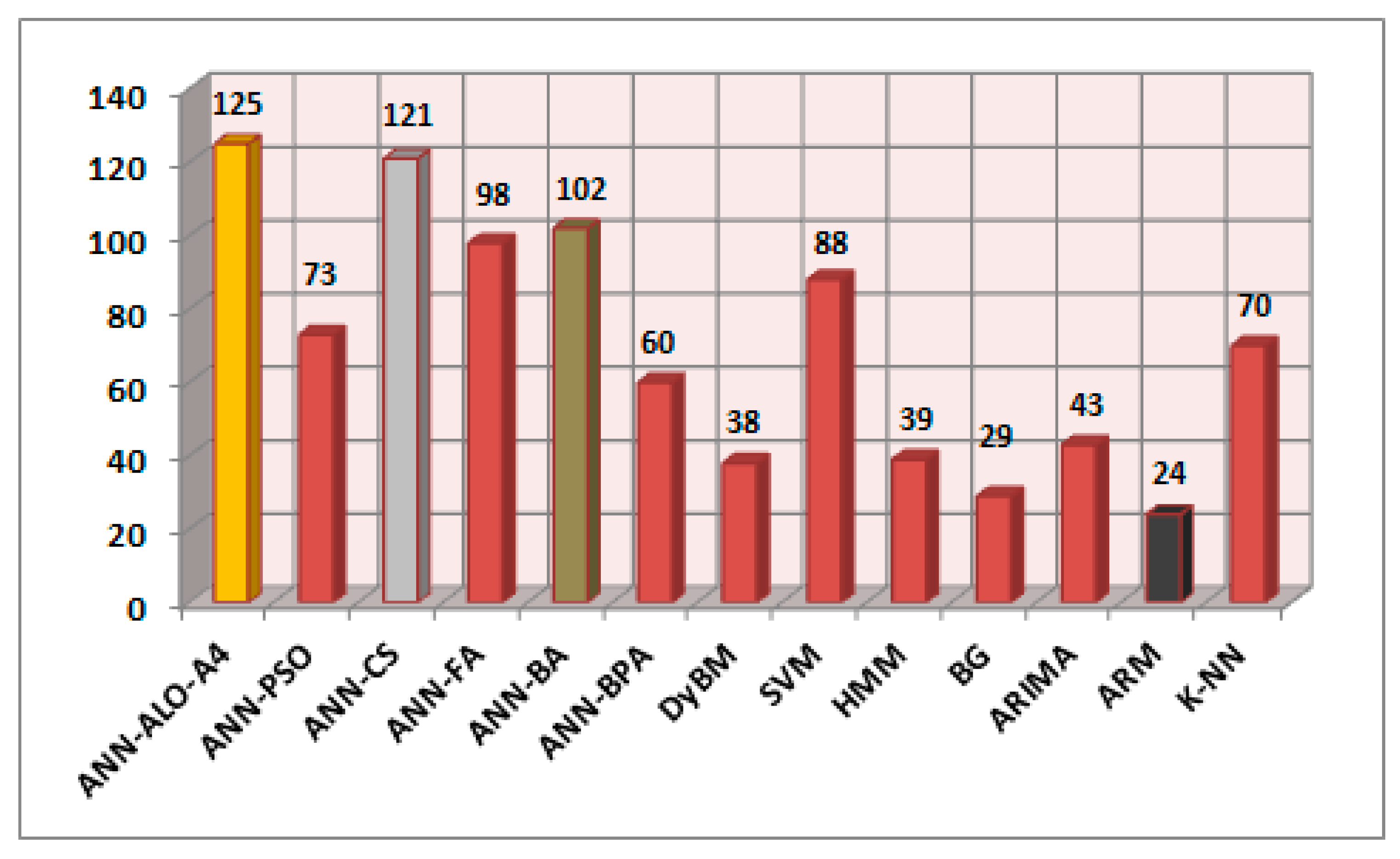
| Total Points | 125 | 73 | 121 | 98 | 102 | 60 | 38 |
| Application (EEG Time Series) | SVM | HMM | BG | ARIMA | ARM | K-NN |
|---|---|---|---|---|---|---|
| A1 | 2 (+12) | 6 (+8) | 12 (+2) | 10 (+4) | 13 (+1) | 4 (+10) |
| A2 | 8 (+6) | 7 (+7) | 11 (+3) | 10 (+4) | 13 (+1) | 9 (+5) |
| A3 | 8 (+6) | 13 (+1) | 10 (+4) | 9 (+5) | 12 (+2) | 7 (+7) |
| A4 | 7 (+7) | 12 (+2) | 11 (+3) | 8 (+6) | 9 (+5) | 10 (+4) |
| A5 | 3 (+11) | 10 (+4) | 9 (+5) | 12 (+2) | 13 (+1) | 4 (+10) |
| A6 | 3 (+11) | 10 (+4) | 12 (+2) | 11 (+3) | 13 (+1) | 8 (+6) |
| A7 | 5 (+9) | 12 (+2) | 13 (+1) | 11 (+3) | 10 (+4) | 6 (+8) |
| A8 | 8 (+6) | 11 (+3) | 10 (+4) | 6 (+8) | 12 (+2) | 7 (+7) |
| A9 | 5 (+9) | 7 (+7) | 11 (+3) | 13 (+1) | 10 (+4) | 6 (+8) |
| A10 | 3 (+11) | 13 (+1) | 12 (+2) | 7 (+7) | 11 (+3) | 9 (+5) |
| Total Points | 88 | 39 | 29 | 43 | 24 | 70 |
| Hospital | Physician | Usability | Accuracy | Speed | Effectiveness | Novelty |
|---|---|---|---|---|---|---|
| Isparta State Hospital | P1 | 5 | 5 | 4 | 5 | 5 |
| Isparta State Hospital | P2 | 4 | 5 | 3 | 4 | 4 |
| Hospital of Suleyman Demirel University (SDU) | P3 | 5 | 5 | 4 | 5 | 4 |
| Meddem Hospital | P4 | 4 | 4 | 5 | 5 | 4 |
| Meddem Hospital | P5 | 5 | 5 | 3 | 5 | 5 |
| Davraz Life Hospital | P6 | 5 | 4 | 4 | 4 | 4 |
| Mean | 4.67 | 4.67 | 3.83 | 4.67 | 4.33 |
© 2018 by the author. Licensee MDPI, Basel, Switzerland. This article is an open access article distributed under the terms and conditions of the Creative Commons Attribution (CC BY) license (http://creativecommons.org/licenses/by/4.0/).
Share and Cite
Kose, U. An Ant-Lion Optimizer-Trained Artificial Neural Network System for Chaotic Electroencephalogram (EEG) Prediction. Appl. Sci. 2018, 8, 1613. https://doi.org/10.3390/app8091613
Kose U. An Ant-Lion Optimizer-Trained Artificial Neural Network System for Chaotic Electroencephalogram (EEG) Prediction. Applied Sciences. 2018; 8(9):1613. https://doi.org/10.3390/app8091613
Chicago/Turabian StyleKose, Utku. 2018. "An Ant-Lion Optimizer-Trained Artificial Neural Network System for Chaotic Electroencephalogram (EEG) Prediction" Applied Sciences 8, no. 9: 1613. https://doi.org/10.3390/app8091613
APA StyleKose, U. (2018). An Ant-Lion Optimizer-Trained Artificial Neural Network System for Chaotic Electroencephalogram (EEG) Prediction. Applied Sciences, 8(9), 1613. https://doi.org/10.3390/app8091613