Vertical Seismic Profile Wavefield Separation Using Median Filtering Constrained by the Linear Radon Transform

Featured Application

The proposed wave separation method is applicable for the extraction of target wave mode in a borehole seismic survey. Particularly, when it is difficult to pick events manually for the mixed wavefields including downgoing and upgoing P-waves and S-waves, the proposed method can be employed to separate different wavefields automatically and accurately. In addition, in a processing of surface seismic data or raw dipole acoustic logging, this method also has application potential for the wave separation.

Abstract

Separation of downgoing and upgoing P-waves and S-waves in an offset 2D/3D vertical seismic profile (VSP) record is a basic step in VSP data processing. Radon transform and median filtering methods are commonly used to separate wavefields. However, with the former, it is hard to strike a balance between the resolution and amplitude preservation, while the latter ignores the variation in the slowness (apparent velocity) of events. In order to solve these problems, we propose a method based on a modified linear Radon transform and dynamic time shifting. We derive the slowness spectrum of an input VSP record through the modified Radon transform. Based on the optimal slope values of the events derived from the slowness spectrum, we align the wavefields by dynamic time shifting. Then, the target wavefields are separated using a median filtering constrained by the linear Radon transform. Our wavefield separation process is iterated until the four kinds of wavefields are separated according to a priority ranking based on the order of the energy spectrum from strong to weak. The results were found to be better than those derived from wave separation using the traditional median filter or those derived using the high-resolution Radon transform method.

1. Introduction

In a vertical seismic profile (VSP) recording, positive-slowness downgoing wavefields and negative-slowness upgoing wavefields interfere with each other [1]. An effective separation of original VSP data (common shot point gather) is essential before imaging, and separation represents one of the fundamental processing steps for VSP data [2]. Many methods exist that can be used successfully to separate wavefields propagating uniformly within a chosen analysis window [3,4,5,6].

The f–k (frequency–wave number) filtering method utilizes the difference of the slowness in the upgoing and downgoing waves for wavefield separation [7]. However, the overlap of the energy spectrum between different f–k quadrants can prevent these wavefields from being separated accurately [8]. Additionally, spatial samples are required to be sufficiently dense, otherwise the spatial alias frequency is generated. Glangeaud et al. [9] pointed out that for an f–k filter, a stable wavefield separation depends on the discrimination of different wavefields in the f–k domain. The Radon transform is a method of wavefield separation in the τ–p (intercept time–slowness) domain that utilizes the slowness of the upgoing and downgoing waves [10], and it can be implemented with either a linear Radon transform (also called the τ–p transform [11]) or a nonlinear Radon transform. Miao et al. [12] proved, through a case study, that the Radon transform wavefield separation technique is effective for separating the upgoing and downgoing waves, and application of a hyperbolic filter further improved the wavefield separation. Trad et al. [13] introduced the sparse constraint and proposed the high-resolution Radon transform method, which can be used to improve the accuracy of wavefield separation. Sacchi et al. [14] used an iterative double weighted conjugate gradient algorithm to solve nonlinear inversion problems of the high-resolution Radon transform. However, the resolution and AVO (amplitude versus offset) characteristics of common Radon transform methods are hard to retain [15].

The methods for wavefield separation with amplitude preservation include median filtering [16], mean filtering, and various other improved methods [17,18,19,20]. Among these methods, median filtering has been widely used for VSP wavefield separation because of the resulting low amplitude change and the stability in cases of short arrays. In order to effectively separate VSP downgoing and upgoing waves, Rao et al. [21] combined the τ−p domain masking filter, the median filter, and the f−k domain masking filter in a dynamic manner. Kommedal et al. [8] compared the median filter and other methods commonly used in the industry and showed how the median filter treated coherent and random noise; they also demonstrated that the median filter had a unique ability to preserve discontinuities and avoid smearing. Mars et al. [22] developed a new type of multichannel filter called a “constrained eigenvector filter”; this method can obtain better separation results than the median filters and eigenvector filters because it combines the advantages of the two approaches. In the application of these methods, seismic traces should be aligned according to the first arrival of the target wavefield [23]. Therefore, extensive first-break pickup work is inevitable and the events of a target wavefield can be aligned only if the first arrival is parallel to the other events of the target wavefield.

However, a different offset of the same wavefield will result in non-parallel events in the non-zero offset VSP [24,25]. Furthermore, the events of the same wavefield may come from different reflection layers and the reflection coefficients may be different, which will lead to changes in the slowness and the non-parallel events of the same wavefield. Therefore, a static time shift cannot exactly align the events of the target wavefield, thus resulting in a reduction of the wavefield separation accuracy.

In this paper, we propose a new median filtering method based on the constraint of the linear Radon transform to separate four kinds of wavefields whether or not the events in the wavefields are parallel. We first use a new superposition algorithm of the linear Radon transform to make the energy spectrum in the τ–p domain more focused than the traditional Radon transform so as to obtain the exact slowness value and variation of the slowness at different intercept times. Secondly, all the upgoing and downgoing P-waves and S-waves are aligned dynamically based on the variation characteristics of the wavefield slowness instead of just aligning the first arrivals in a routine VSP process. Lastly, we employ median filtering to separate four wavefields gradually according to the order of the energy spectrum from strong to weak.

2. Methods

2.1. Conventional Median Filter

Conventional median filters are widely used in VSP wavefield separation. We set the amplitude of geophone i at time t as $\mathrm{d}(t_i)$ and half the length of the median filtering window as k. The median filter is then derived as follows [26]:

$$\mathrm{M}(t_i)=\arg \min \{\mathrm{d}(t_{i-k }),\dots ,\mathrm{d}(t_{i+k})\},k\le \frac{\max (i)}{2},$$

(1)

Before use of the median filter, the target wavefield needs to be aligned by time shifting, which is applied through the first arrival:

$$\Delta t(i)=t(i)-t(1),$$

(2)

where $t(i)$ is the time of the first arrival at geophone i by the manual picking or automatic picking algorithm. However, there are four kinds of wavefields in the VSP wavefield, namely, the downgoing P-wave, downgoing S-wave, upgoing P-wave, and upgoing S-wave. Normally, the downgoing P-wave is easy to pick at first arrival, but the other three kinds of wavefields are difficult to pick because they are covered by the strong energy of the downward P-waves. Furthermore, the events of the same wavefield may come from different reflection layers and the reflection coefficient may be different, which will lead to changes in the slowness, and the events of the same wavefield will not be parallel as shown in Figure 1a. Even though the first arrival is picked accurately and aligned, the non-parallel events of the wavefield cannot be aligned through the same time shifting as shown in Figure 1b, which leads to a result in which the median filtering is incorrect. As shown in Figure 1c, there is an event (the black dashed arrow) that is missed in the result. Meanwhile, in the case of a low signal-to-noise ratio, the picking of the downgoing P-wave is affected by the noise, which leads to a result in which the events of the wavefield cannot be aligned, and this will reduce the accuracy of the results of the median filter. In order to obtain accurate time shifting and align all the events of the target wavefield, we calculated time shifting through the linear Radon transform as described in the following section.

2.2. Constraint under the Linear Radon Transform

When the seismic wave propagates to the geophone in the well, the slowness of the wavefield in the z direction is calculated by [27]:

$$p_n=\frac{\cos {\phi }_n }{v_n},$$

(3)

where ${\phi }_n$ is the angle between the direction of wave propagation and the z-axis (downward is positive), $v_n$ is the velocity of wave propagation, and $n$ is the type of wavefield. $p_n$ can also be considered the ray parameter of the wavefield events. When the length of the geophone array is much smaller than the depth of the geophones, the seismic wave can be regarded as a plane wave rather than a spherical wave. That means a direct wave or reflected wave from the same position reaches the geophones in a parallel direction. Therefore, the slowness of the wavefield is invariant with the geophones, and the events in the wavefield are approximately a straight line. The travel time of geophone level $i$ is:

$$t_i=t_1+\hspace{0.17em}i\Delta h{p}_n,$$

(4)

In the case of a short array, the reflection time–distance curves are approximately straight lines, and, therefore, the seismic wavefield in the space–time domain can be transformed into the τ–p domain by the linear Radon transform. The forward and inverse formulas of the sample angle stacking are [11,28,29]:

$$v(p,\tau )={\displaystyle \sum _{i=1 }^{N_x}u(h_i,t=\tau +h_{i}p)},$$

(5)

and

$$u(h_i,t)={\displaystyle \sum _{i=1 }^{N_x}v(p,\tau =t-h_{i}p)},$$

(6)

where $v(p,\tau )$ is the τ–p domain signal, t is the time, h is the depth, τ is the intercept time, p is the slowness, $u(h_i,t)$ is the inverse result, $N_x$ is the number of geophones, and $h_i$ is the depth of the number i geophone.

Different types of Radon forward transform can be used for wavefield separation. First, the seismic data in the space–time domain are transformed into the τ–p domain by Equation (5); after that, the wavefield is distinguished by the characteristics of different types of wavefields in the τ–p domain, and then the target wavefield is obtained by the Radon inverse transform shown in Equation (6). In addition to the linear Radon transform, there are a series of Radon transformations with different domains and different stack paths. In order to obtain the slowness values of the target wavefield, we only perform the Radon forward transformation without the Radon inverse transformation.

To increase the focus of the calculated energy spectrum in the τ–p domain, we add a time window to Equation (5) and improve it as:

$$V(p,\tau )={\displaystyle \sum _{m=-\frac{M}{2} }^{\frac{M}{2}}\frac{{\displaystyle \sum _{i=1}^{N_x}{u}^2(h_i,t=\tau +h_{i}p+m)}}{{{\sigma }_m}^2[u(h_i,t)]}},$$

(7)

where M is the length of the time window and ${{\sigma }_m}^2$ is the variance of the amplitude sequence in the stack path of the sampling point m. Therefore, the modified τ–p domain seismic data (slowness spectrum) obtained by Equation (7) can show the amplitude similarity and the magnitude of the seismic wave energy spectrum in the stack path corresponding to different intercept times and slowness. The extreme point on the slowness spectrum is an important basis for calculating the reasonable slowness of the target wavefield. In the area of the slowness spectrum corresponding to the target wavefield (such as the upgoing P-wave), the variation of the slowness with the intercept time is approximated to be linear because the short arrangement of geophones makes the slowness change rate of the same wavefield small. In order to obtain this linear relation, we search for the positions of the optimal energy spectrum value $V_i(p_i,{\tau }_i),(i=1,2,\dots )$ in the modified τ–p domain and fit them linearly $(p_i,{\tau }_i)$. Hence, this satisfies the following:

$$\{\begin{array}{l}{p}_{n\min }\le p_n(\tau )\le p_{n\max }\\ p_i=a_n+b_n{\tau }_i\end{array},$$

(8)

where $n$ is a type of wavefield that can be expressed as the upgoing or downgoing P-wave or S-wave. $p_{n\min }$ and $p_{n\max }$ represent the minimum and maximum slowness values, respectively, and the slowness range of different types of waves can be determined by the modified τ–p transform. $a_n$ and $b_n$ are linear parameters obtained by linear fitting using the least-squares method.

2.3. Dynamic Time Shifting

From Equations (3) and (4), we obtain the time shifting for different geophones:

$$\Delta t_i=t_i-t_1=(i-1)\Delta h{p}_n=(i-1)\Delta h\frac{\cos {\phi }_n }{v_n}.$$

(9)

From Equation (9), the variation of According to Equation (9), the time shift for a geophone is affected by the velocity of the seismic wave and the direction of wave arrival. The upgoing or downgoing waves contain reflected waves from different interfaces, even if they are of the same type (such as an upgoing P-wave), and their propagation directions are not completely consistent. As a result, the static time shift (traditional median filtering method) cannot accurately align the events. Thus, the method of dynamic time shifting is necessary.

the slowness of the target wavefield with the intercept time is obtained. Therefore, in the space–time domain, the time shift of different geophones at different intercept times is satisfied:

$$\Delta t_n(i,\tau )=(i-1)\Delta h{p}_n=(i-1)\Delta h(a_n+b_n\tau )=t_i-\tau ,$$

(10)

Equation (10) can be deduced by eliminating τ as follows:

$$\Delta t_n(t_i)=\frac{(i-1)\Delta h(a_n+b_n{t}_i) }{(i-1)\Delta h{b}_n+1},$$

(11)

which indicates that the time shift varies with different geophones and time. According to the variation of the slowness of the target wavefield, the seismic data are dynamically aligned by Equation (11), and the target wavefield is separated by the median filter with Equation (1).

2.4. Workflow for the Method

The separation process is shown in Figure 2. The black arrows represent the events of the target wavefield, which are not parallel in the original seismic data (a). In the first step, (b) is obtained from the original seismic data (a) by the dynamic time shift. The events of the target wavefield are not parallel in (a), but the events are parallel in (b) after the dynamic time shift. In the second step, the aligned target wavefield is obtained by the median filtering method, from (b) to (c). In the third step, the target wavefield is obtained by reverse alignment using the time shift of the first step, from (c) to (d). In the fourth step, the target wavefield (d) is subtracted from the original data (a), and the remaining wavefield (e) is obtained.

The complete steps of this method are shown in Figure 3. The original VSP common-shot gathers are transformed to the modified τ–p domain, and the slowness points corresponding to the optimal energy spectrum values in the target wavefield are fitted linearly. Then, according to the fitting results, the original wavefield is separated according to the steps of Figure 2, and as a result, the target wavefield and the remaining wavefield are obtained. One then repeats the above steps with the remaining wavefield as the original wavefield until the last residual wavefield no longer contains the regulate wavefield. We separated the target wavefields in turn according to the strength of the energy spectrum. In Figure 3, only the adopted median filtering is a routine VSP data processing approach. In general, the downgoing wave energy spectrum is stronger than that of the upgoing wave [21], and the P-wave energy spectrum is stronger than that of the S-wave. Hence, the downgoing P-wave energy spectrum is stronger than that of the upgoing S-wave. The energy spectrum difference between the P-wave and S-wave in field data is larger than that in synthetic data because of the attenuation. So, the upgoing P-wave energy spectrum is stronger than that of the downgoing S-wave in field data but not in synthetic data. Therefore, the synthetic records are separated in this order: downgoing P-wave, downgoing S-wave, upgoing P-wave, and upgoing S-wave; meanwhile, for the field data the order is as follows: downgoing P-wave, upgoing P-wave, downgoing S-wave, and upgoing S-wave.

3. Synthetic Data Test

We used synthetic VSP records of a horizontal layered model to test the separation effect of this new method. The parameters of model are listed in

Table 1. Parameters of model 1.

Layer	Thickness (m)	P-Wave Velocity (m s−1)	S-Wave Velocity (m s−1)	Density (kg m−3)
1	600	2800	1616.6	2255.0
2	400	3200	1847.5	2331.6
3	600	3900	2251.7	2449.8
4	400	4500	2598.1	2539.0

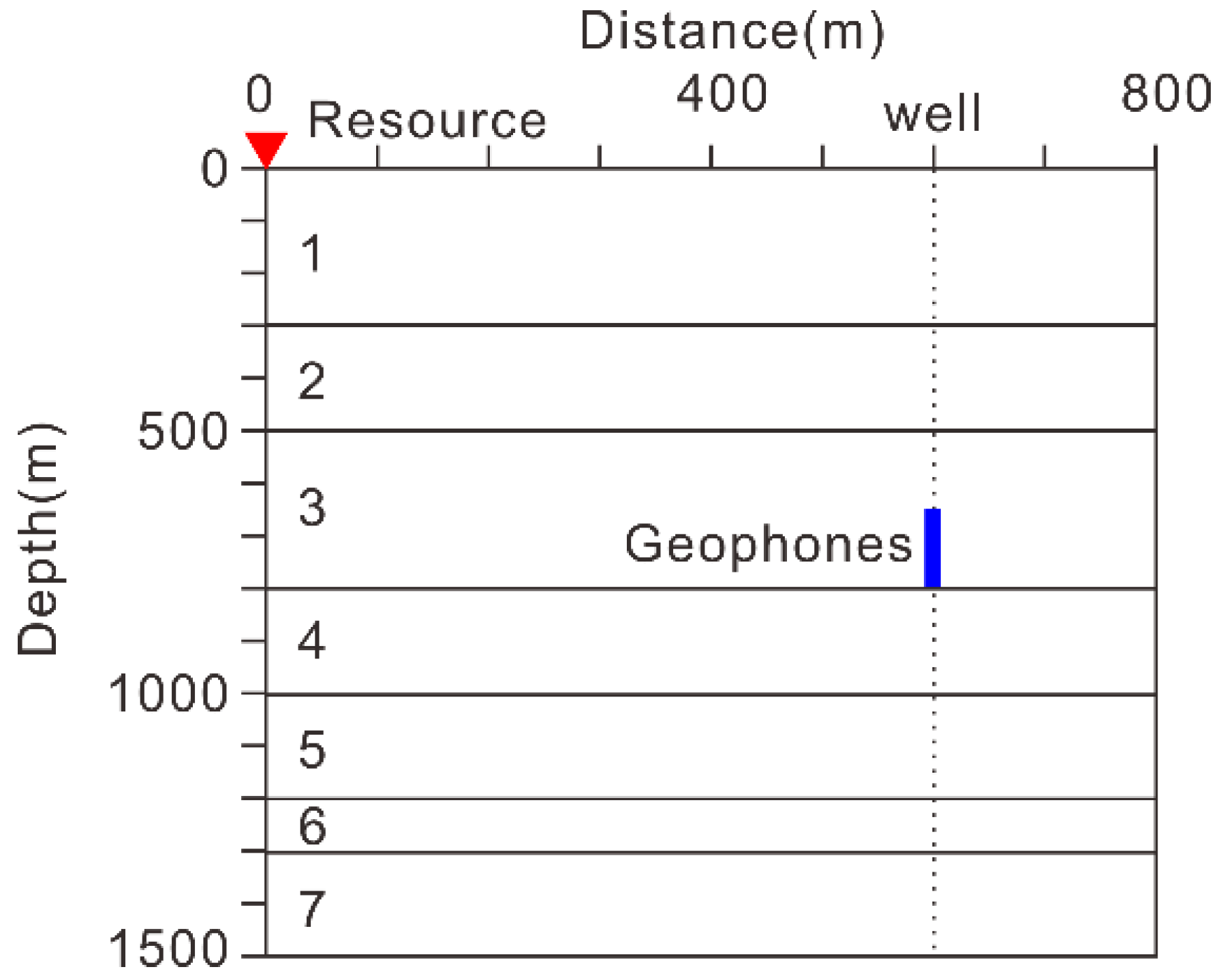
. The separation results were compared with the theoretical results and the results of the high-resolution Radon transform [13,30]. We set the wavelet as a Ricker wavelet with the peak frequency of 30 Hz, the initial phase was 0 degrees and it acts as an omni-directional point source. As shown in Figure 4, the geophones were located at the depth of 700–900 m with the interval of 5 m. The reflection coefficients were calculated through solving the Zoeppritz equations [31] at all the ray-paths derived using the ray-tracing method proposed by Levoy [32]. 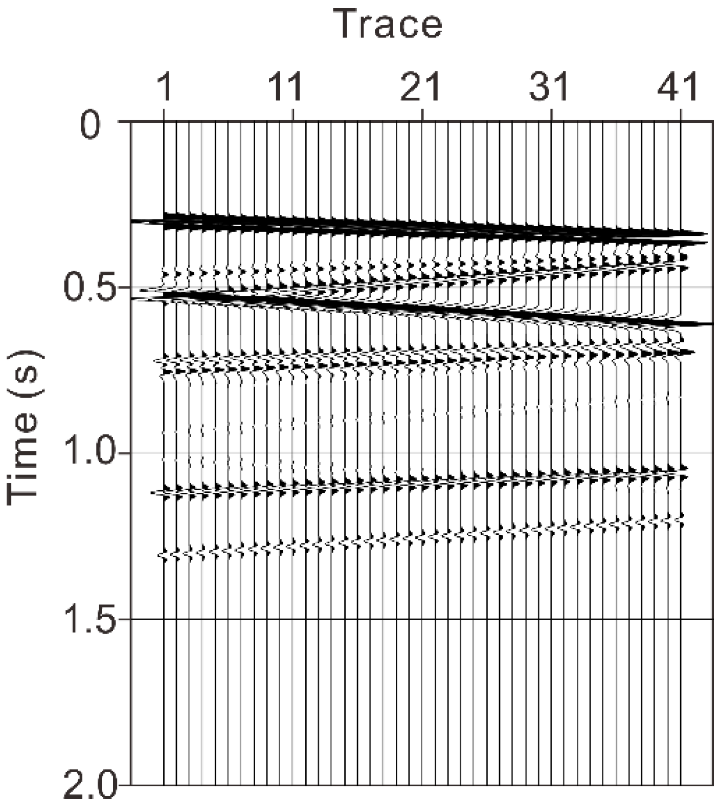Then, we synthesized the VSP record (Figure 5) through the convolution of the wavelet and calculated reflection coefficients. Figure 5 shows that the upgoing and downgoing P-waves and S-waves are mixed together. Because of the short array (the array length of the geophones was 200 m, which was 10% of the last layer depth), the events were approximately a straight line.

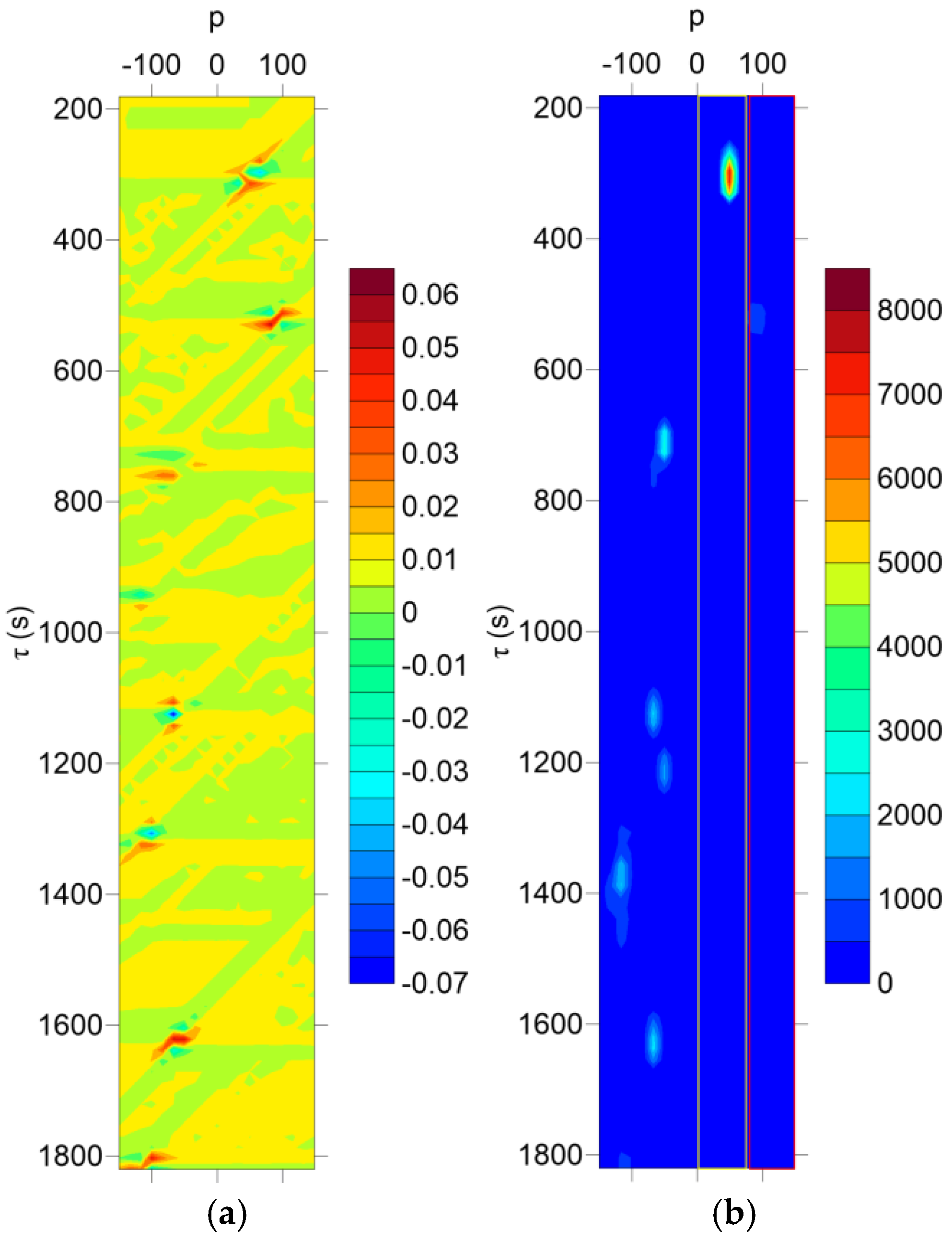
In order to compare the degree of energy spectrum focusing based on the conventional Radon transform and the modified Radon transform, we used Equations (5) and (7) to calculate the results of the two kinds of Radon transform, as shown in Figure 6. Figure 6a presents the results of the traditional linear Radon transform, and the local maximum and minimum points are given; notably, the energy spectrum was dispersive and similar to a “bow-tie” shape. Figure 6b shows the results of the modified Radon transform, and some local maximum points were in a vertical arrangement. Through a comparison of Figure 6a,b, we found that the energy spectrum of the modified Radon transform was more focused in the slowness direction, and the resolution was obviously improved, which allowed us to obtain a more accurate slowness.

The transform results in Figure 6b show that there were obvious differences in the slowness of the P-wave and S-wave events, and the energy spectra were distributed in different slowness regions. The yellow box in Figure 6b shows the region of the downgoing P-wave energy spectrum. By the linear fitting of the extremum points of this region, we can get $a=51$, $b=0$. According to Equations (11) and (12), the downgoing P-wave can be obtained by aligning and median filtering, as shown in Figure 7a. Similarly, by the linear fitting of the extremum points in the region of the S-wave in the red box, we get $a=89$, $b=0$. The downgoing S-wave can be obtained through Equation (10), as shown in Figure 7d. The downgoing P-wave and S-wave had only one event, which led to $b=0$ after linear fitting of the slowness, which means that the dynamic time shift became static. At the same time, the high-resolution Radon transform was used to separate the downgoing P-wave and S-wave from the original VSP data, as shown in Figure 7b,e. To verify the separation results, we synthesized the downgoing P-wave and S-wave, as shown in Figure 7c,f. The travel time, phase, and amplitude of the downgoing P-wave and S-wave were consistent with the theoretical results as determined through the comparison of the theoretical results with those from our method and the high-resolution Radon transform method.

After separating the downgoing P-wave and S-wave, we used Equation (5) to perform the linear Radon transform for the remaining wavefield, and we used Equation (7) to carry out the modified Radon transform. The results are shown in Figure 8. Similar to Figure 6, Figure 8 shows the energy spectrum divergence in a bow-tie shape, and the energy spectrum of the modified Radon transform was more focused in the slowness direction; the resolution was obviously improved, and so a more accurate slowness could be obtained. Based on Equation (5), the spectral values in Figure 8a are the superposition values of amplitudes along a straight line. However, based on Equation (7), they are the ratios of the superposition amplitudes to the variance of the amplitudes along a stack path. When the amplitudes along a certain stack path are similar, the variance value is close to zero. Thus, compared with the traditional τ–p transform, we can get more discriminative spectral values in Figure 8b, which are then employed to constrain the median filtering.

In the results of the modified Radon transform (Figure 8b), the yellow box shows the region of the upgoing P-wave energy spectrum. By the linear fitting of the extremum points of this region, we can get $a=-53.3$, $b=0.0088$. According to Equations (11) and (12), the upgoing P-wave can be obtained by aligning and median filtering, as shown in Figure 9a. Similarly, by the linear fitting of the extremum points in the region of the S-wave in the red box, we get $a=89$, $b=0.003$. The upgoing S-wave was obtained through Equation (10) and is shown in Figure 9d.

In order to further test the performance of the proposed method, we adopted a VSP record with more complicated wave interference. The parameters of model 2 are listed in

Table 2. Parameters of model 2.

Layer	Thickness (m)	P-Wave Velocity (m s−1)	S-Wave Velocity (m s−1)	Density (kg m−3)
1	300	2000	1150	2010
2	200	2200	1270	2100
3	300	2300	1330	2200
4	200	2400	1390	2400
5	200	2800	1618	2450
6	100	2300	1330	2350
7	200	3200	1846	2550

. As shown in Figure 10, the distance between the source and well is 600 m. The geophones are located at the depth of 600–795 m with an interval of 5 m. In the modelling, we applied the staggered-grid finite difference simulation. The peak frequency of Ricker wavelet was set as 50 Hz. As shown in Figure 11, the synthesized record presents more reflections and multiples, which intersect and interfere with each other.

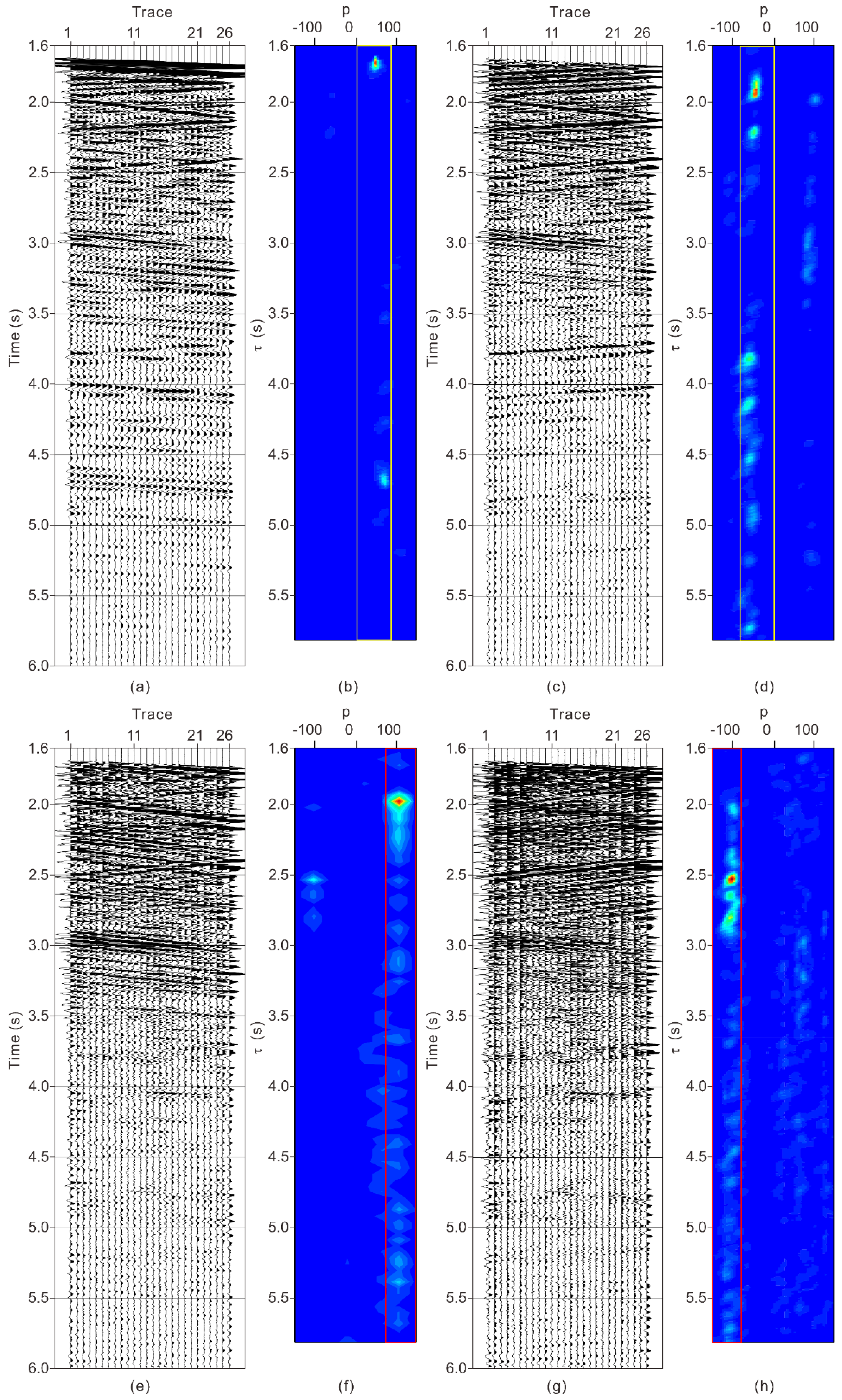
Our separation results (Figure 12a–d) were compared with the results of the high-resolution Radon transform (Figure 12e–h). They are displayed with the same gain parameters. It can be seen in Figure 12f that in the vicinity of 0.8 s, there are a few mixed upgoing wavefield events marked by the green arrow. Figure 12f,h contain the weak P-wave first arrivals marked by the blue arrows. As shown in Figure 11, there are two parallel events over 1.6 s indicated by the red arrows, which are both upgoing P-waves. In our method, they are well separated and shown in Figure 12c and marked by the red arrows. However, the high-resolution Radon transform method cannot well separate these events as shown by the red arrows shown in Figure 12g,h.

4. Field Data Application Results and Discussion

In order to test the application effect of this method, we used the original VSP data of the Z component in the Tuoputai area, Tarim Basin. The geophones were located from 3500 m (level 1) to 3750 m (level 26) in the TP327CH well at a spacing of 10 m. The target layer was located at the Middle Ordovician Yijianfang Formation (O2yj) at 6807–7378 m in the well. The reservoir space was mainly composed of fractures and pores with large scales and general connectivity. The reservoir lithology was dominated by pelsparite. The depth of the target layer was deeper than that of the geophones, and so the separation and imaging of the deep wavefield in the seismic records was very important for reservoir predictions.

Figure 13a illustrates one of the common shot point gathers. In the seismic records, the upgoing and downgoing waves were mixed with each other. First, the modified Radon transform was performed using Equation (7), and the results are shown in Figure 13b. Because the downgoing P-wave energy spectrum was the strongest, the region in the yellow box of Figure 13b could be preliminarily determined as the P-wave energy spectrum. By linear fitting the position of the extreme point in the region of the longitudinal wave energy spectrum, we get $a=37.48$, $b=0.0075$. According to Equations (11) and (12), the downgoing P-wave can be obtained by aligning and median filtering, and the results are shown in Figure 14b. The residual wavefield is shown in Figure 13c, and the modified Radon transform results are shown in Figure 13d. The red box area of Figure 13d was negative, which was determined as the upgoing P-wave, and after fitting the extreme value points, $a=-36.91$, $b=-0.01089$ were obtained. According to Equations (11) and (12), the upgoing P-wave can be obtained, and the results are shown in Figure 14c. Analogously, the residual wavefields (Figure 13e,g) and their modified Radon transform results (Figure 13f,h) were obtained. The upgoing P-wave (Figure 14d) and the upgoing S-wave (Figure 14e) were obtained by fitting the slowness points and median filtering. Figure 14a illustrates original VSP data. Comparing the separation results (Figure 14b,e) with the original data (Figure 14a), it is clear that there is not any wavefield interference in the separated upgoing and downgoing P-waves and S-waves from the proposed method. From Figure 14f, we can see that the residuals from the wavefield separation are mainly noise.

In the process of wavefield separation, the upgoing and downgoing waves can be easily distinguished by the positive and negative slowness. The key is in how to distinguish the P-wave and S-wave. Equation (1) shows that the slowness is determined by the direction and velocity of wave propagation. The S-wave has a smaller projection angle, reflection angle, and velocity than the P-wave, which makes the absolute slowness value of the S-wave greater than that of the P-wave. For the same type of wavefield, the angle φ may be changed, and so it should not be ignored for the accuracy of the separation results. However, the variation of cosφ is much smaller than the velocity difference between the P-wave and S-wave. Therefore, the energy spectra of the P-wave and S-wave on the slowness spectra can be separated.

For comparing Figure 14a,c, the downgoing P-wave including the first arrival of the P-wave was subtracted. The energy spectrum positions in the yellow box in Figure 14b correspond to the events of the downgoing P-wave in Figure 14a. By comparing Figure 14b,d, one can see that the upgoing P-wave energy spectrum of the remaining wavefield appeared after subtraction of the downgoing P-wave. After separating the upgoing P-wave from Figure 14c, the residual wavefield was obtained as shown in Figure 14e. The comparison between Figure 14d,f shows that when all the P-wave data were subtracted, the energy spectrum of the downgoing S-wave appeared, as shown in the red box of Figure 14f. Then, the downgoing S-wave was subtracted from Figure 14e and the energy spectrum of the upgoing S-wave appeared (Figure 14h). In the above process, the wavefields were subtracted in the order of the energy spectrum from strong to weak (downgoing P-wave, upgoing P-wave, downgoing S-wave, upgoing S-wave). With this process, after the former wavefield is subtracted, the energy spectrum of the later wavefield appears.

In order to verify the accuracy of the results, the methods of high-resolution Radon transform and static time shifting (traditional median filtering) were used to separate the original data. We compared the separation results for our method with the high-resolution Radon transform method and static time-shift separation results at 5000–6000 ms, as shown in Figure 15. The contrast indicated that parts of the events of the deep reflection wave were broken by the static time-shift median filtering method, which was obviously due to the inaccuracy of the slowness value that resulted in the misalignment of events. However, the median filtering method based on dynamic alignment, because the event is aligned according to the actual accurate slowness value, basically did not reproduce the event faults. The results of the high-resolution Radon transform showed better continuity for some local events, but this method destroyed the variation of the amplitude and presented characteristic bifurcation patterns.

As shown in Figure 16, we compared the residuals of the three methods to analyze whether there is important energy left. In the red and green quadrilaterals, there are several obvious downgoing wave events in Figure 16d but not in Figure 16b,c. In addition, the blue quadrilaterals in Figure 16c show a weak downgoing wave event but there are no events left in the corresponding position in Figure 16b. Besides, the slowness spectrum of residual wavefield using our method is the weakest of Figure 16i–k. This indicates that the effective energy left in residual wavefield using our method is less than those of other methods.

In the slowness spectrum, the upgoing and downgoing waves can be distinguished according to the positive or negative characteristics of the slowness with the proposed method. The P-waves and S-waves can be distinguished by the magnitude of the absolute value of the slowness because of the differences in the velocity and incidence angle. According to the results of this study, although the slowness of the same wavefield was variable with the intercept time, the quantity of the variation was not enough to exceed the slowness difference between the P-wave and S-wave, and so in the slowness spectrum, the P-wave and S-wave could be distinguished. Because of the differences in the energy spectrum between different wavefields, the four wavefields were separated successfully according to the priority ranking based on the order of the energy spectrum from strong to weak.

Our method is suitable for VSP data with short arrays, and it is based on the assumption of straight events and linear variation of slowness. For long arrays or complex strata, data could be decomposed into several short array datasets, which is an approach that will be assessed in future research. Because we separate the wavefields in common-shot gather using our method, it is applicable for 2D and 3D offset-VSP data. In regard to the results derived with this method, there were some errors encountered in approaching the first and the last trace. In general, less geophones for VSP data will result in larger ratios of the error trace, which is caused by the systematic error of median filtering. The median filtering can be replaced by mean filtering and singular value decomposition (SVD), and the application effect will be realized in future research.

5. Conclusions

We proposed a new method for VSP separation based on median filtering constrained by the linear Radon transform. This method combines the slowness calculation of the linear Radon transform and the amplitude preserving feature of the median filter and thus retains the advantages of both methods. We used the modified Radon transform to determine the exact slowness values of the target wavefields as a constraint. In the process of aligning the wavefield, the time shift of the wavefield was not equal to that of the first arrival, and so we used a method involving a dynamic time shift. Because of the differences in the energy spectrum for different wavefields, we did not separate the four wavefields at one time; instead, we separated them according to a priority ranking based on the order of the energy spectrum from strong to weak. The comparisons between the results of different approaches showed that our separation method is effective for both numerical and field data applications, and that the effect of the proposed method is better than that of the traditional median filter and the high-resolution Radon transform. This method will be efficacious for obtaining pure wavefields in VSP seismic surveys.

References

1. Hardage, B.A. Vertical Seismic Profiling: Principles, 3rd Updated and Revised ed.; Seismic Exploration 14, Pergamon; Elsevier Science: New York, NY, USA, 2000; pp. 154–174. [Google Scholar]
2. Gao, L.; Chen, W.C.; Wang, B.L. VSP wave field separation: An optimization method based on block relaxation and singular value thresholding. J. Appl. Geophys. 2014, 104, 156–162. [Google Scholar] [CrossRef]
3. Aminzadeh, F. A recursive method for the separation of upgoing and downgoing waves of vertical seismic profiling data. Geophysics 1986, 5, 2206–2218. [Google Scholar] [CrossRef]
4. Seeman, B.; Horowicz, L. Vertical seismic profiling: Separation of upgoing and downgoing acoustic waves in a stratified medium. Geophysics 1983, 48, 555–568. [Google Scholar] [CrossRef]
5. Simaan, M. Optimum array filters for array data signal processing. IEEE Trans. Acoust. Speech Signal Process. 1983, 31, 1006–1015. [Google Scholar] [CrossRef]
6. Simaan, M.; Love, P. Optimum suppression of coherent signals with linear moveout in seismic data. Geophysics 1984, 49, 215–226. [Google Scholar] [CrossRef]
7. Christie, P.A.F.; Hughes, V.J.; Kennett, B.L.N. Velocity filtering of seismic reflection data. First Break 1983, 1, 9–24. [Google Scholar] [CrossRef]
8. Kommedal, J.H.; Tjøstheim, B.A. A study of different methods of wavefield separation for application to VSP data. Geophys. Prospect. 1989, 2, 117–142. [Google Scholar] [CrossRef]
9. Glangeaud, F.; Mari, J.L. Wave separation. Part two: Applications La séparation des ondes. Deuxième partie: Applications. Oil Gas Sci. Technol. 2006, 1, 21–61. [Google Scholar]
10. Moon, W.; Carswell, A.; Tang, R.; Dilliston, C. Radon transform wave field separation for vertical seismic profiling data. Geophysics 1986, 51, 940–947. [Google Scholar] [CrossRef]
11. Carswell, A.; Tang, R.; Dillistone, C.; Moon, W. A new method of field separation in VSP data processing. In Proceedings of the 54th Annual SEG Meeting, Atlanta, GA, USA, 6–7 December 1984; pp. 40–42. [Google Scholar] [CrossRef]
12. Miao, X.G.; Moon, W.M.; Milkereit, B. A multioffset, three-component VSP study in the Sudbury Basin. Geophysics 1995, 60, 341–353. [Google Scholar] [CrossRef]
13. Trad, D.Q.; Ulrych, T.J.; Sacchi, M.D. Accurate interpolation with high-resolution time-variant Radon transforms. Geophysics 2002, 67, 644–656. [Google Scholar] [CrossRef]
14. Sacchi, M.D.; Porsani, M. Fast high-resolution parabolic Radon transform. In Proceedings of the 69th Annual SEG Meeting, Houston, TX, USA, 31 October–5 November 1999; pp. 1477–1480. [Google Scholar] [CrossRef]
15. Schonewile, M.; Zwartjes, P. High-resolution transforms and amplitude preservation. In Proceedings of the 72th Annual SEG Meeting, Denver, CO, USA, 14–16 April 2002; pp. 2066–2069. [Google Scholar] [CrossRef]
16. Stewart, R.R. Median filtering: Review and a new f/k analogue design. J. Can. Soc. Explor. Geophys. 1985, 1, 54–63. [Google Scholar]
17. Duncan, G.; Beresford, G. Attentuation of coherent noise using automatic direction median filtering. Explor. Geophys. 1992, 2, 127–132. [Google Scholar] [CrossRef]
18. Duncan, G.; Beresford, G. Median filter behavior with seismic data. Geophys. Prospect. 1995, 43, 329–345. [Google Scholar] [CrossRef]
19. Gao, L.; Chen, W.C.; Wang, B.L.; Gao, J.H. Zero-offset VSP wavefield separation using two-step SVD approach. Chin. J. Geophys. Chin. Ed. 2013, 5, 1667–1675. [Google Scholar]
20. Wang, X.K.; Chen, J.Y.; Gao, L.; Chen, W.C. An iterative zero-offset VSP wavefield separating method based on the error analysis of SVD filtering. IEEE Geosci. Remote Sens. Lett. 2018, 15, 1164–1168. [Google Scholar] [CrossRef]
21. Rao, Y.; Wang, Y.H. VSP wave separation by adaptive masking filters. J. Geophys. Eng. 2016, 13, 412–421. [Google Scholar] [CrossRef] [Green Version]
22. Mars, J.; Rector, J.W.; Lazaratos, S.K. Filter formulation and wavefield separation of cross-well seismic data. Geophys. Prospect. 1999, 5, 611–636. [Google Scholar] [CrossRef]
23. Blias, E. Multi-criteria approach to automatic first arrival picking for 3C 3D VSP data. In Proceedings of the 80th Annual SEG Meeting, Denver, CO, USA, 21–25 October 2010; pp. 4314–4318. [Google Scholar] [CrossRef]
24. Blias, E. VSP wavefield separation: Wave-by-wave approach. In Proceedings of the 75th Annual SEG Meeting, Houston, TX, USA, 7–11 November 2005; pp. 2609–2612. [Google Scholar] [CrossRef]
25. Blias, E. VSP wavefield separation: Wave-by-wave optimization approach. Geophysics 2007, 4, T47–T55. [Google Scholar] [CrossRef]
26. Lu, J.; Wang, Y.; Chen, J.Y. Noise attenuation based on wave vector characteristics. Appl. Sci. 2018, 8, 672. [Google Scholar] [CrossRef]
27. Jovanovic, K.; Marfurt, K.J. P and S waves separation from vector VSP’s by a blocky antialias Discrete Radon Transform: Application to Vinton Dome, LA. In Proceedings of the 74th Annual SEG Meeting, Denver, CO, USA, 10–15 October 2004; pp. 2513–2516. [Google Scholar] [CrossRef]
28. Beylkin, G. Discrete Radon transform. IEEE Trans. Acoust. Speech. Signal Process. 1987, 35, 162–172. [Google Scholar] [CrossRef]
29. Lun, D.P.K.; Hsung, T.C.; Siu, W.C. On the convolution property of a new discrete Radon transform and its efficient inversion algorithm. In Proceedings of the ISCAS’95—International Symposium on Circuits and Systems, Seattle, WA, USA, 30 April–3 May 1995; pp. 1892–1895. [Google Scholar]
30. Sacchi, M.D.; Ulrych, T.J. Model re-weighted least-squares Radon operators. SEG Tech. Program Expand. Abstr. 1995, 14, 616–618. [Google Scholar] [CrossRef]
31. Aki, K.; Richard, P.G. Quantitative Seismology, Theory and Methods, 2nd ed.; Freeman: San Francisco, CA, USA, 1980. [Google Scholar]
32. Levoy, M. Efficient ray tracing of volume data. ACM Trans. Graph. 1990, 9, 245–261. [Google Scholar] [CrossRef] [Green Version]
Figure 1. The process of separating a single wavefield using the conventional median filter in the case of non-parallel events in the target wavefield. Δt represents the masximum time shift of the first arrival; black arrows denote downgoing P-wave events, red arrows denote downgoing S-wave events, green arrows denote upgoing S-wave events, and blue arrows denote upgoing S-wave events. (a) Original seismic data; (b) Statically aligned data; (c) Target wavefield after median filtering.
Applsci 08 01494 g001
Figure 2. The process of separating a single wavefield using the new method. Black arrows denote downgoing P-wave events, red arrows denote downgoing S-wave events, green arrows denote upgoing S-wave events, and blue arrows denote upgoing S-wave events. (a) Original seismic data; (b) Dynamic aligned data; (c) Target wavefield after median filtering; (d) Target wavefield; (e) The remaining wavefield.
Applsci 08 01494 g002
Figure 3. Flowchart of separation for the vertical seismic profile (VSP) wavefield.
Applsci 08 01494 g003
Figure 4. Sketch map of model 1. The red triangle is the resource and the blue line is the sequence of the geophones.
Applsci 08 01494 g004
Figure 5. Synthetic VSP record based on model 1.
Applsci 08 01494 g005
Figure 6. The results for the (a) traditional and (b) modified linear Radon transform based on the synthetic VSP records.
Applsci 08 01494 g006
Figure 7. Results for the downgoing wavefield and theoretical wavefield. (a) Downgoing P-wave obtained by our method; (b) Downgoing P-wave obtained by the high-resolution Radon transform; (c) Theoretical downgoing P-wave; (d) Downgoing S-wave obtained by our method; (e) Downgoing S-wave obtained by the high-resolution Radon transform; (f) Theoretical downgoing S-wave.
Applsci 08 01494 g007
Figure 8. The results for the (a) traditional and (b) modified linear Radon transform based on the VSP data after subtraction of the downgoing wavefields in the original synthetic VSP records.
Applsci 08 01494 g008
Figure 9. Results for the upgoing wavefield and theoretical wavefield. (a) Upgoing P-wave obtained by our method; (b) Upgoing P-wave obtained by the high-resolution Radon transform; (c) Theoretical upgoing P-wave; (d) Upgoing S-wave obtained by our method; (e) Upgoing S-wave obtained by the high-resolution Radon transform; (f) Theoretical upgoing S-wave.
Applsci 08 01494 g009
Figure 10. Sketch map of model 2. The red triangle is the resource and the blue line is the sequence of the geophones.
Applsci 08 01494 g010
Figure 11. Synthetic VSP record based on model 2.
Applsci 08 01494 g011
Figure 12. Results for the separation of the VSP wavefield. (a,e) Downgoing P-wave; (b,f) Downgoing S-wave; (c,g) Upgoing P-wave; (d,h) Upgoing S-wave; (ad) Results for our method; (eh) Results for the high-resolution Radon transform method.
Applsci 08 01494 g012
Figure 13. Wavefield data after successive wave separations and the slowness spectrum. (a) Original VSP data; (b) Slowness spectrum of (a); (c) Residual wavefield after subtraction of the downgoing P-wave in (a); (d) Slowness spectrum of (c); (e) Residual wavefield after subtraction of the upgoing P-wave in (c); (f) Slowness spectrum of (e); (g) Residual wavefield after subtraction of the downgoing S-wave in (e); (h) Slowness spectrum of (g).
Applsci 08 01494 g013
Figure 14. Results for the separation of the VSP wavefield. (a) Original VSP data; (b) Downgoing P-wave; (c) Downgoing S-wave; (d) Upgoing P-wave; (e) Upgoing S-wave; (f) Residual wavefield after subtraction of four wavefields.
Applsci 08 01494 g014
Figure 15. Results for the separation of the VSP wavefield. (a,e,i) Downgoing P-wave; (b,f,j) Downgoing S-wave; (c,g,k) Upgoing P-wave; (d,h,l) Upgoing S-wave; (ad) Results for our method; (eh) Results for traditional median filtering; (il) Results for the high-resolution Radon transform method.
Applsci 08 01494 g015
Figure 16. Residual wavefield after subtraction of four wavefields. (a) Original VSP data; (b) Residual wavefield using our method; (c) Residual wavefield using traditional median filtering; (d) Residual wavefield using the high-resolution Radon transform; (eh) are zoomed versions of (ad), respectively; (i) Slowness spectrum of (b); (j) Slowness spectrum of (c); (k) Slowness spectrum of (d).
Applsci 08 01494 g016