A Software Reliability Model Considering the Syntax Error in Uncertainty Environment, Optimal Release Time, and Sensitivity Analysis

Abstract

The goal set by software developers is to develop high quality and reliable software products. During the past decades, software has become complex, and thus, it is difficult to develop stable software products. Software failures often cause serious social or economic losses, and therefore, software reliability is considered important. Software reliability growth models (SRGMs) have been used to estimate software reliability. In this work, we introduce a new software reliability model and compare it with several non-homogeneous Poisson process (NHPP) models. In addition, we compare the goodness of fit for existing SRGMs using actual data sets based on eight criteria. The results allow us to determine which model is optimal.

1. Introduction

The basic goal set by software developers is to develop high quality software products that are stable and reliable. As technology has advanced, consumers demand more functions. For this reason, the software structure has become more complex during the last few decades, which makes it difficult to produce software with high quality and stable reliability [1]. Software reliability growth models (SRGMs) have been used by researchers to estimate software reliability. The goodness of fit is decided by common criteria, which will be discussed in Section 3. Many SRGMs have been developed during the past decades. Most SRGMs are based on a non-homogeneous Poisson process (NHPP). These models assume that the total number of failures follows $\mathrm{m}\left(\mathrm{t}\right)$, which is a mean value function based on a NHPP. SRGMs are distinguished by its unique function, $\mathrm{m}\left(\mathrm{t}\right)$. This $\mathrm{m}\left(\mathrm{t}\right)$ reflects various environments through the assumptions of the parameters. After developing a software reliability model, we fit the model to the actual data and estimate its goodness of fit. If the model that best fits the actual data is determined, it is possible to estimate the optimal release time and the minimum expected cost of development, thereby establishing a release policy. Thus, it is crucial to consider not only the development of a model that reflects diverse environmental factors but also one that presents the best goodness of fit for actual data sets.

Goel–Okumoto [2] developed an exponential model that has been extended to develop SRGMs as a basic framework. Yamada [3,4] proposed the inflection S-shaped NHPP model and the delayed S-shaped NHPP model, which incorporates the testing effort. Quadri et al. [5] and Ahmad et al. [6] extended the SRGM with the exponentiated Weibull to consider testing efforts. Pham et al. [7] proposed the Pham–Zhang Model that has the Inflection S-shaped model as fault detection function. Pham and Zhang [8] proposed a generalized NHPP software testing coverage model. Several studies have focused on the factors of the development environment. Teng et al. [9] dealt with software reliability models with parameters that indicated the random field environments. Pham [10] discussed a new model that incorporates the uncertainty of the system fault detection rate per unit of time subjected to operating environments. Inoue et al. [11] conducted software reliability modeling considering the uncertainty of the testing environment. Li et al. [12] performed new testing coverage modeling that considers not only the error generation but also the fault removal efficiency based on NHPP. Song et al. [13,14,15] considered operating environments. They applied random variable to the software reliability model, which represent the uncertainty in the operating environment. Zhu et al. [16] defined two type of software faults for considering software fault dependency and imperfect fault removal. Zhu et al. [17] described a theoretic software reliability model follows gamma distribution incorporating the fault detection process is a stochastic process due to the randomness caused by the environmental factors. As shown above, many software reliability models have been proposed. In addition, several papers have been suggested from the statistical method perspective. Zeephongsekul et al. [18] applied the maximum-likelihood estimation of parameters. Candini et al. [19] referred to a Bayesian Monte Carlo method to estimate small failure probabilities with uncertainties. Meta learning and deep learning have been brought to attention recently. Caiuta et al. [20] applied meta-learning algorithms in software reliability models. Tamura et al. [21] performed simulations to select the optimal software reliability model based on deep learning. Tamura et al. [22] and Wang et al. [23] studied the prediction of the number of software failures based on a deep learning model. Kim et al. [24] explained application of the software reliability model to increase the software reliability, and introduced not only some analytical methods but also the prediction and estimation results.

In this paper, we propose a new NHPP SRGM based on the Weibull distribution, which considers testing time with syntax error. Then, we discuss optimal release time and sensitivity analysis using the proposed model. In Section 2, the proposed model mean value function with common NHPP SRGMs is presented. We show eight criteria to estimate the goodness of fit in Section 3. Section 4 discusses the best model by various criteria using actual data sets. Section 5 examines software release policy and Section 6 deals with sensitivity analysis of parameters affecting the release policy. Finally, conclusions are presented in Section 7 and future research topics are suggested in Section 8.

2. Proposed Software Reliability Model

2.1. Non Homogeneous Poisson Process Model

General software reliability models follow the NHPP as follows;

$$\mathrm{Pr}\left\{\mathrm{N}\left(\mathrm{t}\right)=\mathrm{n}\right\}=\frac{{\left[\mathrm{m}\left(\mathrm{t}\right)\right]}^{\mathrm{n}}}{\mathrm{n}!}{\mathrm{e}}^{-\mathrm{m}\left(\mathrm{t}\right)},\mathrm{n}=0,1,2,\dots .$$

(1)

where m(t) is mean value function, which is expected number of failures detected by testing time t.

It can be written as:

$$\mathrm{m}\left(\mathrm{t}\right)={\int }_0^{\mathrm{t}}\mathsf{\lambda }\left(\mathrm{s}\right)\mathrm{ds}$$

(2)

where $\mathsf{\lambda }\left(\mathrm{t}\right)$ is intensity function of failure.

Most of NHPP SRGM is expressed using the differential equation as:

$$\frac{\mathrm{dm}\left(\mathrm{t}\right)}{\mathrm{dt}}=\mathrm{b}\left(\mathrm{t}\right)\left[\mathrm{a}\left(\mathrm{t}\right)-\mathrm{m}\left(\mathrm{t}\right)\right]$$

(3)

Through solution of Equation (3), that make to find unique m(t) using $\mathrm{a}\left(\mathrm{t}\right)$ and $\mathrm{b}\left(\mathrm{t}\right)$. Also, this process can be applied to assume for software testing.

2.2. Proposed Software Reliability Model

The proposed model is also based on the NHPP. The mean value functions of the proposed model and the testing coverage model are similar, but there are some differences.

The important point is the proposed model consider uncertainty environment. The actual testing environment and the theoretical test environment of the software are very different. In an actual testing environment, the developer may have unexpected variables like syntax error, which is considered in proposed model.

Figure 1 shows infrastructure of time testing. Generalized testing time of the SRGMs is 0 < t. However, if the software that will perform the test has a syntax error, it cannot be compiled and tested. To continue testing it, the code must be modified to remove the syntax errors. Thus, the actual testing time differs from the theoretical testing time. This is a point that the proposed model considered. Testing time of proposed model considers the syntax error, which is an error in the syntax or tokens written in a programming language. So, the testing time of proposed model is ${\mathrm{t}}_0<\mathrm{t}$.

The mean value function $\mathrm{m}\left(\mathrm{t}\right)$ of the proposed model is based on the Weibull distribution model [14], which is the expected number of software failures by time $\mathrm{t}$ and is defined as follows:

$$\frac{\mathrm{dm}\left(\mathrm{t}\right)}{\mathrm{dt}}=\mathsf{\eta }\left[\mathrm{b}\left(\mathrm{t}\right)\right]\left[\mathrm{N}-\mathrm{m}\left(\mathrm{t}\right)\right]$$

(4)

where $\mathrm{b}\left(\mathrm{t}\right)$ is the failure detection rate function, $\mathrm{N}$ is the expected number of failures which exists in the software before testing phase. $\mathsf{\eta }$ is a random variable that represents the uncertainty of the system fault detection rate in the operating environments with a probability density function:

$$\mathrm{m}\left(\mathrm{t}\right)=\mathrm{N}\left(1-{\mathrm{e}}^{-{\int }_{{\mathrm{t}}_0}^{\mathrm{t}}\mathrm{b}\left(\mathrm{s}\right)\mathrm{ds}}\right),\mathrm{t}>{\mathrm{t}}_0>0$$

(5)

$$\mathrm{m}\left(\mathrm{t}\right)=\mathrm{N}{\left(1-\frac{\mathsf{\beta }}{\mathsf{\beta }+{\int }_{{\mathrm{t}}_0}^{\mathrm{t}}\mathrm{b}\left(\mathrm{s}\right)\mathrm{ds}}\right)}^{\mathsf{\alpha }}$$

(6)

where ${\mathrm{t}}_0$ is the time when debugging starts after modifying the code causing syntax errors.

$\mathrm{b}\left(\mathrm{t}\right)$ of proposed model follows a Weibull failure detection rate function, that can be written as:

$$\mathrm{b}\left(\mathrm{t}\right)={\mathrm{a}}^{\mathrm{b}}{\mathrm{bt}}^{\mathrm{b}-1},\mathrm{a},\mathrm{b}>0$$

(7)

where $\mathrm{a}$ is a scale parameter and b is a shape parameter, that are known.

Then, we find solution of $\mathrm{m}\left(\mathrm{t}\right)$ for proposed model with syntax error by substituting $\mathrm{b}\left(\mathrm{t}\right)$ above into Equation (6). Finally, the mean value function is defined by:

$$\mathrm{m}\left(\mathrm{t}\right)=\mathrm{N}{\left(1-\frac{\mathsf{\beta }}{\mathsf{\beta }+\mathrm{a}{\left(\mathrm{t}-{\mathrm{t}}_0\right)}^{\mathrm{b}}}\right)}^{\mathsf{\alpha }}.$$

(8)

Table 1. Mean value functions for SRGMs.

No.	MODEL	m(t)
1	Goel Okumoto [25]	$\mathrm{m}\left(\mathrm{t}\right)=\mathrm{a}\left(1-{\mathrm{e}}^{-\mathrm{bt}}\right)$
2	Delayed S-shaped [3]	$\mathrm{m}\left(\mathrm{t}\right)=\mathrm{a}\left(1-\left(1+\mathrm{bt}\right){\mathrm{e}}^{-\mathrm{bt}}\right)$
3	Inflection S-shaped [26]	$\mathrm{m}\left(\mathrm{t}\right)=\frac{\mathrm{a}\left(1-{\mathrm{e}}^{-\mathrm{bt}}\right)}{1+{\mathsf{\beta }\mathrm{e}}^{-\mathrm{bt}}}$
4	Yamada Imperfect [27]	$\mathrm{m}\left(\mathrm{t}\right)=\mathrm{a}\left(1-{\mathrm{e}}^{-\mathrm{bt}}\right)\left(1-\frac{\mathsf{\alpha }}{\mathrm{b}}\right)+\mathsf{\alpha }\mathrm{at}$
5	Pham–Nordmann–Zhang (PNZ) [28]	$\mathrm{m}\left(\mathrm{t}\right)=\frac{\mathrm{a}\left(1-{\mathrm{e}}^{-\mathrm{bt}}\right)\left[1-\frac{\mathsf{\alpha }}{\mathrm{b}}\right]+\mathsf{\alpha }\mathrm{at}}{1+{\mathsf{\beta }\mathrm{e}}^{-\mathrm{bt}}}$
6	Pham–Zhang (PZ) [7]	$\mathrm{m}\left(\mathrm{t}\right)=\frac{\left(\left(\mathrm{c}+\mathrm{a}\right)\left[1-{\mathrm{e}}^{-\mathrm{bt}}\right]-\left[\frac{\mathrm{ab}}{\mathrm{b}-\mathsf{\alpha }}\right]\left({\mathrm{e}}^{-\mathrm{at}}-{\mathrm{e}}^{-\mathrm{bt}}\right)\right)}{1+{\mathsf{\beta }\mathrm{e}}^{-\mathrm{bt}}}$
7	Dependent Parameter 2 [29]	$\mathrm{m}\left(\mathrm{t}\right)={\mathrm{m}}_0\left(\frac{\mathsf{\gamma }\mathrm{t}+1}{{\mathsf{\gamma }\mathrm{t}}_0+1}\right){\mathrm{e}}^{-\mathsf{\gamma }\left(\mathrm{t}-{\mathrm{t}}_0\right)}+\mathsf{\alpha }\left(\mathsf{\gamma }\mathrm{t}+1\right)$ $\left[\mathsf{\gamma }\mathrm{t}-1+\left(1-{\mathsf{\gamma }\mathrm{t}}_0\right){\mathrm{e}}^{-\mathsf{\gamma }\left(\mathrm{t}-{\mathrm{t}}_0\right)}\right]$
8	Testing Coverage [30]	$\mathrm{m}\left(\mathrm{t}\right)=\mathrm{N}\left[1-{\left(\frac{\mathsf{\beta }}{\mathsf{\beta }+{\left(\mathrm{at}\right)}^{\mathrm{b}}}\right)}^{\mathsf{\alpha }}\right]$
9	New model	$\mathrm{m}\left(\mathrm{t}\right)=\mathrm{N}{\left(1-\frac{\mathsf{\beta }}{\mathsf{\beta }+\mathrm{a}{\left(\mathrm{t}-{\mathrm{t}}_0\right)}^{\mathrm{b}}}\right)}^{\mathsf{\alpha }}$

shows the mean value function $\mathrm{m}\left(\mathrm{t}\right)$ of using NHPP SRGMs for existing and well-known software reliability models.

3. Numerical Example

To assess whether the proposed model well, we can compare with other NHPP SRGMs through estimation of criteria using actual data sets.

3.1. Criteria

In this section, we compare the NHPP SRGMs using the two data sets (in Section 3.2) and discuss the goodness of fit of the models. Eight criteria—MSE, PRR, PP, ${\mathrm{R}}^2$, AIC, SAE, PRV, and RMSPE—are used for the comparison of goodness of fit.

The first criterion is the mean squared error (MSE), which measures the distance of the model estimates from the actual data considering the number of observations and number $\mathrm{N}$ of parameters in the models. It is defined as follows:

$$\mathrm{MSE}=\frac{{\sum }_{\mathrm{i}=1}^{\mathrm{n}}(\mathrm{m}{\left({\mathrm{t}}_{\mathrm{i}})-{\mathrm{y}}_{\mathrm{i}}\right)}^2}{\mathrm{n}-\mathrm{N}},$$

(9)

where ${\mathrm{y}}_{\mathrm{i}}$ is the total number of failures observed at time ${\mathrm{t}}_{\mathrm{i}}$ according to the real data and $\mathrm{M}\left({\mathrm{t}}_{\mathrm{i}}\right)$ is the estimated cumulative number of failures at time ${\mathrm{t}}_{\mathrm{i}}$ for $\mathrm{i}=1,2\dots ,\mathrm{n}.$

The second criterion, the predictive ratio risk (PRR) [31], measures the distance of the model estimates from the actual data against the model estimate. It is defined by:

$$\mathrm{PRR}={\displaystyle \sum }_{\mathrm{i}=1}^{\mathrm{n}}{\left(\frac{\hat{\mathrm{m}}\left({\mathrm{t}}_{\mathrm{i}}\right)-{\mathrm{y}}_{\mathrm{i}}}{\hat{\mathrm{m}}\left({\mathrm{t}}_{\mathrm{i}}\right)}\right)}^2.$$

(10)

The third criterion, the predictive power (PP) [31], measures the distance of model actual data from the estimates against the actual data. It is defined by:

$$\mathrm{PP}={\displaystyle \sum }_{\mathrm{i}=1}^{\mathrm{n}}{\left(\frac{\hat{\mathrm{m}}\left({\mathrm{t}}_{\mathrm{i}}\right)-{\mathrm{y}}_{\mathrm{i}}}{{\mathrm{y}}_{\mathrm{i}}}\right)}^2.$$

(11)

The fourth criterion is R-square (${\mathrm{R}}^2$) [32], which is used to examine the fitting power of the SRGMs, and it is the correlation index of the regression curve equation, which is expressed as follows:

$${\mathrm{R}}^2=1-\frac{{\sum }_{\mathrm{i}=1}^{\mathrm{n}}{\left({\mathrm{y}}_{\mathrm{i}}-\hat{\mathrm{m}}\left({\mathrm{t}}_{\mathrm{i}}\right)\right)}^2}{{\sum }_{\mathrm{i}=1}^{\mathrm{n}}{\left({\mathrm{y}}_{\mathrm{i}}-\overline{\mathrm{y}}\right)}^2}.$$

(12)

The fifth criterion is Akaike’s information criteria (AIC) [33], which is used to compare for maximization of the likelihood function. It can be considered as an approximate distance from the true probability model:

$$\mathrm{AIC}=-2\mathrm{logL}+2\mathrm{N},$$

(13)

where $\mathrm{N}$ is the degree of freedom. $\mathrm{L}$ and $\mathrm{lnL}$ are given as follows:

$$\mathrm{L}={\displaystyle \prod }_{\mathrm{i}=1}^{\mathrm{n}}\frac{\left(\mathrm{m}({\mathrm{t}}_{\mathrm{i}}\right)-\mathrm{m}\left({\mathrm{t}}_{\mathrm{i}-1}\right){)}^{{\mathrm{y}}_{\mathrm{i}}-{\mathrm{y}}_{\mathrm{i}-1}}}{\left({\mathrm{y}}_{\mathrm{i}}-{\mathrm{y}}_{\mathrm{i}-1}\right)!}{\mathrm{e}}^{-\left(\mathrm{m}\left({\mathrm{t}}_{\mathrm{i}}\right)-\mathrm{m}\left({\mathrm{t}}_{\mathrm{i}-1}\right)\right)}.$$

(14)

$$\mathrm{lnL}={\displaystyle \sum }_{\mathrm{i}=1}^{\mathrm{n}}\left\{\left({\mathrm{y}}_{\mathrm{i}}-{\mathrm{y}}_{\mathrm{i}-1}\right)\ln \left(\mathrm{m}\left({\mathrm{t}}_{\mathrm{i}}\right)-\mathrm{m}\left({\mathrm{t}}_{\mathrm{i}-1}\right)\right)-\left(\mathrm{m}\left({\mathrm{t}}_{\mathrm{i}}\right)-\mathrm{m}\left({\mathrm{t}}_{\mathrm{i}-1}\right)\right)-\ln \left(\left({\mathrm{y}}_{\mathrm{i}}-{\mathrm{y}}_{\mathrm{i}-1}\right)!\right)\right\}.$$

(15)

The sixth criterion is the sum of absolute error (SAE) [14], which measures the distance between the prediction for the number of failures and the observed data. SAE is defined by:

$$\mathrm{SAE}={\displaystyle \sum }_{\mathrm{i}=0}^{\mathrm{n}}\left|\mathrm{m}\left({\mathrm{t}}_{\mathrm{i}}\right)-{\mathrm{y}}_{\mathrm{i}}\right|.$$

(16)

The seventh criterion is the predicted relative variation (PRV), which is called variance [34,35,36]. It means the standard deviation of the prediction bias and is defined as:

$$\mathrm{PRV}=\sqrt{\frac{{\sum }_{\mathrm{i}=1}^{\mathrm{n}}{\left(\left(\mathrm{m}\left({\mathrm{t}}_{\mathrm{i}}\right)-{\mathrm{y}}_{\mathrm{i}}\right)-\mathrm{Bias}\right)}^2}{\mathrm{n}-1}},$$

(17)

where bias is given as follows:

$$\mathrm{Bias}={\displaystyle \sum }_{\mathrm{i}=1}^{\mathrm{n}}\left[\frac{\mathrm{m}\left({\mathrm{t}}_{\mathrm{i}}\right)-{\mathrm{y}}_{\mathrm{i}}}{\mathrm{n}}\right].$$

(18)

The last criterion is the root mean square prediction error (RMSPE). It can estimate the closeness with which the model predicts the observation [34,35,36]:

$$\mathrm{RMSPE}=\sqrt{{\mathrm{PRV}}^2+{\mathrm{Bias}}^2}$$

(19)

For all these criteria, excluding ${\mathrm{R}}^2$, a smaller value means better goodness of fit of the model. On the contrary, the larger the value ${\mathrm{R}}^2$ is, the better the goodness of fit that it indicates.

3.2. Data Sets Information

Table 2. Data set 1.

Index	Time	Failure	Cum. Failure	Index	Time	Failure	Cum. Failure
1	1249	4	4	8	40,594	4	30
2	4721	6	10	9	49,476	1	31
3	8786	4	14	10	55,596	0	31
4	13,669	3	17	11	58,061	1	32
5	19,094	6	23	12	58,588	1	33
6	24,750	1	24	13	58,633	0	33
7	32,299	2	26	-	-	-	-

and

Table 3. Data set 2.

Time	Failure	Cum. Failure	Time	Failure	Cum. Failure
1	1	1	11	2	14
2	1	2	12	1	15
3	2	4	13	1	16
4	1	5	14	2	18
5	1	6	15	2	20
6	1	7	16	1	21
7	2	9	17	1	22
8	1	10	18	0	22
9	1	11	19	0	22
10	1	12	-	-	-

present the cumulative failures of each data set [37]. Data set 1, which was collected from software based on code from a product with enhancements provided with a new hardware platform, was observed during 13 months in the field. The total failures were collected for 58,633 system-days. In this work, ${\mathrm{t}}_{\mathrm{i}}$ is used as cumulative real time, and thus, ${\mathrm{t}}_1,{\mathrm{t}}_2,\dots ,{\mathrm{t}}_{13}=\left\{1249,4721,\dots 58,633\right\}$. Data set 2 includes test data that was collected from a product that has a high rate of wireless data service, during a combination of feature testing and load testing. When ${\mathrm{t}}_{\mathrm{i}}=\left\{1,2,\dots ,19\right\}$, it shows 19 observations of the field failure process and 22 total failures. Detailed information can be seen in [37].

4. Results

4.1. Comparison of Goodness of Fit

We estimate the parameter of all nine models at ${\mathrm{t}}_1,{\mathrm{t}}_2,\dots ,{\mathrm{t}}_{13}=\left\{1249,4721,\dots 58,633\right\}$ from data set 1. The parameters of all nine models were also estimated at ${\mathrm{t}}_1,{\mathrm{t}}_2,\dots ,{\mathrm{t}}_{19}=\left\{1,2,\dots ,19\right\}$ from data set 2. Then, we use the least squares estimation (LSE) method with Matlab and R.

Table 4. Estimation of parameters for both data sets.

Model	Data Set 1	Data Set 2
GO	$\mathrm{a}=33.01,\mathrm{b}=0.000058$	$\mathrm{a}=104.806,\mathrm{b}=0.0131$
DS	$\mathrm{a}=31.013,\mathrm{b}=0.000144$	$\mathrm{a}=28.34,\mathrm{b}=0.156$
IS	$\mathrm{a}=33.009,\mathrm{b}=0.000058$, $\mathsf{\beta }=0.00001$	$\mathrm{a}=30.71,\mathrm{b}=0.137$, $\mathsf{\beta }=3.152$
YID	$\mathrm{a}=33.009,\mathrm{b}=0.000058$, $\mathsf{\alpha }=0.00000001$	$\mathrm{a}=42.489,\mathrm{b}=0.03$, $\mathsf{\alpha }=0.027$
PNZ	$\mathrm{a}=32.74,\mathrm{b}=0.00006$ $\mathsf{\alpha }=0.0000001,\mathsf{\beta }=0.002$	$\mathrm{a}=30.589,\mathrm{b}=0.138$ $\mathsf{\alpha }=0.00001,\mathsf{\beta }=3.179$
PZ	$\mathrm{a}=33.008,\mathrm{b}=0.000058$ $\mathsf{\alpha }=10.000,\mathsf{\beta }=0.000$, $\mathrm{c}=0.001$	$\mathrm{a}=0.00001,\mathrm{b}=0.138$ $\mathsf{\alpha }=0.000001,\mathsf{\beta }=3.179$, $\mathrm{c}=30.595$
DP2	$\mathsf{\alpha }=623.23,\mathsf{\gamma }=0.000004$ ${\mathrm{m}}_0=15.200,{\mathrm{t}}_0=0.000$	$\mathsf{\alpha }=867.712,\mathsf{\gamma }=0.011$ ${\mathrm{m}}_0=4.999,{\mathrm{t}}_0=0.173$
TC	$\mathrm{a}=0.0099,\mathrm{b}=0.721$ $\mathsf{\alpha }=1.001,\mathsf{\beta }=61.100$, $\mathrm{N}=52.24$	$\mathrm{a}=0.071,\mathrm{b}=1.218,\mathsf{\alpha }=1294.000,$ $\mathsf{\beta }=2555.000$, $\mathrm{N}=44.940$
New model	$\mathrm{a}=0.001,\mathrm{b}=1.502,\mathsf{\alpha }=0.414,$ $\mathsf{\beta }=9125.8,{\mathrm{t}}_0=151.304,\mathrm{N}=39.171$	$\mathrm{a}=0.001,\mathrm{b}=6.169$, $\mathsf{\alpha }=0.179,$ $\mathsf{\beta }=75096$, ${\mathrm{t}}_0=0.001,\mathrm{N}=25.744$

summarizes the parameters estimated for all the SRGMs in Table 1.

Table 5. Comparison of all the criteria for data set 1.

Model	MSE	PRR	PP	${\mathbf{R}}^2$	SAE	AIC	PRV	RMSPE
GO	1.6260	0.6277	0.2425	0.9839	12.9385	49.4088	1.1979	1.2191
DS	7.3713	65.1778	1.1664	0.9269	25.6464	72.2377	2.5922	2.3315
IS	1.7887	0.6279	0.2426	0.9839	12.9397	51.4089	1.2191	1.2940
YID	1.7870	0.6278	0.2426	0.9839	12.9216	51.3945	1.2187	1.2922
PNZ	2.0232	0.5604	0.2266	0.9836	12.9766	53.6534	1.2307	1.4418
PZ	2.2359	0.6280	0.2426	0.9839	12.9400	55.4091	1.2192	1.6175
DP2	33.5928	1.0252	8.3639	0.7273	50.9805	131.6861	5.0194	5.6645
TC	1.3975	0.0547	0.0696	0.9899	10.6421	52.2273	0.9640	1.3303
New model	1.0029	0.0165	0.0152	0.9922	8.1965	54.1355	0.7760	0.8417

and

Table 6. Comparison of all the criteria for data set 2.

Model	MSE	PRR	PP	R2	SAE	AIC	PRV	RMSPE
GO	0.5472	0.1919	0.3174	0.9898	10.9960	48.9315	0.7004	0.7179
DS	0.7472	6.2594	0.9673	0.9858	13.6902	48.5178	0.8226	0.8492
IS	0.3395	0.0715	0.0605	0.9941	8.1437	49.3896	0.5489	0.5493
YID	0.4886	0.1210	0.1786	0.9915	9.2881	50.5397	0.6564	0.6589
PNZ	0.3621	0.0721	0.0606	0.9941	8.1484	51.3791	0.5488	0.5493
PZ	0.3880	0.0722	0.0606	0.9941	8.1485	53.3790	0.5488	0.5493
DP2	5.2747	1.3468	19.3541	0.9135	32.4992	70.1656	2.0966	2.0966
TC	0.4558	0.0797	0.0648	0.9930	8.5831	53.8763	0.5951	0.5954
New model	0.3481	0.0621	0.0522	0.9951	7.3657	54.7293	0.5011	0.5014

compare all the models using the criteria presented in Section 2, for both data sets. For the reasons mentioned above, except for ${\mathrm{R}}^2$, to have smaller values in most of the criteria is considered better. On the contrary, the larger the value of ${\mathrm{R}}^2$ is, the better.

In Table 5, the values for the new model of MSE, PRR, PP, SAE, PRV, and RMSPE are the lowest in comparison with those of the other models. Furthermore, the ${\mathrm{R}}^2$ value is 0.9937, which is the largest. Although the value of AIC is not the lowest among the values of all the SRGMs, we can safely say that the proposed model is sufficient to fit better than the other SRGMs for data set 1.

In Table 6, in the values of the new model, it can also be seen that its value of AIC is not the smallest among those of all the SRGMs. However, the values of MSE, PRR, PP, SAE, PRV, and RMSPE for the proposed model are significant. In general, when all the values are considered, the new model proposed in this work is the optimal among all the SRGMs for data set 2.

4.2. Confidence Interval

We also estimate the confidence interval [31] of the new proposed model for the data sets in

Table 7. Confidence interval of the new proposed model for both data sets ($\mathsf{\alpha }=0.05$).

Data Set 1			Data Set 2
Time	LC	UC	Time	LC	UC
1249	0.076714	7.910112	1	−0.95994	2.962066
4721	3.510316	15.64006	2	−0.72276	5.029449
8786	6.608054	21.23353	3	−0.22797	6.968153
13,669	9.550651	26.10079	4	0.413007	8.848266
19,094	12.13476	30.16134	5	1.153972	10.6953
24,750	14.27082	33.41065	6	1.969788	12.52126
32,299	16.47781	36.68851	7	2.844421	14.33204
40,594	18.29813	39.34200	8	3.766162	16.12977
49,476	19.76057	41.44564	9	4.725129	17.91337
55,596	20.55722	42.58206	10	5.71162	19.67833
58,061	20.83969	42.98349	11	6.71484	21.41613
58,588	20.89753	43.06561	12	7.721905	23.1137
58,633	20.90243	43.07256	13	8.717243	24.75315
-	-	-	14	9.682677	26.31238
-	-	-	15	10.59846	27.76699
-	-	-	16	11.44533	29.09345
-	-	-	17	12.20722	30.27298
-	-	-	18	12.87369	31.29499
-	-	-	19	13.44132	32.15873

, which is defined as:

$$\mathrm{m}\left(\mathrm{t}\right)=\mathrm{m}\left(\mathrm{t}\right)\pm {\mathrm{z}}_{\mathsf{\alpha }/2}\sqrt{\mathrm{m}\left(\mathrm{t}\right)},$$

(20)

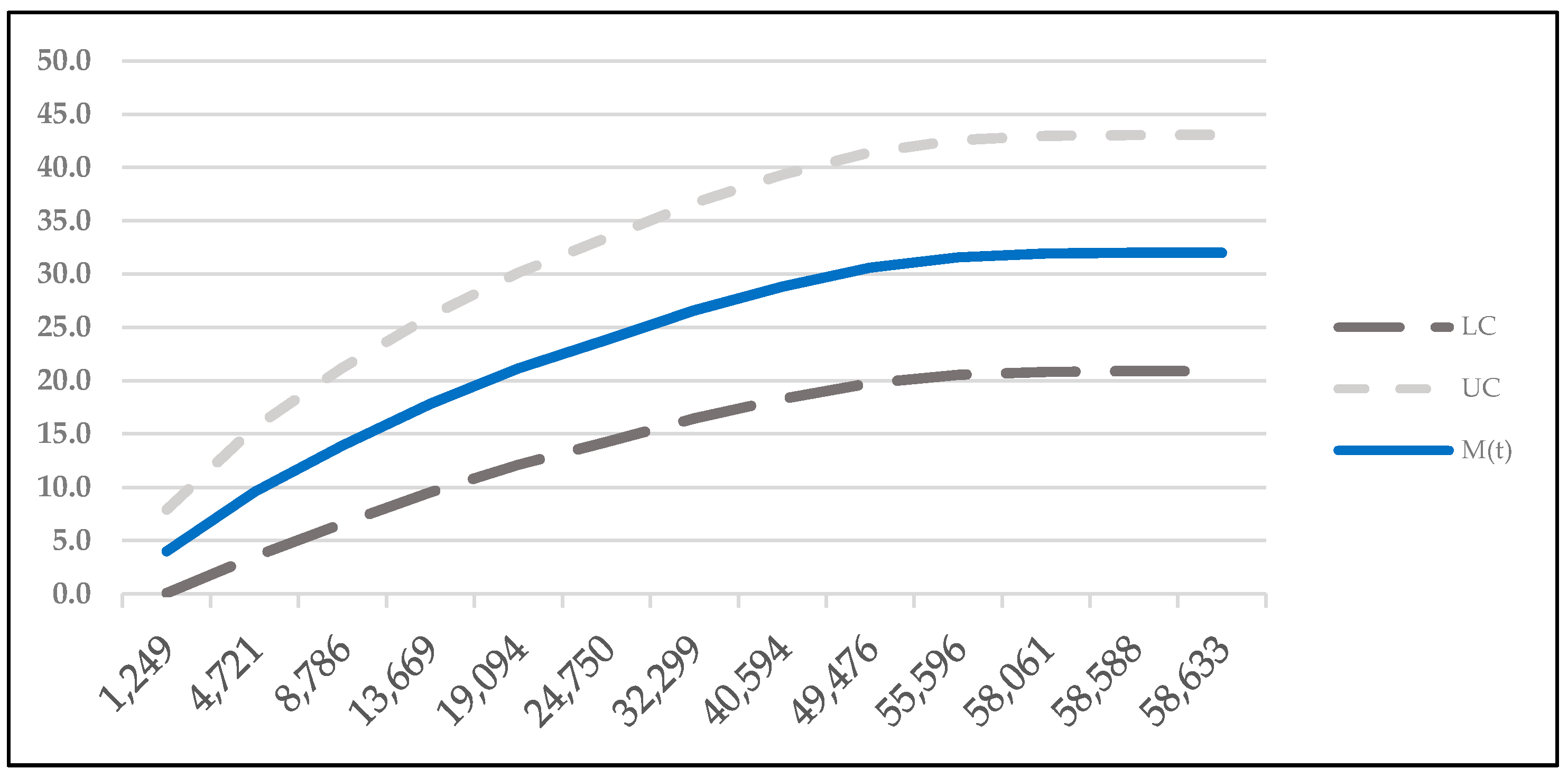
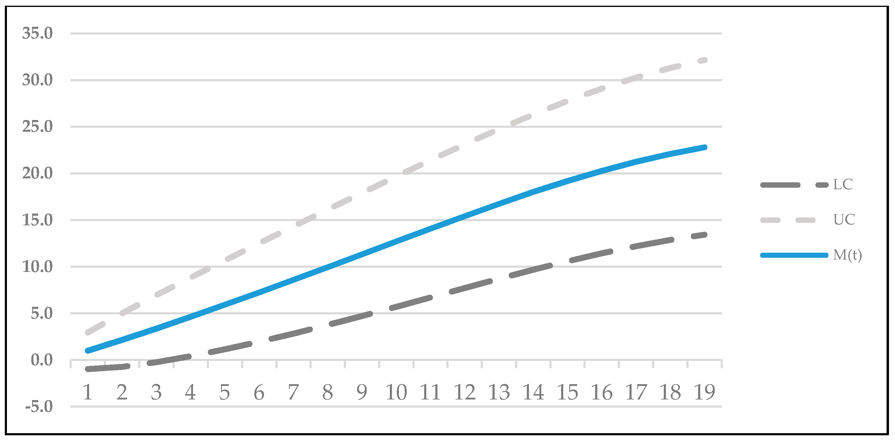
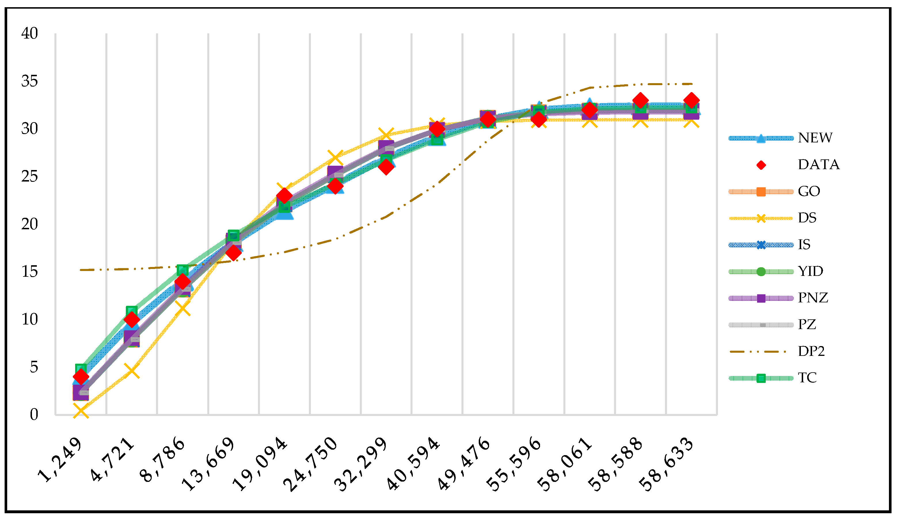
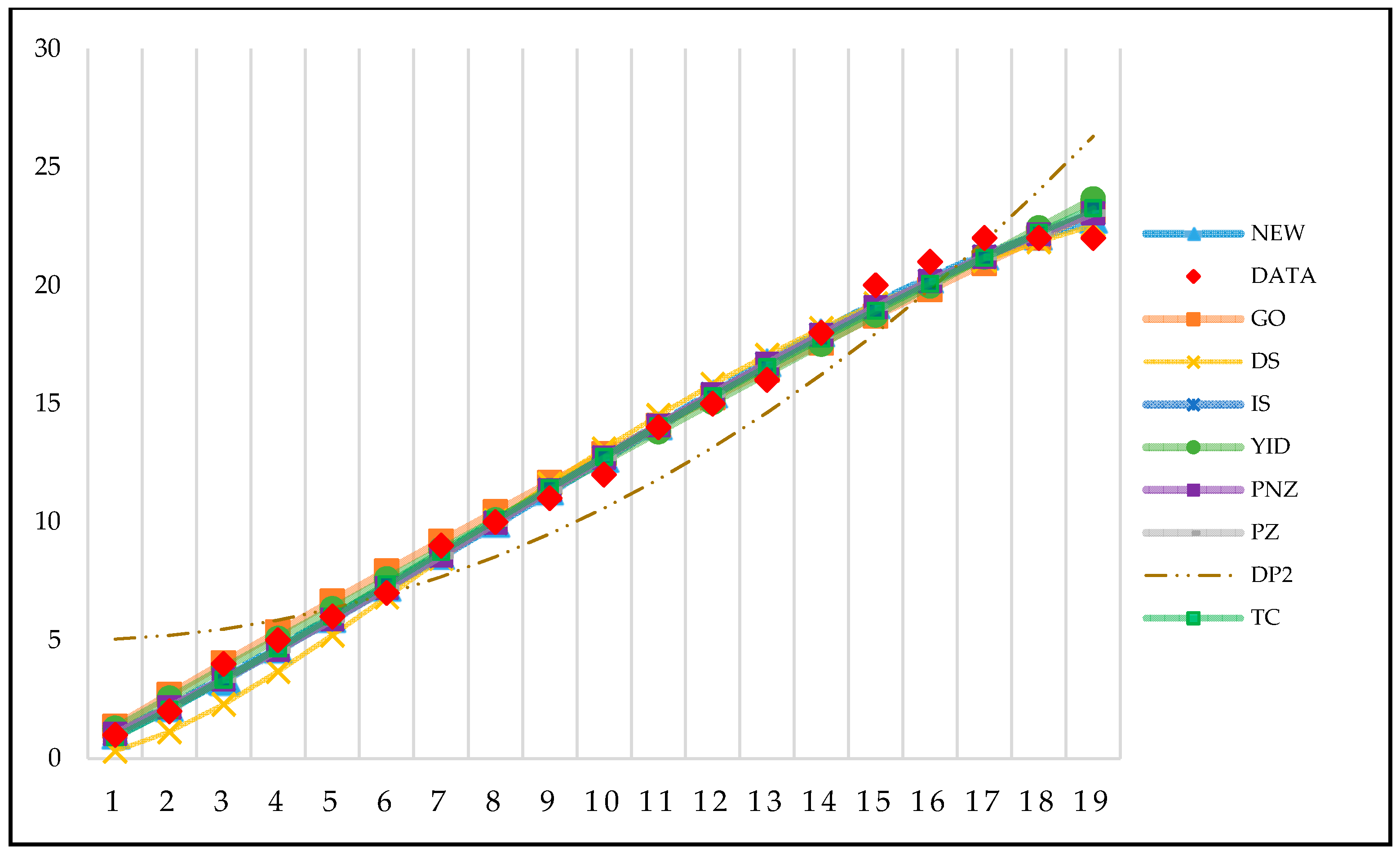
where ${\mathrm{z}}_{\mathsf{\alpha }/2}$ is the 100(1 − $\mathsf{\alpha }$) percentile of the standard normal distribution. Figure 2 and Figure 3 show the confidence interval of the proposed model for both data sets. Figure 4 and Figure 5 show the mean value functions of all the SRGMs for both data sets.

5. Software Release Policy

5.1. Optimal Release Time and Cost

In this section, we address the optimal release policy from the point of the view of time and cost. It can be helpful to find the optimal software release time $\left({\mathrm{T}}^{*}\right)$ that has the minimum expected total software development cost. Although the optimal release policy has been studied for decades, it is still a sensitive problem. For example, if the testing period is long, the software can be reliable, but the software development cost is increased. On the contrary, if the testing period is short, the product can be unreliable. Moreover, risk costs, such as the follow-up service cost, can be increased. Thus, it is crucial to find a balanced time point between release time and minimum cost.

Figure 6 shows the system development lifecycle considered in the following cost model, which includes the testing phase before release time T, the testing environment period, the warranty period, and the operational life in the actual field environment (that is usually quite different from the testing environment) [33].

The expected total software development cost $\mathrm{C}\left(\mathrm{T}\right)$ depends on various factors and it can be expressed as:

$$\mathrm{C}\left(\mathrm{T}\right)={\mathrm{C}}_0+{\mathrm{C}}_1\mathrm{T}+{\mathrm{C}}_2\mathrm{m}\left(\mathrm{T}\right){\mathsf{\mu }}_{\mathrm{Y}}+{\mathrm{C}}_3\left(1-\mathrm{R}\left(\mathrm{x}|\mathrm{T}\right)\right)+{\mathrm{C}}_4\left[\mathrm{m}\left(\mathrm{T}+{\mathrm{T}}_{\mathrm{W}}\right)-\mathrm{m}\left(\mathrm{T}\right)\right]{\mathsf{\mu }}_{\mathrm{W}},$$

(21)

where ${\mathrm{C}}_0$ is the set-up cost for the test, ${\mathrm{C}}_1\mathrm{T}$ is the cost of test, ${\mathrm{C}}_2\mathrm{m}\left(\mathrm{T}\right){\mathsf{\mu }}_{\mathrm{y}}$ is the expected cost to remove all failures detected by time T during the testing period, ${\mathrm{C}}_3\left(1-\mathrm{R}\left(\mathrm{x}|\mathrm{T}\right)\right)$ is the penalty cost of removing failures that occur after the system release time T, and ${\mathrm{C}}_4\left[\mathrm{m}\left(\mathrm{T}+{\mathrm{T}}_{\mathrm{W}}\right)-\mathrm{m}\left(\mathrm{T}\right)\right]{\mathsf{\mu }}_{\mathrm{W}}$ is the expected cost to remove all of the failures that are detected during the warranty period $\left[\mathrm{T},\mathrm{T}+{\mathrm{T}}_{\mathrm{W}}\right]$. Furthermore, it requires the assumption that the cost required to remove errors during the operating period is higher than that during the testing period and the time that is needed is much longer.

Finally, the expected total software cost can be calculated using the $\mathrm{m}\left(\mathrm{t}\right)$ function consisting of the estimated parameters. The primary purpose of the equation is to find the optimal software release time $\left({\mathrm{T}}^{*}\right)$ minimizing the expected total cost.

5.2. Results of Optimal Release Time and Cost

We apply the mean value function $\mathrm{m}\left(\mathrm{t}\right)$ obtained in Section 4 to the defined cost model $\mathrm{C}\left(\mathrm{T}\right)$ and consider coefficients in the cost model for the baseline case. The coefficients of the baseline case are listed in

Table 8. Baseline case.

C0	C1	C2	C3	C4	x	μx	μw	Tw
500	10	50	5000	500	10	0.1	0.1	10

.

Table 9. Optimal release time ${\mathrm{T}}^{*}$ and total cost $\mathrm{C}\left(\mathrm{T}\right)$ for ${\mathrm{T}}_{\mathrm{w}}$ (Case 1).

	Tw = 5		Tw = 10		Tw = 15		Tw = 20
	T*	C(T)	T*	C(T)	T*	C(T)	T*	C(T)
New	46.6	1166.8328	47	1172.8471	47.2	1176.2287	47.4	1178.2435

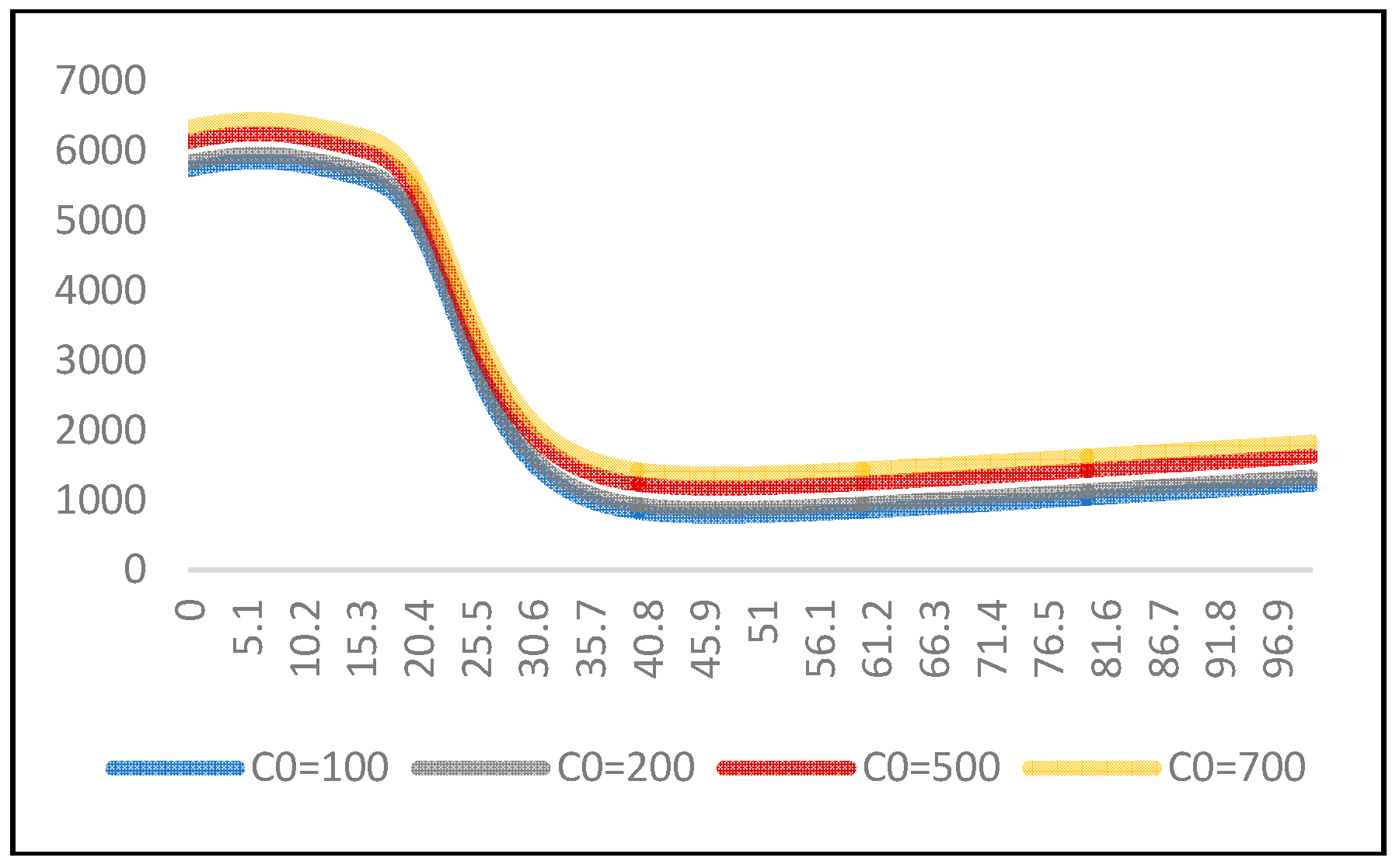
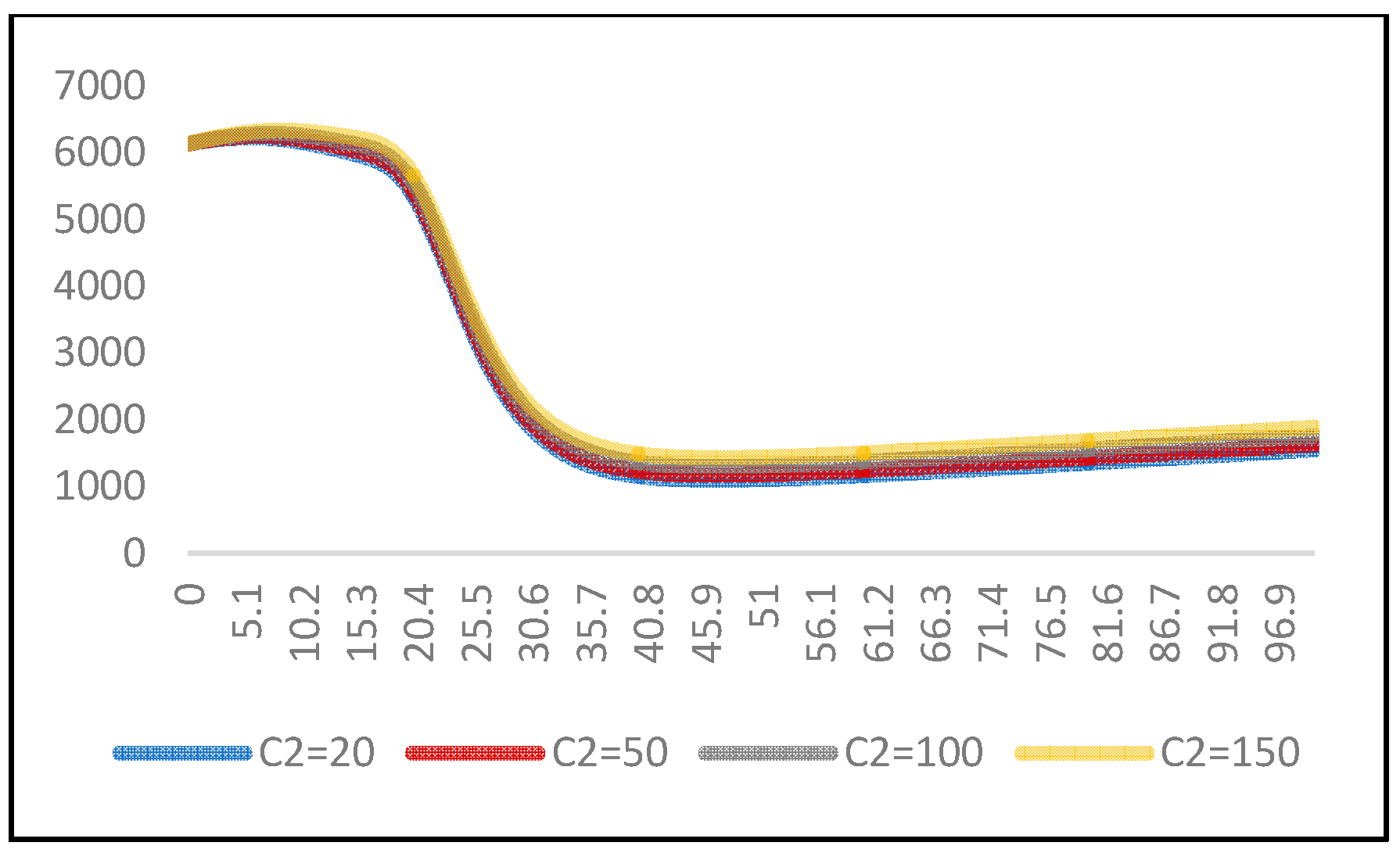
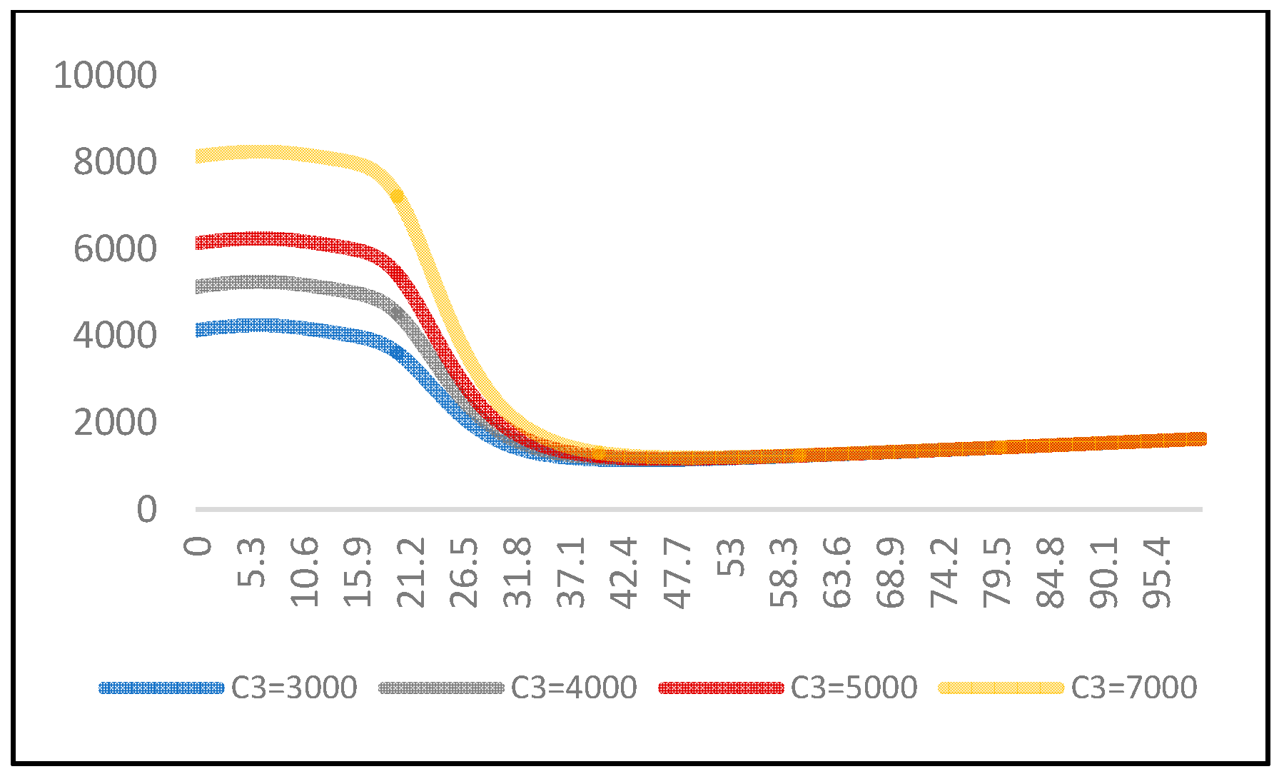
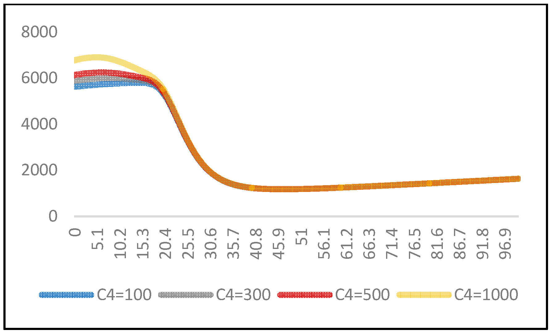
presents the values of release time and expected total cost under certain conditions derived from variation of the cost coefficients and warranty period ${\mathrm{T}}_{\mathrm{w}}$. Similarly, in

Table 10. Optimal release time ${\mathrm{T}}^{*}$ and total cost $\mathrm{C}\left(\mathrm{T}\right)$ for ${\mathrm{C}}_0$ (Case 2).

C0	Tw = 5		Tw = 10		Tw = 15		Tw = 20
	T*	C(T)	T*	C(T)	T*	C(T)	T*	C(T)
100	46.6	766.8328	47	772.8471	47.2	776.2287	47.4	778.2435
200	46.6	866.8328	47	872.8471	47.2	876.2287	47.4	878.2435
500	46.6	1166.8328	47	1172.8471	47.2	1176.2287	47.4	1178.2435
700	46.6	1366.8328	47	1372.8471	47.2	1376.2287	47.4	1378.2435

,

Table 11. Optimal release time ${\mathrm{T}}^{*}$ and total cost $\mathrm{C}\left(\mathrm{T}\right)$ for ${\mathrm{C}}_2$ (Case 3).

C2	Tw = 5		Tw = 10		Tw = 15		Tw = 20
	T*	C(T)	T*	C(T)	T*	C(T)	T*	C(T)
20	46.6	1089.6537	47	1095.6652	47.2	1099.0456	47.4	1101.0591
50	46.6	1166.8328	47	1172.8471	47.2	1176.2287	47.4	1178.2435
100	46.6	1295.4647	47	1301.4835	47.2	1304.8673	47.3	1306.8837
150	46.6	1424.0966	47	1430.1199	47.2	1433.5059	47.3	1435.5233

,

Table 12. Optimal release time ${\mathrm{T}}^{*}$ and total cost $\mathrm{C}\left(\mathrm{T}\right)$ for ${\mathrm{C}}_3$ (Case 4).

C3	Tw = 5		Tw = 10		Tw = 15		Tw = 20
	T*	C(T)	T*	C(T)	T*	C(T)	T*	C(T)
3000	43.4	1131.1875	43.8	1136.4696	44	1139.3614	44.1	1141.0439
4000	45.2	1150.9796	45.6	1156.6584	45.8	1159.8148	45.9	1161.6762
5000	46.6	1166.8328	47	1172.8471	47.2	1176.2287	47.4	1178.2435
7000	48.7	1191.5935	49.2	1198.1598	49.5	1201.9114	49.6	1204.1773

and

Table 13. Optimal release time ${\mathrm{T}}^{*}$ and total cost $\mathrm{C}\left(\mathrm{T}\right)$ for ${\mathrm{C}}_4$ (Case 5).

C4	Tw = 5		Tw = 10		Tw = 15		Tw = 20
	T*	C(T)	T*	C(T)	T*	C(T)	T*	C(T)
100	46.5	1166.5033	47	1172.3822	47.2	1175.6963	47.3	1177.6743
300	46.6	1166.6685	47	1172.6146	47.2	1175.9625	47.3	1177.9591
500	46.6	1166.8328	47	1172.8471	47.2	1176.2287	47.4	1178.2435
1000	46.6	1167.2435	47.1	1173.4273	47.3	1176.8886	47.4	1178.9461

appear the values for change of parameters of the $\mathrm{C}\left(\mathrm{T}\right)$ function. Figure 7, Figure 8, Figure 9, Figure 10 and Figure 11 illustrate Table 9, Table 10, Table 11, Table 12 and Table 13 when ${\mathrm{T}}_{\mathrm{w}}$ is 10. In addition, the baseline case is drawn as a red line.

In Table 9, ${\mathrm{T}}^{*}$ and $\mathrm{C}\left(\mathrm{T}\right)$ increase when the warranty period ${\mathrm{T}}_{\mathrm{w}}$ increases. Further, $\mathrm{C}\left(\mathrm{T}\right)$ increases when ${\mathrm{C}}_0$ increases in Table 10. In Table 11, Table 12 and Table 13, ${\mathrm{T}}^{*}$ and $\mathrm{C}\left(\mathrm{T}\right)$ increase when ${\mathrm{C}}_1$, ${\mathrm{C}}_3$, and ${\mathrm{C}}_4$ increase. As a result, ${\mathrm{C}}_0$ does not affect ${\mathrm{T}}^{*}$, but it affects $\mathrm{C}\left(\mathrm{T}\right)$. ${\mathrm{C}}_1$ affects ${\mathrm{T}}^{*}$, and has some effect on $\mathrm{C}\left(\mathrm{T}\right)$. ${\mathrm{C}}_3$ and ${\mathrm{C}}_4$ have a significant effect on ${\mathrm{T}}^{*}$ and $\mathrm{C}\left(\mathrm{T}\right)$.

6. Sensitivity Analysis

6.1. Sensitivity Analysis of Parameters

We conduct a sensitivity analysis of the parameters for the optimal release [38]. ${\mathrm{S}}_{\mathrm{T}}$ is defined as the relative change of release time when $\mathsf{\theta }$ is changed by 100p%, where $\mathsf{\theta }$ is a parameter of the mean value function, $\mathrm{m}\left(\mathrm{t}\right)$. ${\mathrm{S}}_{\mathrm{T}}$ can be expressed as:

$${\mathrm{S}}_{\mathrm{T}}=\frac{\mathrm{T}\left(\left(1+\mathsf{\theta }\right)\mathrm{P}\right)-\mathrm{T}\left(\mathrm{P}\right)}{\mathrm{T}\left(\mathrm{P}\right)}.$$

(22)

6.2. Results of Sensitivity Analysis

Table 14. Sensitivity analysis for parameters of the optimal release time.

	−30%	−20%	−10%	0	10%	20%	30%
a	0.022837	0.014165	0.006637	0	−0.005927	−0.011273	−0.016140
b	1.739638	0.498721	0.187518	0	−0.118787	−0.197279	−0.251138
$\mathsf{\alpha }$	−0.021859	−0.013792	−0.006561	0	0.006012	0.011565	0.016728
$\mathsf{\beta }$	−0.021811	−0.013763	−0.006547	0	0.006000	0.011543	0.016696
${\mathrm{T}}_0$	−0.000003	−0.000002	−0.000001	0	0.000001	0.000002	0.000003
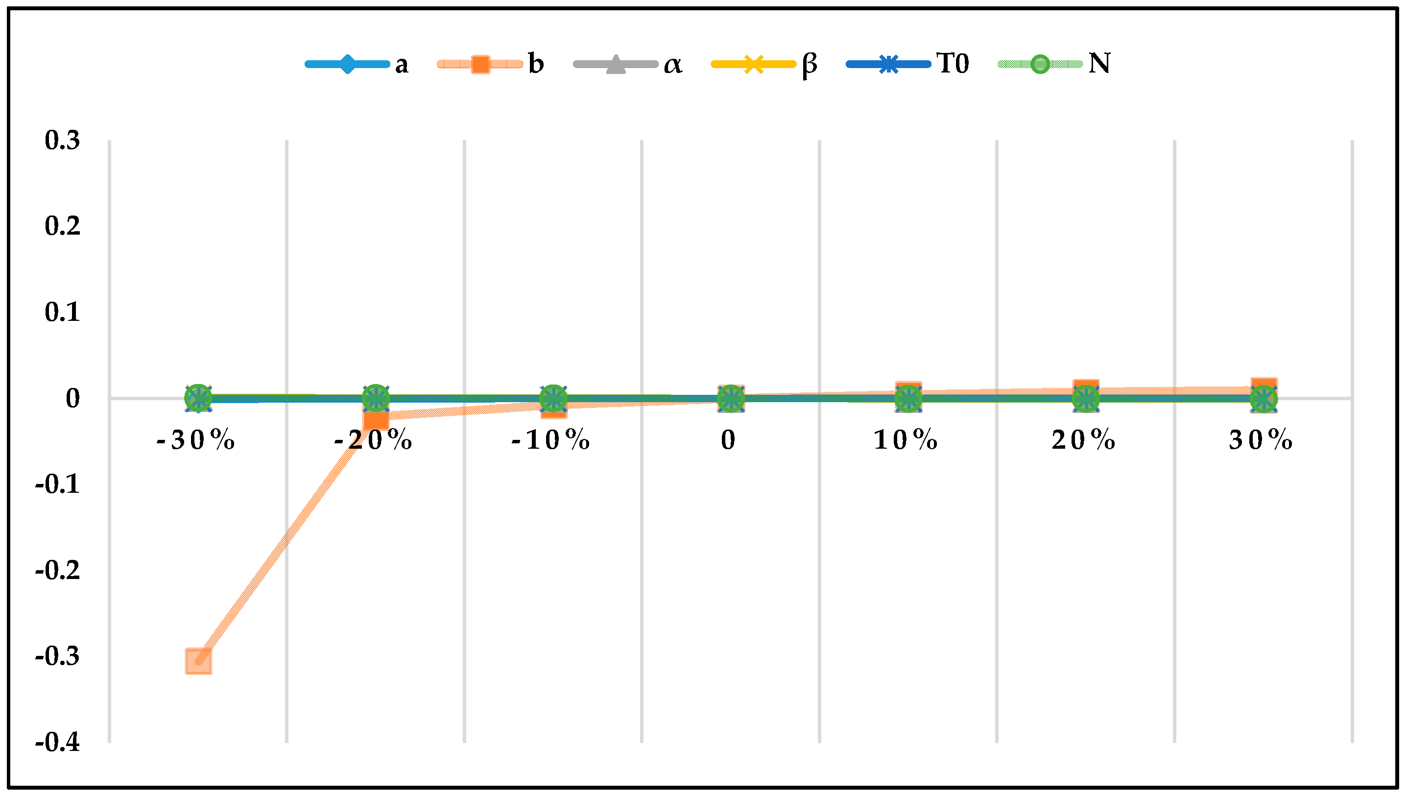
$\mathrm{N}$	−0.054793	−0.035748	−0.017538	0	0.016989	0.033519	0.049658

and Figure 12 reveal how much each parameter is changed for release time T. From Table 14, b is the most sensitive parameter and ${\mathrm{T}}_0$ is the most insensitive parameter. Moreover, the values in the sensitivity analysis of parameters $\mathsf{\alpha }$ and $\mathsf{\beta }$ are almost equal because the software reliability function has the same amount of variation when parameters $\mathsf{\alpha }$ and $\mathsf{\beta }$ vary. In brief, the optimal release time (${\mathrm{T}}^{*}$) increases with the decrease in $\mathrm{a}$ and $\mathrm{b}$. Furthermore, ${\mathrm{T}}^{*}$ decreases with the increase in $\mathsf{\alpha }$, $\mathsf{\beta }$, ${\mathrm{T}}_0$, and $\mathrm{N}$.

If the software is released too early, more resources will be required, such as risk cost, update cost, and human resources from the users and the development company. On the contrary, if the software is released too late, it will be necessary to assume higher cost of development. Therefore, the overestimation of $\mathsf{\alpha }$, $\mathsf{\beta }$, ${\mathrm{T}}_0$, and $\mathrm{N}$ and the underestimation of $\mathrm{a}$ and $\mathrm{b}$, which can lead to misestimations, such as underestimation of the optimal release time (${\mathrm{T}}^{*}$), should be avoided.

7. Conclusions

We suggested a new SRGM considering the start of actual debugging time for software affected by syntax errors. To compare it with several existing NHPP SRGMs, we applied two real data sets. Parameters for all models were estimated by the LSE method. In addition, common criteria were used to compare the goodness of fit in order to discuss the optimal model (Table 5 and Table 6). The values of the criteria of the proposed model are better than those of the other SRGMs, as listed in Table 1. The values of AIC for both data sets were not the lowest compared to those of the other models, but the proposed model, from the point of view of the other criteria, was the most significant. Then, we applied a cost model to the new proposed SRGM, and found out how much each parameter is changed regarding coefficients, release time, and cost.

In summary, the proposed model fits better than all the other models for both data sets. Through in Section 5, we found out variance of ${\mathrm{C}}_3$ and ${\mathrm{C}}_4$ affecting the field environment are greater than other coefficients. In order to establish the optimal release policy, it is necessary to subdivide the coefficients related to the field environment. As discussed in Section 6, $\mathrm{b}$ is the most sensitive parameter and ${\mathrm{T}}_0$ is the most insensitive parameter (in Table 14). Overestimation of $\mathsf{\alpha }$, $\mathsf{\beta }$, ${\mathrm{T}}_0$, and $\mathrm{N}$ and underestimation of $\mathrm{a}$ and $\mathrm{b}$ have to be avoided because they can lead to misestimation of the optimal release time.

Recently, many researchers have studied software reliability model considering software development environment. Likewise, we studied software reliability model considering uncertainty of software development environment like syntax error. Then, we provided optimal release policies having minimized the total development cost for various environments. Therefore, when the other data sets and various environments are given, the proposed model is beneficial.

8. Future Research

A further direction of this study will be to find diverse and more recent data sets to prove clearly the goodness of fit of the new model. In addition, we estimated parameters using LSE method. Therefore, we need to apply MLE or Bayesian inference to estimate parameters, and also need to consider the change-point.

References

1. Clarke, P.; O’Connor, R.V. The situational factors that affect the software development process: Towards a comprehensive reference framework. Inf. Softw. Technol. 2012, 54, 433–447. [Google Scholar] [CrossRef] [Green Version]
2. Musa, J.D.; Iannino, A.; Okumoto, K. Software Reliability: Measurement, Prediction, and Application; McGraw-Hill: New York, NY, USA, 1987. [Google Scholar]
3. Yamada, S.; Ohba, M.; Osaki, S. S-shaped reliability growth modeling for software fault detection. IEEE Trans. Reliab. 1983, 32, 475–484. [Google Scholar] [CrossRef]
4. Yamada, S.; Ohba, M.; Osaki, S. Software Reliability Growth Models with Testing-effort. IEEE Trans. Reliab. 1986, 35, 19–23. [Google Scholar] [CrossRef]
5. Quadri, S.M.K.; Ahmad, N.; Peer, M.A. Software optimal release policy and reliability growth modeling. In Proceedings of the 2nd National Conference on Computing for Nation Development, New Delhi, India, 8–9 February 2008; pp. 423–431. [Google Scholar]
6. Ahmd, N.; Khan, M.G.M.; Rafi, L.S. A study of testing-effort dependent inflection S-shaped software reliability growth models with imperfect debugging. Int. J. Qual. Reliab. Manag. 2009, 27, 89–110. [Google Scholar] [CrossRef]
7. Pham, H.; Zhang, X. An NHPP software reliability models and its comparison. Int. J. Reliab. Qual. Saf. Eng. 1997, 4, 269–282. [Google Scholar] [CrossRef]
8. Pham, H.; Zhang, X. Software Reliability and Cost Models with Testing Coverage. Eur. J. Oper. Res. 2003, 145, 443–454. [Google Scholar] [CrossRef]
9. Teng, X.; Pham, H. A new methodology for predicting software reliability in the random field environments. IEEE Trans. Reliab. 2006, 55, 458–468. [Google Scholar] [CrossRef]
10. Pham, H. Loglog Fault-Detection Rate and Testing Coverage Software Reliability Models Subject to Random Environments. Vietnam J. Comput. Sci. 2014, 1, 39–45. [Google Scholar] [CrossRef]
11. Inoue, S.; Ikeda, J.; Yamda, S. Bivariate change-point modeling for software reliability assessment with uncertainty of testing-environment factor. Ann. Oper. Res. 2016, 244, 209–220. [Google Scholar] [CrossRef]
12. Li, Q.; Pham, H. A testing-coverage software reliability model considering fault removal efficiency and error generation. PLoS ONE 2017, 12, e0181524. [Google Scholar] [CrossRef] [PubMed]
13. Song, K.Y.; Chang, I.H.; Pham, H. A three-parameter fault-detection software reliability model with the uncertainty of operating environments. J. Syst. Sci. Syst. Eng. 2017, 26, 121–132. [Google Scholar] [CrossRef]
14. Song, K.Y.; Chang, I.H.; Pham, H. A Software Reliability Model with a Weibull Fault Detection Rate Function Subject to Operating Environments. Appl. Sci. 2017, 7, 983. [Google Scholar] [CrossRef]
15. Song, K.Y.; Chang, I.H.; Pham, H. An NHPP Software Reliability Model with S-Shaped Growth Curve Subject to Random Operating Environments and Optimal Release Time. Appl. Sci. 2017, 7, 1304. [Google Scholar] [CrossRef]
16. Zhu, M.; Pham, H. A two-phase software reliability modeling involving with software fault dependency and imperfect fault removal. Comput. Lang. Syst. Struct. 2018, 53, 27–42. [Google Scholar] [CrossRef]
17. Zhu, M.; Pham, H. A software reliability model incorporating martingale process with gamma-distributed environmental factors. Ann. Oper. Res. 2018, 1–22. [Google Scholar] [CrossRef]
18. Zeephongsekul, P.; Jayasinghe, C.L.; Fiondella, L.; Nagaraju, V. Maximum-Likelihood Estimation of Parameters of NHPP Software Reliability Models Using Expectation Conditional Maximization Algorithm. IEEE Trans. Reliab. 2016, 65, 1571–1583. [Google Scholar] [CrossRef]
19. Candini, F.; Gioletta, A. A Bayesian Monte Carlo-based algorithm for the estimation of small failure probabilities of systems affected by uncertainties. Reliab. Eng. Syst. Saf. 2016, 153, 15–27. [Google Scholar] [CrossRef]
20. Caiuta, R.; Pozo, A.; Vergilio, S.R. Meta-learning based selection of software reliability models. Automat. Softw. 2017, 24, 575–602. [Google Scholar] [CrossRef]
21. Tamura, Y.; Yamda, S. Software Reliability Model Selection Based on Deep Learning with Application to the Optimal Release Problem. J. Ind. Eng. Manag. Sci. 2018, 2016, 43–58. [Google Scholar] [CrossRef]
22. Tamura, Y.; Matsumoto, S.; Yamada, S. Software Reliability Model Selection Based on Deep Learning. In Proceedings of the International Conference on Industrial Engineering Management Science and Application, Jeju, Korea, 23–26 May 2016; pp. 1–5. [Google Scholar]
23. Wang, J.; Zhang, C. Software reliability prediction using a deep learning model based on the RNN encoder-decoder. Reliab. Eng. Syst. Saf. 2018, 170, 73–82. [Google Scholar] [CrossRef]
24. Kim, K.C.; Kim, Y.H.; Shin, J.H.; Han, K.J. A Case Study on Application for Software Reliability Model to Improve Reliability of the Weapon System. J. KIISE 2011, 38, 405–418. [Google Scholar]
25. Goel, A.L.; Okumoto, K. Time dependent error detection rate model for software reliability and other performance measures. IEEE Trans. Reliab. 1979, 28, 206–211. [Google Scholar] [CrossRef]
26. Ohba, M. Inflexion S-shaped software reliability growth models. In Stochastic Models in Reliability Theory; Osaki, S., Hatoyama, Y., Eds.; Springer: Berlin, Germany, 1984; pp. 144–162. [Google Scholar]
27. Yamada, S.; Tokuno, K.; Osaki, S. Imperfect debugging models with fault introduction rate for software reliability assessment. Int. J. Syst. Sci. 1992, 23, 2241–2252. [Google Scholar] [CrossRef]
28. Pham, H.; Nordmann, L.; Zhang, X. A general imperfect software debugging model with S-shaped fault detection rate. IEEE Trans. Reliab. 1999, 48, 169–175. [Google Scholar] [CrossRef]
29. Pham, H. Software Reliability Models with Time Dependent Hazard Function Based on Bayesian Approach. Int. J. Autom. Comput. 2007, 4, 325–328. [Google Scholar] [CrossRef]
30. Chang, I.H.; Pham, H.; Lee, S.W.; Song, K.Y. A testing-coverage software reliability model with the uncertainty of operation environments. Int. J. Syst. Sci. Oper. Logist. 2014, 1, 220–227. [Google Scholar]
31. Pham, H. System Software Reliability; Springer: London, UK, 2006; p. 13. [Google Scholar]
32. Li, Q.; Pham, H. NHPP software reliability model considering the uncertainty of operating environments with imperfect debugging and testing coverage. Appl. Math. Model. 2017, 51, 68–85. [Google Scholar] [CrossRef]
33. Akaike, H. A new look at statistical model identification. IEEE Trans. Autom. Control 1974, 19, 716–719. [Google Scholar] [CrossRef]
34. Pillai, K.; Nair, V.S. A model for software development effort and cost estimation. IEEE Trans. Softw. Eng. 1997, 23, 485–497. [Google Scholar] [CrossRef]
35. Xu, J.; Yao, S. Software Reliability Growth model with Partial Differential Equation for Various Debugging Processes. Math. Probl. Eng. 2016, 2016, 1–13. [Google Scholar] [CrossRef]
36. Anjum, M.; Haque, M.A.; Ahmad, N. Analysis and ranking of software reliability models based on weighted criteria value. J. Inform. Technol. Comput. Sci. 2013, 2, 1–14. [Google Scholar] [CrossRef]
37. Daniel, R.J.; Zhang, X. Some successful approaches to software reliability modeling in industry. J. Syst. Softw. 2005, 74, 85–99. [Google Scholar]
38. Li, X.; Xie, M.; Ng, S.H. Sensitivity analysis of release time of software reliability models incorporating testing effort with multiple change-points. Appl. Math. Model. 2010, 34, 3560–3570. [Google Scholar] [CrossRef]
Figure 1. Testing time infrastructure.
Applsci 08 01483 g001
Figure 2. Confidence interval of the new proposed model for data set 1.
Applsci 08 01483 g002
Figure 3. Confidence interval of the new proposed model for data set 2.
Applsci 08 01483 g003
Figure 4. m(t) of all SRGMs for data set 1.
Applsci 08 01483 g004
Figure 5. m(t) of all SRGMs for data set 2.
Applsci 08 01483 g005
Figure 6. System development lifecycle.
Applsci 08 01483 g006
Figure 7. T * and C ( T ) for T w   (Table 9).
Applsci 08 01483 g007
Figure 8. T * and C ( T ) for T w = 10 (Table 10).
Applsci 08 01483 g008
Figure 9. T * and C ( T ) for T w = 10 (Table 11).
Applsci 08 01483 g009
Figure 10. T * and C ( T ) for T w = 10 (Table 12).
Applsci 08 01483 g010
Figure 11. T * and C ( T ) for T w = 10 (Table 13).
Applsci 08 01483 g011
Figure 12. Sensitivity analysis for parameters of the optimal release time.
Applsci 08 01483 g012