Abstract
Longitudinal-connected air suspension has been proven to have desirable dynamic load-sharing performances for multi-axle heavy vehicles. However, optimization approaches towards the improvement of comprehensive vehicle performance through the geometric design of longitudinal-connected air suspension have been considerably lacking. To address this, based on a 5-degrees-of-freedom nonlinear model of a three-axle semi-trailer with longitudinal air suspension, taking the changes of driving conditions (road roughness, speed, and load) into account, a height control strategy of the longitudinal-connected air suspension was proposed. Then, in view of the height of the air spring under various driving conditions, the support vector regression method was employed to fit the relationship models between the performance indices and the driving conditions, as well as the suspension geometric parameters (inside diameters of the air line and the connectors). Finally, to tackle the uncertainties of driving conditions in the optimization of suspension geometric parameters, a double-loop multi-objective particle swarm optimization algorithm (DL-MOPSO) was put forward based on the interval uncertainty theory. The simulation results indicate that compared with the longitudinal-connected air suspension using two traditional geometric parameters, the optimization ratios for dynamic load sharing coefficient and root-mean-square acceleration at various spring heights are between −1.04% and 20.75%, and 1.44% and 35.1%, respectively. Therefore, based on the signals measured from the suspension height sensors, through integrated control of inflation/deflation valves of air suspensions, as well as the valves’ inside connectors and air lines, the proposed DL-MOPSO algorithm can improve the comprehensive driving performance of the longitudinal-connected three-axle semi-trailer effectively, and in response to changes in driving conditions.
1. Introduction
The suspension system of multi-axle trucks is an important component that affects the driving performance of vehicles. In previous studies, the optimization and control of truck suspensions mainly targeted road-friendliness, ride comfort, and steering stability [1,2,3], but not enough attention has been paid to an important performance index that affects the safety of the road traffic, namely, the dynamic load-sharing performance of the multi-axle groups. The dynamic load-sharing performance of the multi-axle groups refers to the ability to distribute the load evenly between the axles within the multi-axle groups during driving [4]. Favorable dynamic load-sharing can reduce the peak forces from tires: on the one hand, it can prevent tire blowout caused by single-axle overloading and the braking failure caused by load transfer during braking; on the other hand, it is closely related to the road-friendliness, able to delay the occurrence of ruts, cracks, looseness, pits, and peeling on roads [5]. Therefore, the dynamic load-sharing of multi-axle trucks is a comprehensive index covering driving safety and road-friendliness.
Load-sharing is relatively weak for leaf springs (usually employing centrally pivoted walking beams, trunnion shafts, etc.) and unconnected air suspensions of multi-axle trucks [6,7]. To address this issue, an Australian design for longitudinal-connected air suspensions connects the air springs in the axle groups on the same side through larger-than-industry air lines and connectors so that air could be exchanged between air bags more readily. This kind of suspension not only has a damping effect similar to that of air suspension with additional air chambers, but also, when applied to the multi-axle groups of tractors or semi-/full-trailers, can have the air bag force transferred rapidly between different axles through the air lines and connectors, thus effectively improving the load-sharing of vehicles [8].
Many on-road tests have been performed to analyze the performance of the longitudinal-connected air suspension. The Organization for Economic Co-operation and Development (OECD) indicated that the load-sharing coefficient (an indicator for load-sharing capacity) of multi-axle trucks in western countries ranged from 0.904 to 0.925 [9]. Studies commissioned by the National Road Transport Commission of Australia found that installation of larger air lines on multi-axle air suspension increased longitudinal air flow between air springs on adjacent axles [10]. The Queensland Department of Main Roads discovered that improvements in dynamic load-sharing coefficient (DLSC) of 4–30% for a tri-axle coach and 37–77% for a tri-axle semi-trailer were obtained by altering the conventional-sized longitudinal air connection (three 6.5 mm inside diameter connectors connecting 6.5 mm inside diameter air lines) to a larger air connection (three 20 mm inside diameter connectors at the air springs connecting 50 mm inside diameter air lines) [8]. However, due to the limitations of on-road tests, only vehicle speed and a limited number of air connections were considered in most tests, such that the effect of some other factors, e.g., the static absolute air pressure of the air spring, static height of the air spring, and load-sharing, were not able to be taken into account.
Limitations of on-road tests can be addressed by developing realistic models of connected air suspension. Xu et al. developed a 4-degrees-of-freedom (DOF) half-vehicle model and compared the transferring characteristics between the laterally interconnected and non-interconnected air suspension. It was found that the laterally interconnected air suspension could significantly decrease the amplitude of roll angle [11]. Li et al. developed an 8-DOF mathematical model of a car with laterally interconnected air suspension [12,13]. It is indicated that these suspensions outperformed unconnected suspensions in terms of vibration isolation and torsion elimination. With respect to the modelling of longitudinal-connected air suspension, Davis proposed a model of a tri-axle semi-trailer with longitudinal-connected air suspensions [8], and used a variable “load-sharing fraction” to represent the load-sharing ability of the suspension. However, the physical meaning of the variable was not explored completely, leaving that detail for others to study. More advanced models of similar tri-axle semi-trailers have been developed by Roebuck and Kat based on aerodynamics and thermodynamics [14,15]. In these models, isothermal gas compression process was assumed; in addition, the effective areas of the air springs were simplified as constants while the vehicle was travelling. Regarding these issues, a more accurate nonlinear model of a tri-axle longitudinal-connected air suspension was formulated by Chen et al. [16,17]. Based on this model, the effects of driving conditions (road class, vehicle speed, and vehicle load) and air suspension parameters (static height and static absolute air pressure of air spring, inside diameters of air line and connector) on dynamic load-sharing were analyzed comprehensively. It is indicated that the air line diameter and the connector diameter are two key geometric factors affecting DLSC, and the influence of air line diameter on load-sharing is more significant than that of the connector. Zhu et al. derived the system equations of a pitch-plane 4-DOF half-car with longitudinal-connected air suspension. The effects of pipe length, pipe diameter, and the local loss ratio factor on the vehicle pitch transmissibility properties, rather than the load-sharing, were investigated [18].
In summary, achievements have been made in the analysis of the load-sharing of longitudinal-connected air suspension based on both theoretical modeling and field tests. Although it is widely recognized that air line diameter and connector diameter are important factors affecting load-sharing, the optimization of these geometric parameters towards integrated driving performances, such as load-sharing and ride comfort, has rarely been reported. For electronically controlled air suspension, under certain height of the air springs, road roughness, driving speed, and vehicle load are all uncertain variables (change within certain ranges) and have a nonlinear relationship with the load-sharing. Therefore, the determination of the key geometric parameters of longitudinal-connected air suspension is a problem for uncertain, nonlinear, and multi-objective optimization.
The traditional stochastic programming method and fuzzy programming method can solve the uncertain optimization problems, but a large amount of uncertainty information is needed to construct the exact probability distribution or fuzzy membership function of the variable [19,20]. Since it is very difficult to get such uncertain information, these two methods are strongly limited in applications. By introducing order relations of interval numbers, Moore et al. proposed an interval number optimization method to transform the uncertainty optimization problem into a deterministic optimization problem of inner and outer nesting [21,22]. This method only needs to get the possible ranges of uncertain parameters rather than their exact distributions. Thus, it can reduce the difficulty of uncertainty optimization effectively and it has been widely employed for optimization in various engineering fields [23,24].
By introducing the interval number optimization method, the uncertain, nonlinear, and multi-objective optimization problem can be transformed into a nonlinear certain multi-objective optimization problem subject to two loops of nesting. One issue associated with the new problem after the transformation is that the objective functions are usually discontinuous and non-derivable; traditional gradient-based optimization methods, such as the steepest descent method and gradient projection method, have difficulties in solving such problems [25]. However, heuristic algorithms can overcome the difficulty in solving optimization problems caused by discontinuity and non-derivativity [26,27]. Another issue associated with the new problem is that owing to two loops of nesting, the repeated iterations of the inner and outer algorithms bring burdens to the computational process. Accordingly, high accuracy and efficiency are necessary for the optimization algorithm. Compared with other heuristic optimization algorithms, particle swarm optimization (PSO) features faster iteration speed, fewer parameters to be adjusted, simpler structure, and stronger capacity for global search [28,29].
Therefore, considering the uncertainty of the road roughness, driving speed, and vehicle load, this paper combines interval number optimization with multi-objective particle swarm optimization (MOPSO), and proposes a double-loop multi-objective particle swarm optimization (DL-MOPSO) algorithm to optimize the key geometric parameters of the longitudinal-connected air suspension, focusing on the comprehensive driving performance. In the DL-MOPSO algorithm, the inner loop algorithm is used to calculate the interval range of the target function when the uncertain variable is changing, while the outer loop algorithm is used for global optimization of the inner diameters of the optimal air lines and connectors.
The rest of the paper is organized as follows: Firstly, a nonlinear coupling model between road excitation and a tri-axle semi-trailer with longitudinal-connected air suspensions is described briefly. The strategy for controlling the height of the longitudinal-connected air suspension is designed, taking road roughness, driving speed, and vehicle load into account. Secondly, at each spring height, the relationships of the load-sharing and ride comfort indices with the changes of the driving conditions and suspension parameters are fitted, respectively, based on support vector regression. Finally, based on the interval uncertainty theory, a DL-MOPSO algorithm is designed to optimize the inner diameters of the air lines and connectors when the driving conditions are changing. Moreover, the effectiveness and robustness of the DL-MOPSO algorithm are analyzed by comparing the optimized results with the results using conventional-sized longitudinal-connected air suspension, under the circumstances of various spring heights and driving conditions.
2. Mathematic Models and Load-Sharing Criteria
2.1. Mathematic Models of the Tri-Axle Semi-Trailer and Road Roughness Excitation
A basic half-model representing a typical tri-axle semi-trailer with longitudinal-connected air suspension in most western countries was employed, as shown in Figure 1. This model includes 5-DOF, which are vertical displacement of sprung mass and three unsprung masses, z, x1, x2, x3, as well as the pitch angle of the sprung mass .
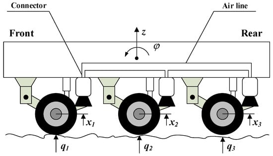
Figure 1.
Schematic of the tri-axle semi-trailer with longitudinal-connected air suspension.
The equations of motion of the semi-trailer are given by
where mt1, mt2, mt3 and q1, q2, q3 are the unsprung masses and road excitations of the three axles, respectively; m is the sprung mass of the semi-trailer; J is the moment of inertia of the gross sprung mass around the lateral axis; Ps1, Ps2, Ps3 and As1, As2, As3 are the dynamic absolute air pressures and dynamic effective areas of the three air springs, respectively; P0 is atmospheric pressure; l is the wheelbase; c1, c2, c3 are the damping coefficients of three dampers; and kt1, kt2, kt3 are the stiffness of the three tires.
In order to solve the above equations, a detailed model of longitudinal-connected tri-axle air suspension is needed to express Ps1, Ps2, and Ps3 as functions of the 5 variables (5 DOF). Specifically, an adiabatic process is assumed for the air inside air springs when the vehicle is travelling, and the air flow inside the connectors is considered to be an incompressible steady flow [15,30]. This model correlated well with the measurements. A concise spectral model is used in this study to represent the road roughness excitations. This vehicle–road integrated model takes the nonlinearity of the air transmission between the air springs into account, and thus correlates well with the experimental results of field tests. The details of the models and their experimental validation can be found in the previous work of the authors [16]. To avoid repetition, they are not described in this paper. Parameters of the longitudinal-connected tri-axle semi-trailer model are tabulated in Table 1.

Table 1.
Parameters of the longitudinal-connected tri-axle semi-trailer model (conventional-size longitudinal connection).
The prototype of the tri-axle semi-trailer with Kenworth Airglide 200 longitudinal-connected air suspension was tested on three typical urban road sections at speeds ranging from 60 km/h to 80 km/h [16]. Strain gauges (one per hub) were mounted on the neutral axis of each axle between the spring and the hub to record the shear force on the hubs, i.e., air spring force, and accelerometers were mounted as closely as possible to each hub and to the corresponding upper positions at the chassis to derive the height of each air spring. In addition, six air pressure transducers were employed to obtain the pressures inside the air springs.
Based on the experimental data, the effective area of each air spring was obtained by dividing the respective shear force by the respective pressure inside the air spring, and the volume of each air spring was derived by multiplying the respective effective area by the respective spring height. Thus, the dynamic effective area of each air spring is approximated as a function of the dynamic height of the corresponding air spring y, i.e.,
The effective area multiplied by the dynamic spring height yields
2.2. Load-Sharing Criteria
Criteria need to be chosen to evaluate the load-sharing of the semi-trailer. A metric often used to characterize the magnitude of dynamic forces of the ith wheel in an axle group is the DLC (dynamic load coefficient) [6], defined as
where denotes the standard deviation of Fi(j), which is the instantaneous force at wheel i (); and Fmean(i) denotes the mean wheel-force of wheel i. Although DLC is usually referred to as a road-friendliness criterion and has been criticized for not being mutually exclusive with another load-sharing criterion, the load-sharing coefficient (LSC), it still has been widely used as one measure to differentiate suspension types from each other (e.g., steel vs air) [3,4,31].
De Pont pointed out that LSC does not address dynamic load-sharing [32]. The DLSC was proposed as an alternative to LSC to account for the dynamic nature of wheel-forces and instantaneous load-sharing during travel, and is defined as [32]
The dynamic load-sharing of wheel i, DLSi(j), is
where n is the number of wheels on one side of an axle group, and k is the number of terms in the dataset.
In this study, the average DLSC of tires on the same side of the semi-trailer axle group was employed as a metric of load-sharing.
3. Control Strategy of Air Spring Height
The Kenworth Airglide 200 longitudinal-connected air suspensions investigated in this paper are passive suspensions. In order to enhance their comprehensive driving performance preliminarily, the air spring height control strategy shall first be designed based on the driving conditions. The natural frequency of the air suspension is expressed as
where f, , and m1 indicate the natural frequency of air suspension, spring stiffness, and sprung mass, respectively. is formulated as [33]
Ps10 changes with the sprung mass (Ps10 = m1g/As1 + p0); by introducing Equations (6) and (7) into Equation (12), the air spring stiffness at different heights can be obtained.
The design range for the natural frequency of rear suspension of the semi-trailers is 1.70~2.17 Hz [34]. Based on Equations (11) and (12), the proper ranges of spring heights can be derived with different sprung masses [35], and the optimal heights were determined as the medians of the ranges. Therefore, four control heights were set for the air suspension [33], specifically as follows:
I. In time of load-free idling and driving (when the actual load is less than 1/2 of the full load, it is defined as no load), the height of the spring is H0 (0.16 m).
II. In time of full load (when the actual load is equal to or more than 1/2 of the full load, it is defined as a full load), the spring height is set based on the vehicle speed and road condition as follows:
(1) In the case that the vehicle is kept static or moving at low speed (speed < 50 km/h), when the road is in good condition, the spring height is set to H1 (0.13 m); when the road condition is relatively poor, the spring height is set to H2 (0.15 m). The number of times that the height signal from the suspension height sensor exceeds the calibrated height value within an observation period (0.5 s) is recorded as N. If N is greater than 4, the road condition is considered as poor; otherwise, the road condition is good.
(2) If the vehicle is moving at high speed (speed > 70 km/h), when the road is in good condition, the spring height is set to H3 (0.11 m).
(3) 50~70 km/h is the hysteretic interval of the speed [33]. Hysteresis of 20 km/h is provided to prevent frequency occurrence of height level changes during travelling.
4. Development of Multi-Objective Optimization Functions for Comprehensive Driving Performance
The optimization of key geometric parameters of longitudinal-connected air suspension was respectively undertaken with each spring height. As indicated in Section 2.2, the average DLSC of tires on the same side of the semi-trailer axle group was selected as the index for evaluating load-sharing. The root mean square of the acceleration of the sprung mass (a) was selected as the ride comfort index.
4.1. Fitting Models of Evaluation Indices Based on Support Vector Regression
For a certain spring height, IRI (international roughness index), vehicle speed, and load vary within a certain range. Besides this, during the process of manufacturing, the inner diameter of the air pipe is no smaller than that of the connector. Table 2 shows the ranges of the variables at different spring heights.
Table 2.
Ranges of variables at different spring heights.
A full factorial experiment method was employed for the simulation of the vehicle–road coupling model described in Section 2.1. For each spring height, each uncertain variable was set to three levels, and each design variable was set to four levels [36]. Eliminating the experimental schemes in which the inner diameter of the air pipe is smaller than that of the connector, a total of 270 schemes remained. Simulation results of 220 schemes, which were randomly selected from the 270 schemes, were used for training of the fitting model, while the simulation results of the other 50 schemes were employed for the performance testing of the fitting model. Since support vector regression (SVR) features favorable fitting precision, fitting efficiency, and wide application range [37], it was used to fit the regression models of DLSC and a with the changes of the uncertain and design variables, respectively, based on the simulation results of the training schemes. The regression models are
where , are the expressions of DLSC and a after fitting via SVR, respectively; is the design vector; is the uncertain vector; l = 220; and are Lagrange multipliers, j = 1, 2; is the kernel function; is the support vector; ; and is the bias term.
Figure 2 shows the comparisons between the simulation values of Simulink models and the fitted values of SVR models using the test schemes. The coefficient of determination (R2) was chosen to test the goodness of fit of the SVR models. It is shown in the figure that the values of R2 are close to 1 for both the DLSC and a, which means that the accuracy of the SVR models is desirable. Thus, the SVR models can be used as the internal particle swarm fitness functions of the subsequent DL-MOPSO algorithm.
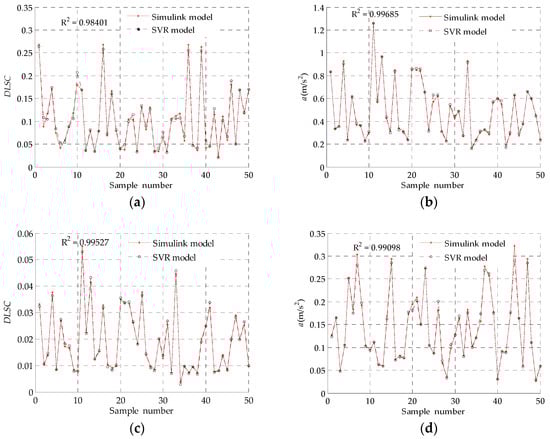
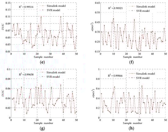
Figure 2.
(a) Comparisons of dynamic load-sharing coefficient (DLSC) between the two models at the spring height of H0; (b) Comparisons of a between the two models at the spring height of H0; (c) Comparisons of DLSC between the two models at the spring height of H1; (d) Comparisons of a between the two models at the spring height of H1; (e) Comparisons of DLSC between the two models at the spring height of H2; (f) Comparisons of a between the two models at the spring height of H2; (g) Comparisons of DLSC between the two models at the spring height of H3; (h) Comparisons of a between the two models at the spring height of H3.
4.2. Multi-Objective Optimization Functions Considering Uncertainty of Driving Conditions
Based on the interval number optimization method, for any design vector X, when the uncertainty vector U is constantly changing, the possible values of the regression functions , can form intervals as follows:
where , are all possible values of , , respectively; , are the intervals formed by , , respectively; , are the midpoint and radius of the interval, respectively; and , are the midpoint and radius of the interval, respectively.
In order to form objective functions representing the uncertainty of driving conditions, the following functions are used [26]:
where and are the evaluation functions of the intervals and , respectively; and and are the minimum values of , in the full factorial experiments, respectively. The values of and at different spring heights are listed in Table 3.
Table 3.
Parameters ψi and ζi at different spring heights.
Then, the multi-objective optimization functions can be written as
5. Multi-Objective Optimization Algorithm Based on DL-MOPSO
A DL-MOPSO algorithm was designed to solve the above uncertain multi-objective optimization problems. The inner loop MOPSO algorithm is used to calculate the interval range of the objective function when the uncertainty vector U is changing, while the outer loop MOPSO algorithm is applied for optimization of the above interval.
One drawback associated with the heuristic algorithms is that they easily fall into local optimal solutions. In order to address this issue, firstly, the crowding distance and the mutation operator were adopted in the inner and outer MOPSO algorithms to ensure the diversity of non-dominated solutions in the external archives [29]. The uniformly distributed non-dominated solutions enhanced the ability of the algorithm to jump out of a local optimum. Secondly, in the iteration process of particles, excessive exploitation will lead to insufficient convergence and affect optimization accuracy, while excessive exploration will lead to lack of diversity and fall into a local optimum. In the DL-MOPSO algorithm, the velocity and position of each particle was updated using the inertia weight coefficient to achieve both desirable exploitation and exploration performances of the search space [38]. The flow chart of the algorithm is shown in Figure 3.
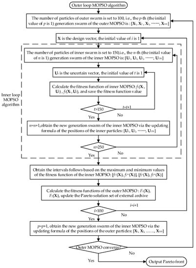
Figure 3.
Flow chart of double-loop multi-objective particle swarm optimization (DL-MOPSO) algorithm.
The steps of the algorithm are as follows:
- (1)
- Set the number of the swarm particles as 100 for the outer loop MOPSO algorithm, that is, the pth generation outer swarm is [X1, X2, …, X100] (the initial value of p is 1);
- (2)
- Select the design vector (the initial value of is 1) in the pth generation outer swarm and enter into the inner-loop MOPSO algorithm;
- (3)
- Set the number of the swarm particles as 150 for the inner loop MOPSO algorithm, that is, the inner swarm is [U1, U2, …, U150] for the nth generation (the initial value of n is 1);
- (4)
- Substituting the uncertainty vector (the initial value of t is 1) in the nth generation inner swarm and the design vector into Equations (13) and (14), calculate the fitness function of the inner-loop MOPSO algorithm and save its value;
- (5)
- If , jump to Step (6); otherwise, , jump to Step (4);
- (6)
- ; from the position-updating formula of the inner particles, a new inner swarm is derived: [U1, U2, …, U150];
- (7)
- If , jump to Step (8); otherwise, jump to Step (3);
- (8)
- According to the maximum and minimum values of the fitness function of the inner-loop MOPSO algorithm already saved, output the intervals , to the outer-loop MOPSO algorithm for developing the fitness function of the outer MOPSO;
- (9)
- Calculate the fitness function of the outer loop MOPSO algorithm via Equations (17) and (18) to update the Pareto solution set in the external archival set of the outer-loop MOPSO algorithm. There are no more than 100 Pareto solutions in the solution set;
- (10)
- If , jump to Step (11); otherwise, let and jump to Step (2);
- (11)
- ; get a new outer swarm based on the position-updating formula of the outer particles: [X1, X2, …, X100];
- (12)
- If the outer-loop MOPSO algorithm satisfies the convergence condition, jump to Step (13); otherwise, jump to Step (1). When one of the following two conditions is satisfied, it is determined as convergence: I. The maximum number of iterations is achieved. II. After 30 continuous iterations, there is no new Pareto solution saved in the external archive set;
- (13)
- Output the front of the Pareto solution set.
After performing the DL-MOPSO algorithm, the Pareto solution sets at different spring heights are illustrated in Figure 4, where F1 and F2 are values of and expressed in Equations (17) and (18).
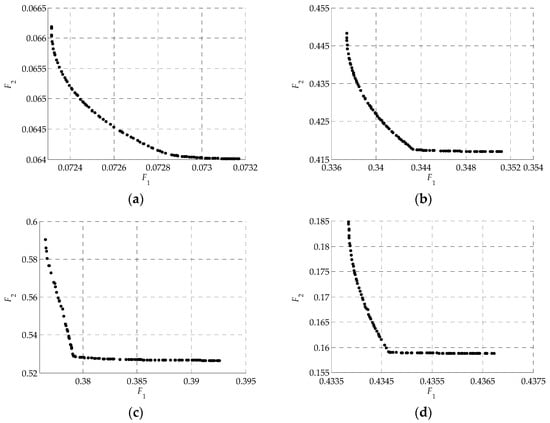
Figure 4.
(a) Pareto solution set of H0; (b) Pareto solution set of H1; (c) Pareto solution set of H2; and (d) Pareto solution set of H3.
It is shown from Figure 4 that the DLSC and a are contradictory in the Pareto solution set. In order to select the optimal solution, the TOPSIS (Technique for Order Preference by Similarity to an Ideal Solution) method was used to get the optimal solutions of Xi [39], which are shown in Table 4.
Table 4.
Optimal geometric parameters of longitudinal-connected suspension at different spring heights based on the DL-MOPSO algorithm.
It is indicated from Table 4 that the optimal value of x1 (inner diameter of air line) is constant, while the optimal value of x2 (inner diameter of connector) changes with spring height. The change of the inside area of the connectors can be realized through control valves placed in the connectors to change their inside areas, along with the control of spring height.
In previous studies, two traditional types of longitudinal connections were usually used to connect the passive air suspensions on the same side: Type 1 (three 6.5 mm inside diameter connectors connecting a 6.5 mm inside diameter air line) and Type 2 (three 20 mm inside diameter connectors connecting a 50 mm inside diameter air line) [8]. The longitudinal connection with the optimal parameters is defined as Type 3.
6. Analysis of Optimization Results
In order to compare the performances of three types of connections (Type 1, Type 2, and Type 3), according to the range of the uncertain variables at the four spring heights shown in Table 2, the upper bound, middle value, and lower bound of each uncertain variable were selected as driving conditions 1–3, respectively. Comparisons were made among the three types of connections in the three driving conditions at each spring height, respectively. The results are shown in Table 5, Table 6, Table 7 and Table 8.
Table 5.
Comparisons among the three types of connections at the spring height of H0.
Table 6.
Comparisons among the three types of connections at the spring height of H1.
Table 7.
Comparisons among the three types of connections at the spring height of H2.
Table 8.
Comparisons among the three types of connections at the spring height of H3.
Based on Table 5, Table 6, Table 7 and Table 8, the optimization rates of Type 3 relative to Type 1 and Type 2 are illustrated in Figure 5. The optimization rate refers to the reduction ratio of DLSC and a using Type 3 connection, compared with using Type 1 and Type 2 connections. As shown in the figures, with respect to different spring heights and driving conditions, compared with the two traditional types, the optimization rate of a is 1.44~35.1%. The DLSC optimization rate reaches 0.44~20.75% in most cases, except for a slight increase (1.04%) relative to Type 1 longitudinal connection in Condition 2, when the spring height is H0. The reason for the increase of DLSC is that the optimization in this paper targets the minimum evaluation functions corresponding to the variation intervals of DLSC and a when the uncertain variable is changing, so the optimization effect may not be desirable when the uncertain variables take a certain set of values. However, in most driving conditions, the DL-MOPSO algorithm proposed in this paper can guarantee the comprehensive driving performance of the semi-trailer with longitudinal-connected air suspensions.
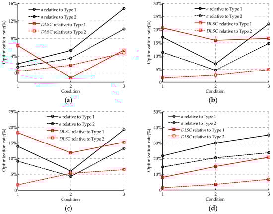
Figure 5.
(a) Optimization rate of Type 3 relative to Type 1 and Type 2 at H0; (b) Optimization rate of Type 3 relative to Type 1 and Type 2 at H1; (c) Optimization rate of Type 3 relative to Type 1 and Type 2 at H2; (d) Optimization rate of Type 3 relative to Type 1 and Type 2 at H3.
From an engineering point of view, favourable dynamic load-sharing (low DLSC) can ensure the equalization of the axle group load across all wheels/axles, which has at least two advantages: (a) it reduces the possibility of a tire bursting as well as enhancing the maneuverability and stability of the vehicle; and (b) it alleviates the rutting and fatigue that contributes to pavement damage. Desirable ride comfort (low α) decreases the possibility of damage to goods during transportation and thus reduces transportation costs.
7. Conclusions
In order to improve the load-sharing and riding comfort of longitudinal-connected air suspension, a nonlinear model for a 5-DOF tri-axle semi-trailer with longitudinal-connected air suspension was formulated based on fluid mechanics and thermodynamics. The strategy for controlling the height of the longitudinal-connected air suspensions was designed according to road roughness, driving speed, and vehicle load. Then, for various spring heights of the semi-trailer, the SVR algorithm was adopted to fit the relational models of the load-sharing and the ride comfort indices, respectively, with the changes in driving conditions and suspension parameters. The coefficient of determination indicated that the goodness of fit of the fitting models was desirable.
A DL-MOPSO algorithm was proposed to tackle the uncertainty of the road roughness, driving speed, and vehicle load in the optimization of geometric parameters of the longitudinal-connected air suspension. In the DL-MOPSO algorithm, the inner-loop algorithm is utilized to calculate the interval range of the target function when the uncertain variable is changing, while the outer-loop algorithm is used for global optimization of the inner diameters of the optimal air lines and connectors. The optimal inner diameter of air lines is a constant value at various spring heights. However, the optimal inner diameter of the connector changes with spring height. This can be realized through the control of valves placed in the connectors to change their inside areas, along with the control of spring height.
Compared with the two traditional suspensions, the optimization rates of DLSC and a are −1.04~20.75% and 1.44~35.1%, respectively. The reason for the slight increase of DLSC in Condition 2 when the spring height is H0 is that the optimization in this paper targets the minimum evaluation function corresponding to the DLSC and a variation interval when the uncertain variable is changing, so the optimization effect may not be good when the uncertain variable takes a certain set of values. Generally, the DL-MOPSO algorithm proposed in this paper can guarantee the comprehensive driving performance of the semi-trailer with longitudinal-connected air suspension and is robust to change in driving conditions. Based on the signals measured from the suspension height sensors, the proposed method can be realized through integrated control of inflation/deflation valves of air suspensions, as well as the valves inside connectors and air lines.
Author Contributions
Conceptualization, Y.C. and W.H.; Methodology, H.P.; Software, S.H.; Validation, L.D.; Formal Analysis, J.H. and H.P.; Investigation, L.D.; Resources, Q.S.; Data Curation, Q.W.; Writing—Original Draft Preparation, Y.C. and S.H.; Writing—Review & Editing, Q.S. and J.H.; Visualization, Q.W.; Supervision, Y.C.
Acknowledgments
This research was funded by the National Natural Science Foundation of China (grant number 51305117) and the Fundamental Research Funds for the Central Universities (grant number JZ2017HGTB0212). And the APC was funded by the National Natural Science Foundation of China (grant number 51305117).
Conflicts of Interest
The authors declare no conflict of interest.
References
- Gong, B.; Guo, X.; Hu, S.; Xu, L. Ride comfort optimization of a multi-axle heavy motorized wheel dump truck based on virtual and real prototype experiment integrated Kriging model. Adv. Mech. Eng. 2015, 7, 1–15. [Google Scholar] [CrossRef]
- Trigell, A.S.; Rothhämel, M.; Pauwelussen, J.; Kural, K. Advanced vehicle dynamics of heavy trucks with the perspective of road safety. Veh. Syst. Dyn. 2017, 55, 1–46. [Google Scholar] [CrossRef]
- Li, J.; He, J.; Li, X. Multi-objective optimization of vehicle air suspension based on simulink-mfile mixed programming. Appl. Mech. Mater. 2014, 509, 63–69. [Google Scholar] [CrossRef]
- Davis, L.E.; Bunker, J.M. Load-sharing in heavy vehicle suspensions: new metrics for old. In Proceedings of the Second Infrastructure Theme Postgraduate Conference, Brisbane, Australia, 12 November 2008. [Google Scholar]
- Cebon, D. Vehicle-Generated Road Damage: A Review. Veh. Syst. Dyn. 1989, 18, 107–150. [Google Scholar] [CrossRef]
- Sweatman, P.F. A Study of Dynamic Wheel Forces in Axle Group Suspensions of Heavy Vehicles; Technical Report; Australian Road Research Board (ARRB): Vermont South, Victoria, Australia, 1983.
- Organisation for Economic Cooperation and Development, Scientific Expert Group. Dynamic Loading of Pavements; Technical Report; OECD Road Transport Research: Paris, France, 1992. [Google Scholar]
- Davis, L.; Bunker, J. Altering heavy vehicle air suspension dynamic forces by modifying air lines. Int. J. Heavy Veh. Syst. 2011, 18, 1–17. [Google Scholar] [CrossRef]
- Cantieni, R.; Krebs, W.; Heywood, R. Dynamic Interaction between Vehicles and Infrastruction Experiment (Divine); Technical Report; Organisation for Economic Co-operation and Development (OECD): Paris, France, 1998. [Google Scholar]
- Roaduser Systems Pty Ltd. Stability and On-Road Performance of Multi-Combination Vehicles with Air Suspensions Systems Project. Overarching Report; Technical Report; National Road Transport Commission: Canberra, Australia, 2005.
- Xu, X.; Zou, N.; Chen, L.; Cui, X. Modelling and analysis of parallel-interlinked air suspension system based on a transfer characterisation. Int. J. Heavy Veh. Syst. 2016, 12, 1–23. [Google Scholar] [CrossRef]
- Li, Z.; Ju, L.; Jiang, H.; Xu, X.; Li, M. Experimental and simulation study on the vibration isolation and torsion elimination performances of interconnected air suspensions. Proc. Inst. Mech. Eng. Part D J. Automob. Eng. 2016, 230, 679–691. [Google Scholar] [CrossRef]
- Li, Z.; Ju, L.; Jiang, H.; Xu, X. Imitated skyhook control of a vehicle laterally interconnected air suspension. Int. J. Veh. Des. 2017, 74, 204–230. [Google Scholar] [CrossRef]
- Cebon, D.; Roebuck, R.L.; Dale, S.G. Optimal control of a semi-active tri-axle lorry suspension. Veh. Syst. Dyn. 2006, 44 (Suppl. 1), 892–903. [Google Scholar]
- Kat, C.-J.; Els, P.S. Interconnected air spring model. Math. Model. Syst. 2009, 15, 353–370. [Google Scholar] [CrossRef]
- Chen, Y.; He, J.; King, M.; Chen, W.; Zhang, W. Effect of driving conditions and suspension parameters on dynamic load-sharing of longitudinal-connected air suspensions. Sci. Chin. 2013, 56, 666–676. [Google Scholar] [CrossRef]
- Chen, Y.; He, J.; King, M.; Chen, W.; Wang, C.; Zhang, W. Model Development and Dynamic Load-Sharing Analysis of Longitudinal-Connected Air Suspensions. Stroj. Vestn. 2013, 59, 14–24. [Google Scholar] [CrossRef]
- Zhu, H.; Yang, J.; Zhang, Y. Modeling and optimization for pneumatically pitch-interconnected suspensions of a vehicle. J. Sound Vib. 2018, 432, 290–309. [Google Scholar] [CrossRef]
- Abbasa, M.; Bellahcene, F. Cutting plane method for multiple objective stochastic integer linear programming. Eur. J. Oper. Res. 2006, 168, 967–984. [Google Scholar] [CrossRef]
- Liu, B.; Iwamura, K. Fuzzy programming with fuzzy decisions and fuzzy simulation-based genetic algorithm. Fuzzy Sets Syst. 2001, 122, 253–262. [Google Scholar] [CrossRef]
- Moore, R.E. Methods and Applications of Interval Analysis; The Society for Industrial and Applied Mathematics: Philadelphia, PA, USA, 1979. [Google Scholar]
- Ishibuchi, H.; Tanaka, H. Multiobjective programming in optimization of the interval objective function. Eur. J. Oper. Res. 1990, 48, 219–225. [Google Scholar] [CrossRef]
- Bai, L.; Li, F.; Cui, H.; Jiang, T.; Sun, H.; Zhu, J. Interval optimization based operating strategy for gas-electricity integrated energy systems considering demand response and wind uncertainty. Appl. Energy 2016, 167, 270–279. [Google Scholar] [CrossRef]
- Feng, Y.; Zhang, Z.; Tian, G.; Lv, Z.; Tian, S.; Jia, H. Data-driven accurate design of variable blank holder force in sheet forming under interval uncertainty using sequential approximate multi-objective optimization. Future Gener. Comput. Syst. 2018, 86, 1242–1250. [Google Scholar] [CrossRef]
- Allotta, B.; Pugi, L.; Colla, V.; Bartolini, F.; Cangioli, F. Design and optimization of a semi-active suspension system for railway applications. J. Mod. Transp. 2011, 19, 223–232. [Google Scholar] [CrossRef]
- Ma, Y.; Xu, T.; Qian, F. Machine tool support multi-objective robustness design under uncertainties. Comput. Integr. Manuf. Syst. 2017, 23, 482–487. [Google Scholar]
- Cheng, J.; Duan, G.F.; Liu, Z.Y.; Li, X.G.; Feng, Y.X.; Chen, X.H. Interval multiobjective optimization of structures based on radial basis function, interval analysis, and NSGA-II. J. Zhejiang Univ. Sci. A 2014, 15, 774–788. [Google Scholar] [CrossRef]
- Coello, C.A.C.; Pulido, G.T.; Lechuga, M.S. Handling multiple objectives with particle swarm optimization. IEEE Trans. Evol. Comput. 2004, 8, 256–279. [Google Scholar] [CrossRef]
- Raquel, C.R.; Naval, P.C., Jr. An effective use of crowding distance in multiobjective particle swarm optimization. In Proceedings of the 7th Annual Conference on Genetic and Evolutionary Computation, Washington, DC, USA, 25–29 June 2005; pp. 257–264. [Google Scholar]
- Pugi, L.; Galardi, E.; Carcasci, C.; Rindi, A.; Lucchesi, N. Preliminary design and validation of a real time model for hardware in the loop testing of bypass valve actuation system. Energy Convers. Manag. 2015, 92, 366–384. [Google Scholar] [CrossRef]
- Davis, L.E.; Bunker, J.M. Suspension Testing of 3 Heavy Vehicles—Dynamic Wheel Force Analysis; Department of Main Roads-Queensland Government: Brisbane, Australia, 2009.
- De Pont, J. Assessing Heavy Vehicle Suspensions for Road Wear; California Transit Association: Wellington, New Zealand, 1997. [Google Scholar]
- Chen, Y.K.; He, J.; King, M.; Chen, W.W.; Zhang, W.H. Stiffness-dam;ping matching method of an ECAS system based on LQG control. J. Cent. South Univ. 2014, 21, 439–446. [Google Scholar] [CrossRef]
- Yu, Z. Automobile Theory, 5th ed.; China Machine Press: Beijing, China, 2009; pp. 203–251. [Google Scholar]
- Thite, A.N.; Coleman, F.; Doody, M.; Fisher, N. Experimentally validated dynamic results of a relaxation-type quarter car suspension with an adjustable damper. J. Low Freq. Noise Vib. Act. Control 2017, 36, 148–159. [Google Scholar] [CrossRef]
- Anderson, M.J.; Whitcomb, P.J. Design of Experiments; John Wiley & Sons: Hoboken, NJ, USA, 2000. [Google Scholar]
- Chang, C.C.; Lin, C.J. LIBSVM: A Library for Support Vector Machines; Association for Computing Machinery: Washington, DC, USA, 2011; pp. 1–27. [Google Scholar]
- Hu, W.; Gray, G.; Zhang, X. Multiobjective Particle Swarm Optimization Based on Pareto Entropy. J. Softw. 2014, 25, 1025–1050. [Google Scholar]
- Shojaeefard, M.H.; Khalkhali, A.; Faghihian, H.; Dahmardeh, M. Optimal platform design using non-dominated sorting genetic algorithm II and technique for order of preference by similarity to ideal solution; application to automotive suspension system. Eng. Optim. 2018, 50, 471–482. [Google Scholar] [CrossRef]
© 2018 by the authors. Licensee MDPI, Basel, Switzerland. This article is an open access article distributed under the terms and conditions of the Creative Commons Attribution (CC BY) license (http://creativecommons.org/licenses/by/4.0/).