Numerical Research on the Mixture Mechanism of Polluted and Fresh Air at the Staggered Tunnel Portals

Abstract

In longitudinal ventilation, circulating air is formed in portals for closely spaced twin tunnels, which causes mixing between the polluted air exhausted from one tunnel and the fresh air flow of another tunnel, thus leading to the rising costs of ventilation system construction and operation. In this study, for the closely spaced tunnel with staggered inlet and outlet, the computational fluid dynamics (CFD) numerical simulation method was adopted to reveal flow characteristics of the circulating air as well as variation rules of the circulating air mixing ratio φ_c with tunnel structure and operation parameters. Results show that both reducing inlet air velocity and increasing outlet air velocity and lateral distance can reduce the impact of the negative-pressure zone at the tunnel entrance on the jet flow structure at the tunnel exit, thus weakening the circulating air. When the inlet is placed behind or aligned with the outlet (staggered distance ∆l ≤ 0), φ_c will increase linearly along with the increase of staggered distance; when the inlet is placed before the outlet (∆l > 0), φ_c will first increase and then decrease with the increase of staggered distance. An expression to predict circulating air mixing ratio was created by sections. The predictions show a good correlation with the measurements and indicate that the front slope gradient of the tunnel portal is also one of the factors affecting the circulating air mixing ratio.

1. Introduction

With the current state of economic development and increasing transportation demands, more and more tunnels are being put into construction [1]. Tunnels can be referred to as a special type of semi-enclosed passageway. When vehicles pass through the tunnels, the exhaust gas will accumulate and therefore increase the concentration of harmful substances such as carbon monoxide, nitrogen oxides, and particulates, which will deteriorate the operating environment in the tunnel [2,3] and even cause a series of health problems such as dyspnea and cardiovascular diseases [4,5]. Usually, ventilation equipment is adopted to dilute the pollutant concentration in the tunnels [6,7,8]. In recent years, due to being restricted by landforms and architectural patterns, more and more twin tunnels with small spacing are being constructed [9,10]. During the operation of this kind of tunnel, not only do the pollutants of the outlet tunnel influence the local environment of the tunnel exit [11], but the pollutants also mix with new incoming air at the adjacent inlet to form circulating air, consequently intensifying the pollution level at the internal environment of the inlet tunnel and resulting in increasing costs of ventilation system construction and operation.

At present, many scholars have studied the circulating air at the portals of twin tunnels with small spacing. Through three-dimensional numerical simulations and field tests, Chen et al. [12] presented how the mixed volume of pollutants correlated with the tunnel spacing and airflow velocity at the inlet/outlet. They concluded that the mixed proportion of the polluted airflow could be reduced by increasing the outlet air velocity and lateral distance of the tunnel portals as well as decreasing the inlet air velocity. Through a model test, Tan et al. [13] established a testing ventilation system of a close tunnel model and conducted a series of experiments. The results showed that when inlet and outlet airflow velocity were equal, the mixed volume of pollutants was barely influenced by the airflow velocity but would decrease with the increase of the tunnel spacing. Based on the experimental data, they also obtained the quantitative relationship between the mixed volume of pollutants and inlet/outlet airflow velocity and tunnel spacing. Through numerical simulation, Yang et al. [14] further analyzed the influence of ambient wind on the pollutant diffusion at the tunnel portals. They concluded that under adverse ambient wind conditions, the degree of influence of the exhaust pollutant at outlet air tunnel portal on the inlet air tunnel lessened as the environmental air slowed down. According to previous findings [12,15], the circulating air can be effectively weakened by establishing midboards, green belts, or building horizontal ventilation tunnels.

It should be noted that many closely spaced twin tunnels with staggered inlet and outlet exist due to landform restrictions. For instance, for the Baziling Tunnel in the Hurong highway, the inlet is about 5 m behind the outlet. At the north opening of the #1 tunnel of the Zizhi Tunnel in Hangzhou, the inlet is about 19 m before the outlet; at the south opening of the #3 tunnel, the inlet is about 44 m before the outlet. The circulating air can be effectively influenced by staggering the inlet and outlet air tunnel portals. For example, by increasing the length of outlet air tunnel portal and repositioning it at a point 5 m away from the inlet, the proportion of polluted airflow mixed with fresh airflow will be lower than 5% [13]. However, previous research mostly focused on closely spaced twin tunnels with aligned inlet and outlet air tunnel portals, and studies relating to the circulating air of the staggered inlet and outlet are still inadequate.

The present research focuses on closely spaced twin tunnels with staggered inlet and outlet and uses the computational fluid dynamics (CFD) simulation technique to analyze the characteristics of circulating air, as well as to acquire the variation of the intake volume of pollutants caused by the circulating wind with the airflow velocity, tunnel spacing, and staggered distance. Based on these results, an expression for predicting the mixed proportion of the polluted airflow is suggested, which can provide an important reference for the economic and environmental protection evaluation of closely spaced twin tunnels design.

2. Mathematical Model

2.1. Governing Equations and Numerical Algorithm

The airflow and pollutant diffusion at the tunnel portals are influenced by various factors. In order to explore the inherent law of the flow field, the following assumptions are put forward in this paper: (1) vehicles are regarded as external and accidental factors, with no influence on the airflow; (2) natural wind is regarded as the external boundary at a velocity of 0 m·s⁻¹; (3) the airflow temperature at all inlet and outlet boundaries is 300 K, without any volume source; (4) as the pollutant components are scalar with similar distributional patterns, CO concentration distribution is used to represent the pollutant diffusion.

The airflow velocity at the portals is much slower than the sound velocity, so it can be regarded as a steady turbulent flow of incompressible fluid [14]. This paper calculated the airflow at the inlet and outlet based on the Standard k-ε turbulence model. The pollutant diffusion was described through the species transport equation. The buoyancy-driven effects caused by density changes due to varied components of mixed gas were not considered. The transport equations of the turbulent kinetic energy k and turbulent dissipation rate ε in the Standard k-ε turbulence model and species transport equation are shown in Equations (1)–(3).

$$\frac{\partial }{\partial x_i}\left(\rho k{u}_i\right)=\frac{\partial }{\partial x_j}\left[\left(\mu +\frac{{\mu }_t}{{\sigma }_k}\right)\frac{\partial k}{\partial x_j}\right]+G_k-\rho \epsilon$$

(1)

$$\frac{\partial }{\partial x_i}\left(\rho \epsilon u_i\right)=\frac{\partial }{\partial x_j}\left[\left(\mu +\frac{{\mu }_t}{{\sigma }_{\epsilon }}\right)\frac{\partial \epsilon }{\partial x_j}\right]+C_{1\epsilon }\frac{\epsilon }{k}{G}_k-C_{2\epsilon }\rho \frac{{\epsilon }^2}{k}$$

(2)

$$\frac{\partial \left(\rho c_s{u}_i\right)}{\partial x_i}=\frac{\partial }{\partial x_j}\left[D_s\frac{\partial \left(\rho c_s\right)}{\partial x_j}\right]+S_s$$

(3)

In the above formula, both the values of i and j range from 1 to 3; x_i represents the coordinate components; ρ, μ, ν, and u are the mass density of air, turbulent viscosity, coefficient of kinematic viscosity, and air velocity; c_s refers to the volume density of s; D_s refers to the diffusion coefficient of s; S_s refers to the quality of s generated from the chemical reaction in unit time and volume, namely, the productivity; C_μ, σ_k, σ_ε, C_1ε, C_2ε, and C_3ε are model coefficients that follow the principle of asymptotic proportionality [16], and their values are 0.09, 0.24, 0.15, 1.44, 1.92, and 0.2.

Equations (1)–(3) and the Reynolds-averaged Navier–Stokes equation [17,18] constituted the governing equations for the pollutant diffusion of closely spaced twin tunnels. The finite volume method [19] was used to discretize the governing equations. For the discretization of derivatives, the skewness-corrected linear upwind interpolation scheme (second-order accuracy) was applied to the convective terms, and second-order linear interpolation was used with a nonorthogonal correction scheme for the diffusive terms [20]. The solution of the velocity field and pressure field was conducted through a fully coupled block algorithm. Due to the simultaneous solution of momentum and continuity equations, implicit block coupling of pressure and velocity variables leads to faster convergence with respect to classical, loosely coupled, segregated algorithms of the SIMPLE family of algorithms [21].

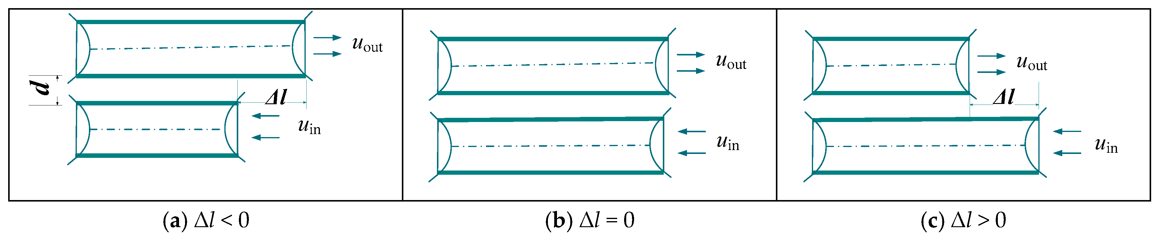
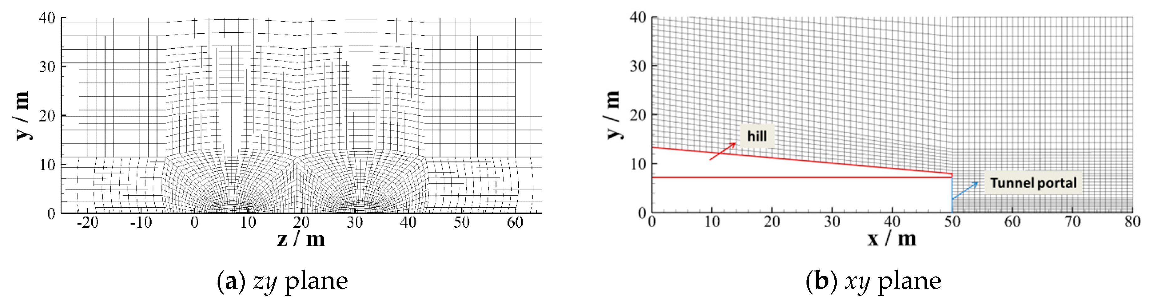
2.2. Computational Geometry, Domain, and Grid

The airflow within about a 450-m length, 200-m width, and 50-m height range outside the tunnel portals was adopted to simulate the pollutant diffusion. The tunnel section resembled the shape of a horseshoe. The two-lane and three-lane tunnels were considered separately, and the hydraulic diameters D were 6.1 and 8.6 m, respectively. In reference to a certain tunnel project, the front slope gradient of the tunnel portal was 15°. The lateral distance of inlet and outlet d was set within the range of 5–20 m at 2.5-m intervals. The staggered distance Δl was from −10 to 320 m at 5 m intervals. If Δl < 0, the inlet would be positioned behind the outlet as shown in Figure 1a; if Δl = 0, the outlet and inlet would be aligned as shown in Figure 1b; if Δl > 0, the inlet would be positioned in front of the outlet as shown in Figure 1c.

The whole domain was meshed by nonuniform hexahedral grids using the professional mesh generation software ICEM-CFD17.2 (ANSYS Inc. Pittsburgh, PA, USA, 2016), and the areas near the inlet and outlet were locally refined to ensure calculation efficiency, accuracy, and reliability. Figure 2 shows the grid map of a three-lane tunnel with a lateral distance d = 10 m.

2.3. Grid Dependence Study

Grid density exerts a great impact on the numerical simulation results. When the grid number is relatively small, the dispersion error will be very large; when the grid number is large, not only will the rounding error increase, but the calculation quantity will increase as well. Figure 3 shows that the velocity profile in the symmetry plane is 30 m away from the outlet under different grid orders of 0.08 × 10⁶, 0.47 × 10⁶, 1.05 × 10⁶, and 5.78 × 10⁶. It can be seen that the number of grids has a great effect on the velocity profile. When the number of grids reaches 1.05 × 10⁶, the velocity profile will no longer change with the increase of grid number.

2.4. Boundary Conditions

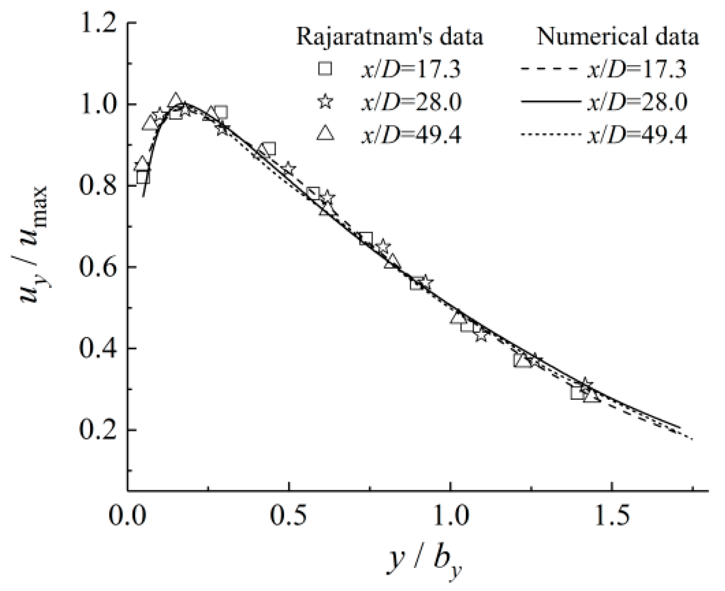
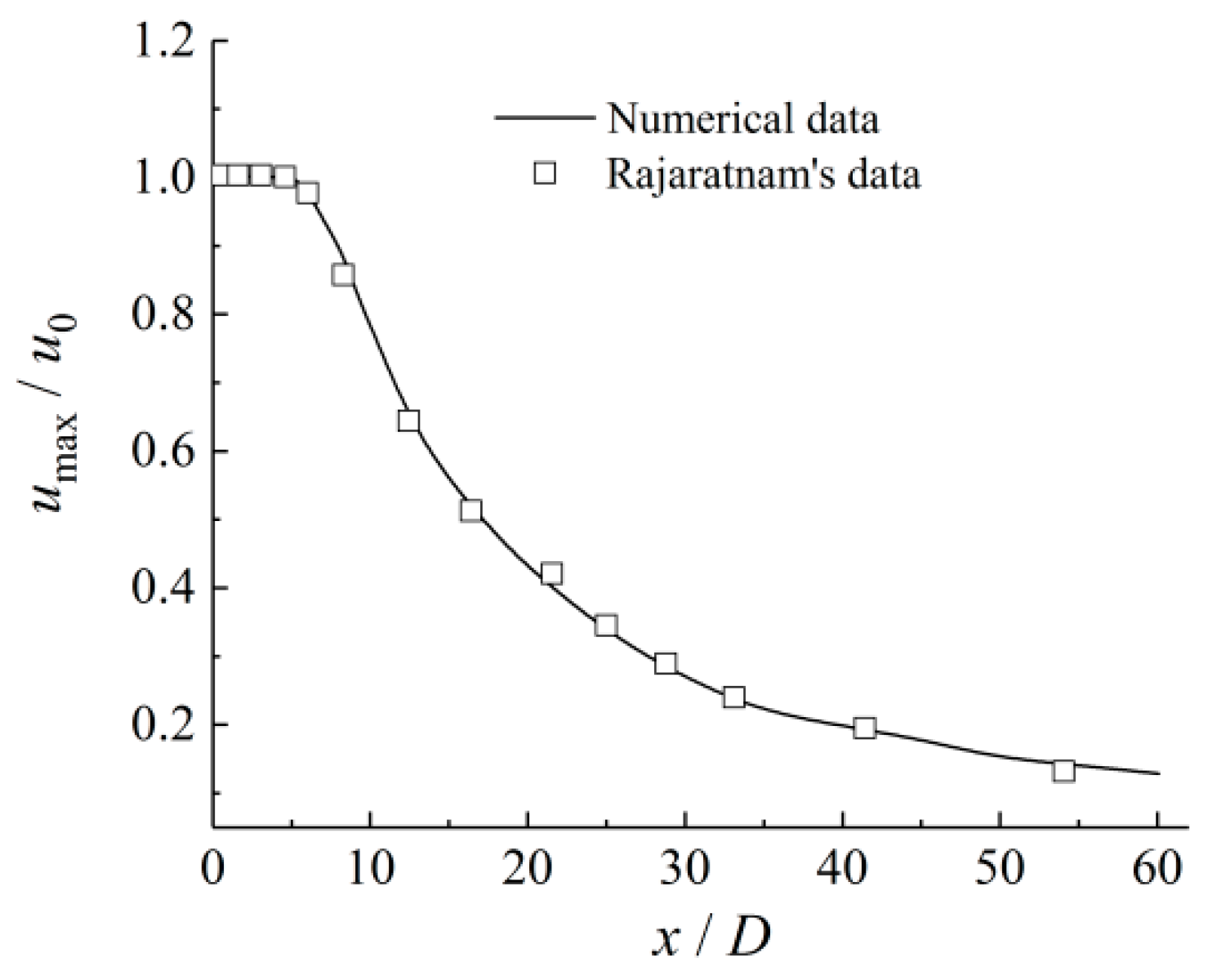
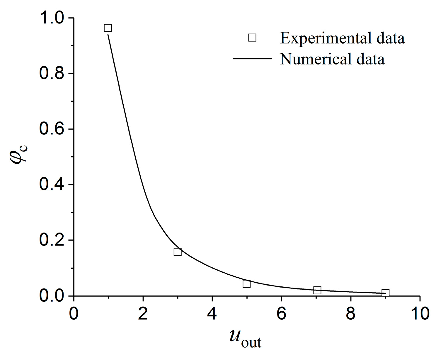
A Neumann boundary condition for pressure was used at the outer boundary of the computational domain. The tunnel walls and pavement were taken as an impenetrable, nonslip boundary. It should be noted that the Standard k-ε model as a turbulence model for high Re numbers is not applicable to the near-wall area where the flowing Re number is low. Therefore, in order to capture the near-wall region’s flow structures, the kqRwallFunction and epsilonWallFunction, also called standard wall functions in OpenFOAM 2.1.1 (OpenCFD Ltd., Bracknell, UK, 2012) [20], were assigned to the turbulence kinetic energy and dissipation rate, respectively. Using the wall function allowed us to locate the first point adjacent to the wall in the logarithmic law instead of the sublayer. The calculated y+ value should be distributed between 30 and 300 in all simulations. According to y+, the distance of the near-wall node to the solid surface was calculated, which was also corrected continuously through computational simulation. Ultimately, it could be determined that y+ can be ensured between 32 and 132 under all computation conditions when the first layer grid thickness was 0.018 m.

The tunnel inlet and outlet adopted the Dirichlet boundary condition. According to the ventilation conditions of the actual tunnel and the possible working conditions during the project’s operational phase, calculations were separately conducted with respect to the following working conditions: at outlet air velocity u_out of 1.5 m·s⁻¹, 3.0 m·s⁻¹, 4.5 m·s⁻¹, 6.0 m·s⁻¹, and 7.5 m·s⁻¹; and inlet air velocity u_in of 1.5 m·s⁻¹, 3.0 m·s⁻¹, 4.5 m·s⁻¹, 6.0 m·s⁻¹, and 7.5 m·s⁻¹. The numerical computations in this study were conducted by OpenFOAM, an opensource CFD code with flexible and extendable C++ libraries.

2.5. Validation

The discharge of the tunnel outlet pollutants was horizontal and was constrained by the ground boundaries, all of which constituted a typical three-dimensional wall jet problem. Rajaratnam [22] conducted a series of wall jet experiments in a semi-infinite three-dimensional space. This paper attempted to verify the numerical model of the airflow by utilizing the experimental findings of the jet flow over the circular nozzle. The diameter D of the circular nozzle was 0.00953 m and the jet flow outlet speed u₀ was 7.42 m·s⁻¹. The comparison between the numerical results and the measured values is shown in Figure 4 and Figure 5, which respectively show the decay of nondimensional maximum velocity u_max in the symmetry plane of the three-dimensional wall jet, and the dimensionless velocity profiles at the plane of symmetry at distances x = 0.165, 0.267, and 0.470 m from the jet flow outlet. In Figure 5, u_y represents the speed at the height y above the ground, and b_y is the length scale of the plane of symmetry [23]. It shows that CFD simulation results are consistent with the trend of the test data, with a maximum error of only 5.2%.

In addition to the above, this paper also used the scale model test results of the circulating air in closely spaced twin tunnels in the existing literature [13] to verify the species transport model. The scale model was 10-m long, and the section was a semicircle with a radius of 0.5 m. The lateral distance between the portals d = 4 m, and the front slope of the tunnel portal was perpendicular to the ground. The outlet air velocity u_in was 3 m·s⁻¹ and the air velocity u_out was 1 m·s⁻¹, 3 m·s⁻¹, 5 m·s⁻¹, 7 m·s⁻¹, and 9 m·s⁻¹, respectively. The comparison between the numerical simulation and the scale test results is shown in Figure 6. Results show that change patterns are roughly consistent, with a maximum error of only 5.5%, which indicates that the mathematical model adopted by this paper demonstrates a high degree of accuracy and reliability and is suitable for calculating and simulating the circulating air at tunnel portals.

3. Numerical Simulation Results and Discussions

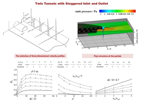
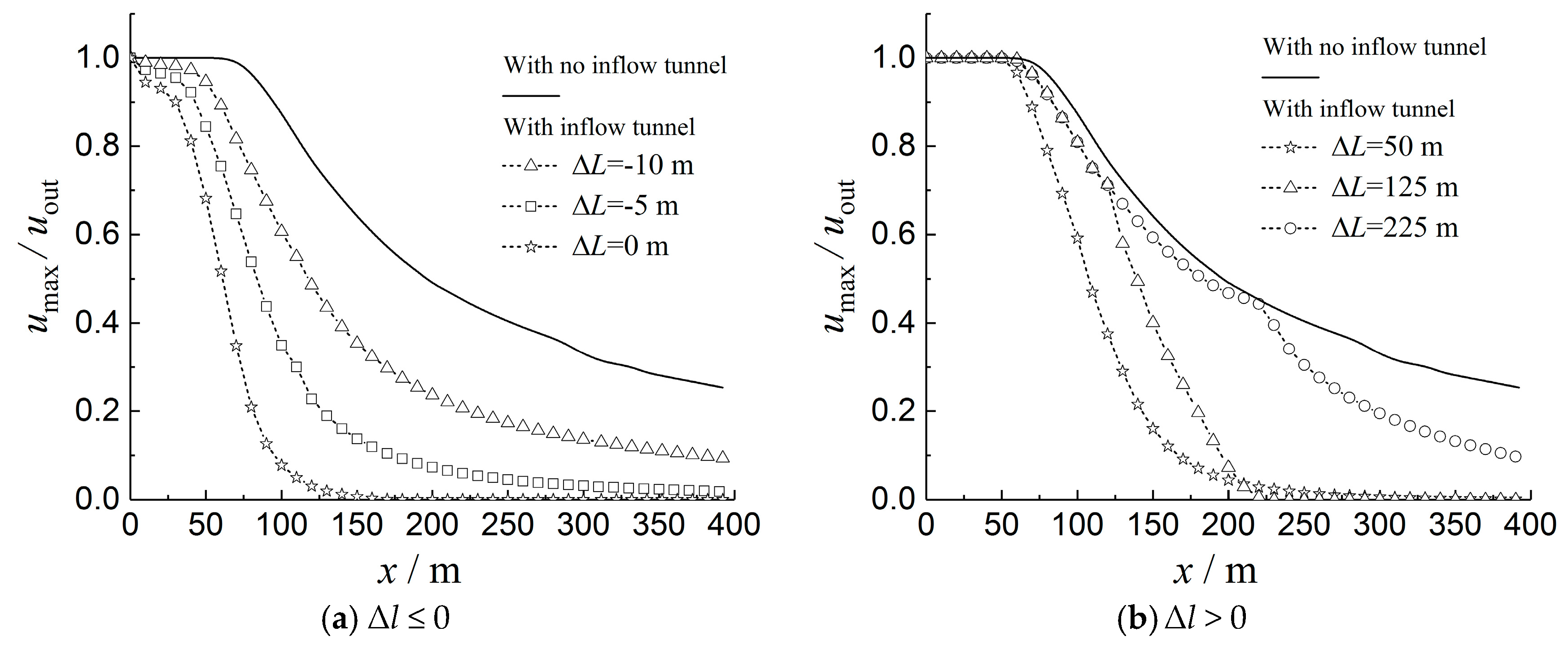
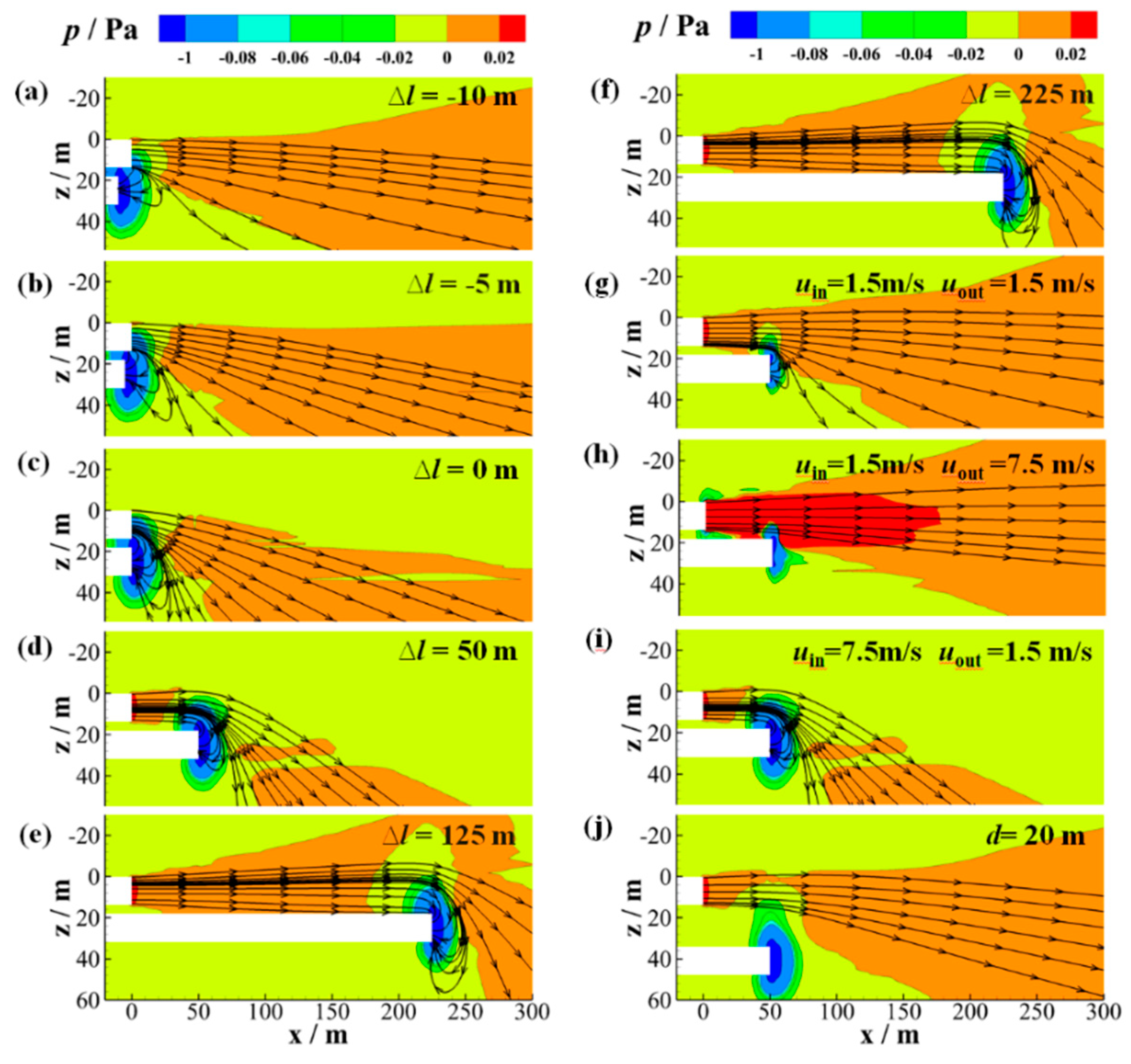
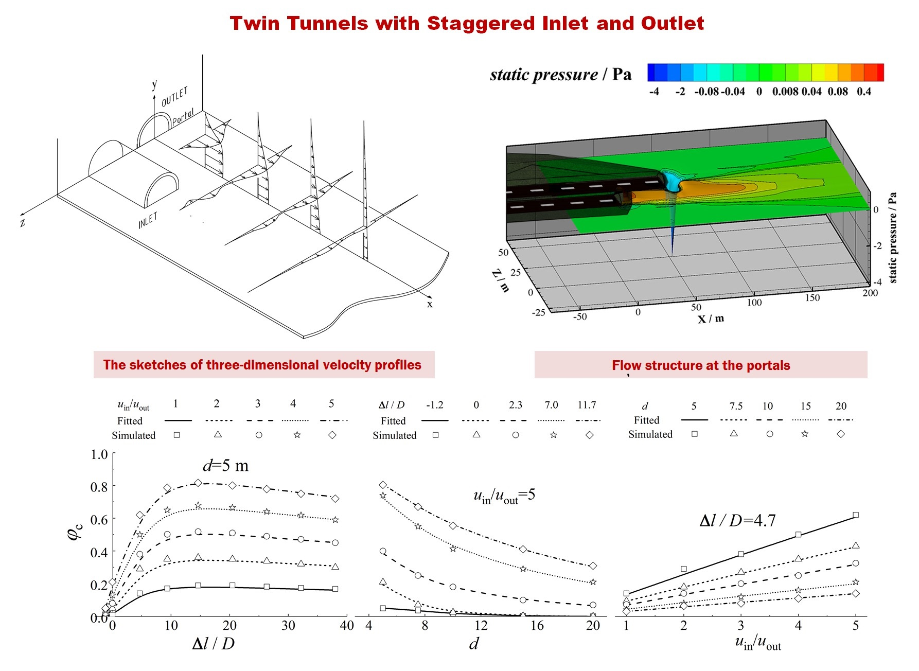
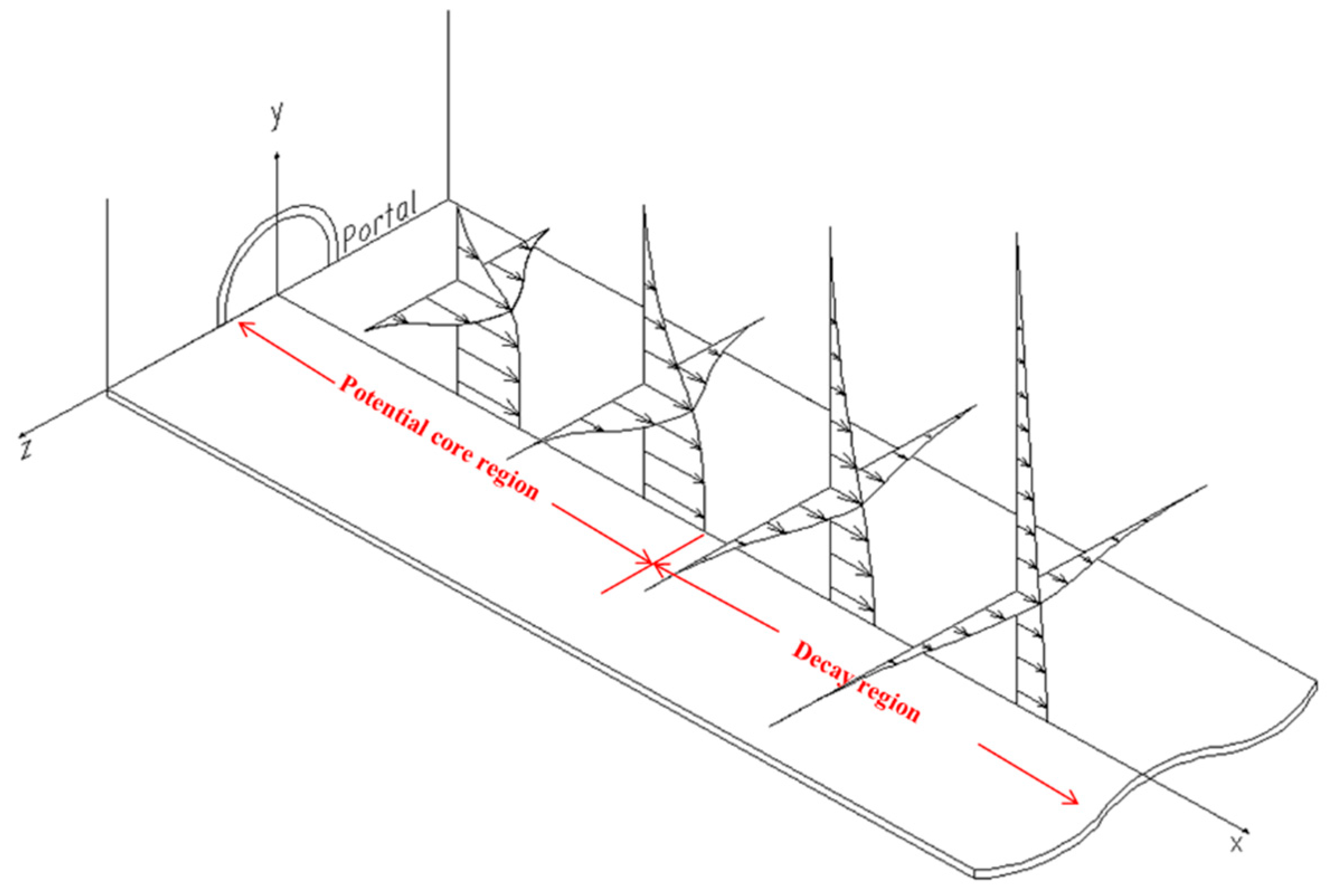
3.1. Flow Characteristic

Figure 7 depicts the sketches of three-dimensional velocity profiles of jet flow at a three-lane tunnel exit. It can be observed that after the air is pushed out from the tunnel exit, due to the lateral fluctuation on the turbulence, the moving wind exchanges momentum with its surrounding stagnant air and drives the surrounding air molecules to move to produce an entrainment effect, thus continuously expanding the jet flow cross-section area. The three-dimensional wall jet can be categorized into the potential core region and decay region, depending on whether the maximum velocity u_max decreases. The decay of nondimensional u_max is shown by the solid line in Figure 8. It can be seen from Figure 7 and Figure 8 that at the potential core region (where x ≤ 60 m), the jet flow fiercely entrains the surrounding air, thereby expanding the jet flow boundary and the flow rate altogether, while reducing the air velocity at the same time, but the u_max remains the same. At the decay region (where x > 60 m), with further development of the jet-flow entrainment and mixing effects, the u_max starts to reduce and the velocity profile also tends to flatten out.

Figure 9 depicts the flow structure at the portals of twin tunnels with small spacing, of which Figure 9a–f show the flow structures under different staggered distance ∆l when the lateral distance of the tunnel portals d = 5 m, inlet air velocity u_in = 7.5 m·s⁻¹, and outlet air velocity u_out = 1.5 m·s⁻¹. When ∆l ≤ 0, the jet flow at the outlet deflects entirely under the influence of the negative-pressure zone at the inlet, as shown in Figure 9a–c. In the meantime, by referring to Figure 8a, it can be noticed that, different from the standard three-dimensional wall jet, the u_max at the moment begins to attenuate when x > 0 (the bigger ∆l is, the quicker the attenuation will be); when ∆l > 0, we can learn from Figure 9d,f and Figure 8b that the jet flow structure at the outlet when x ≤ ∆l and the law of u_max attenuation are both similar to those of the standard three-dimensional wall jet. However, when x > ∆l, the jet flow will deflect under the influence of the negative-pressure zone at the inlet, for which u_max will fall rapidly at a decay rate first increasing and then decreasing along with the increase of ∆l.

Moreover, it can be perceived from the comparison between Figure 9g–h that the bigger u_out is, the bigger the inertia effect of the jet flow will be, and the less vulnerable it will be to the influence of the negative-pressure zone at the inlet and the fuller the jet flow will develop. In this way, the polluted air flowing into the adjacent air-inlet tunnel through the air-exhausting tunnel will be reduced. According to Figure 9g–i, when u_in increases, the bigger the influencing area of the negative-pressure zone is, the bigger the damage caused to the flow structure at the outlet will be, thus resulting in more polluted air flowing into the adjacent air-inlet tunnel through the air-exhausting tunnel. Finally, through comparing Figure 9i with Figure 9j, the bigger d is, the smaller the damage caused by the negative-pressure zone at the inlet to the flow structure at the outlet will be and the fuller the jet flow will develop; when d = 20 m, there is almost no polluted air flowing into the adjacent air-inlet tunnel through the air-exhausting tunnel.

Therefore, it can be concluded that, for closely spaced twin tunnels with staggered inlet and outlet, the air flow discharged from their air-exhausting tunnels will diffuse transversely toward the air-inlet tunnels under the influence of the negative-pressure zone at the inlet, even causing inverse flow and forming the circulating air. Parameters including inlet air velocity u_in, outlet air velocity u_out, lateral distance of the tunnel portals d, and staggered distance ∆l are all important factors influencing the circulating air.

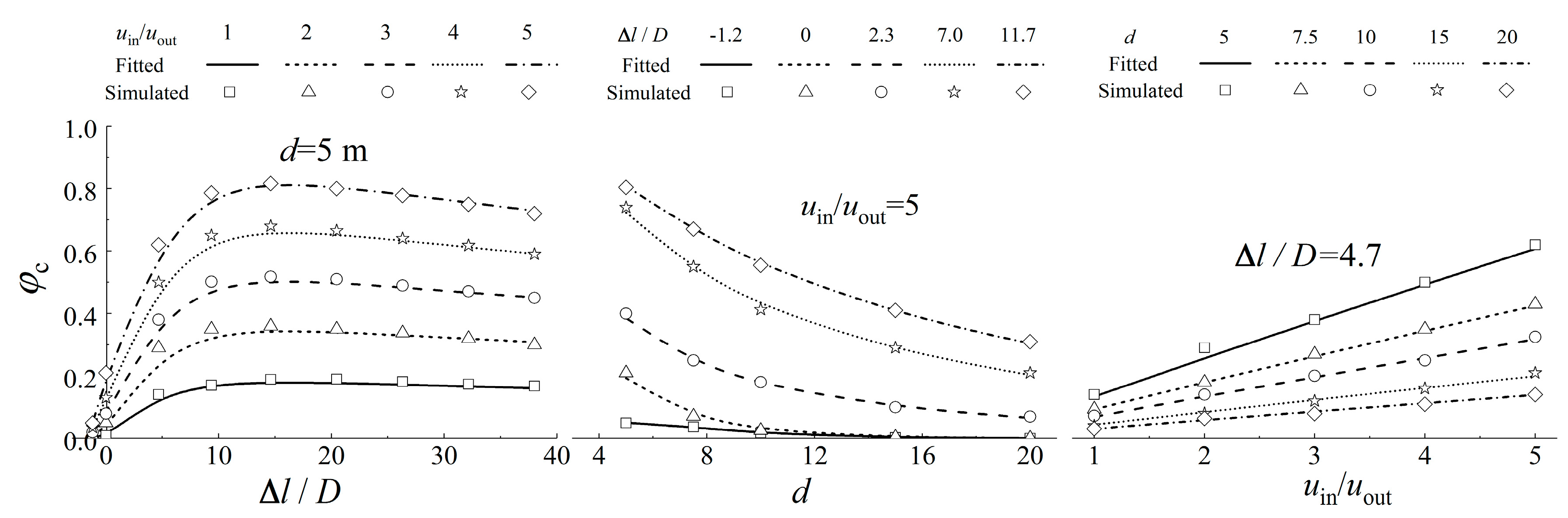
3.2. Variation Characteristics of Circulating Air Mixing Ratio

The circulating air mixing ratio is represented by φ_c = m_c/m_out, where m_c is the amount of pollutants that is carried by the circulating air into the inlet tunnel from the outlet tunnel, and m_out is the total amount of gaseous pollutants discharged from the outlet tunnel. Therefore, it can be perceived that φ_c indicates the degree of impacts of exhaust emission from the outlet tunnel on the inlet tunnel.

3.2.1. The Relationship between Circulating Air Mixing Ratio and the Air Velocity at the Inlet/Outlet

The flow field structure depicted in Figure 9g–i shows that both reducing u_in and increasing u_out can weaken the circulating air. Existing literature [13] has also shown that when u_in = u_out, for closely spaced twin tunnels with aligned inlet and outlet air tunnel portals, φ_c does not change with the change of air velocity value but is related to the ratio of u_in and u_out. Figure 10 shows the variation of φ_c with air velocity at the closely spaced twin tunnels with staggered inlet and outlet. It can be seen that regardless of the relative position of the inlet and outlet, when u_in = u_out, φ_c is not affected by the value of air velocity, and that the variation of φ_c does not exceed 0.3%.

Figure 11 shows the variation of φ_c with u_in/u_out when u_in ≠ u_out. It can be seen that φ_c increases gradually with the increase of u_in/u_out despite the relative position of the inlet and outlet. By further comparing the numerical calculation results of φ_c in the tunnel with aligned inlet and outlet air tunnel portals with the scaled model test results in the literature [13], it can be found that the trend of the simulated data is congruent with the test results in the literature, but the values of the simulation are generally lower than the data in the literature. This is caused by the inconsistency between the front slope gradient (15°) of the tunnel portal for the numerical simulation in this paper and the front slope gradient (90°) of the scaled model in the previous study.

In addition, according to Figure 10 and Figure 11, ∆l and d have a great influence on the circulating air; with the decrease of ∆l and the increase of d, φ_c drops significantly.

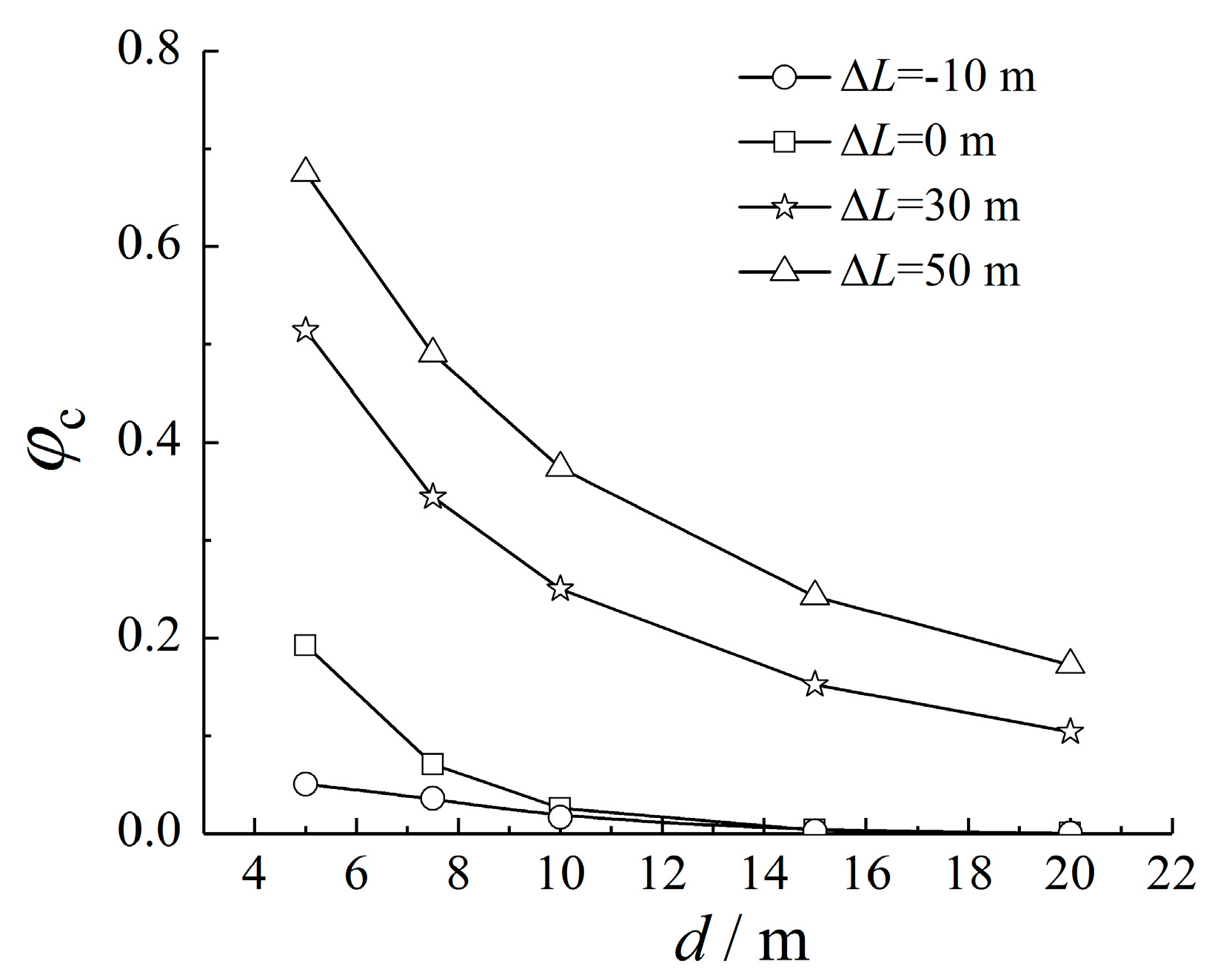
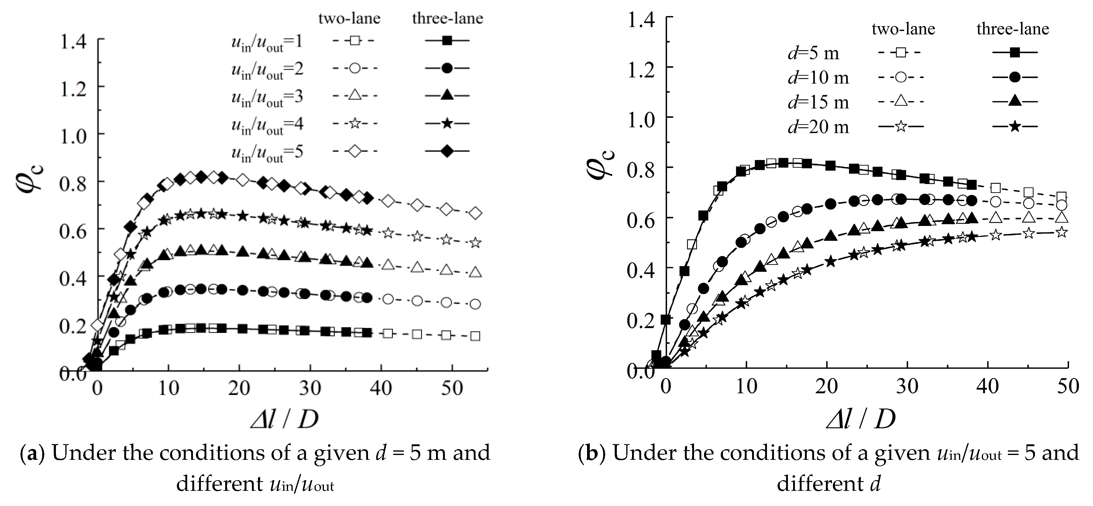
3.2.2. The Relationship between Circulating Air Mixing Ratio and Tunnel Structure Parameters

Figure 12 shows the change rule of circulating air mixing ratio φ_c with lateral distance d. With the increase of d, φ_c under each type of staggered distance ∆l decreased nearly exponentially. The smaller the ∆l is, the smaller the φ_c will be. For example, when d = 10 m, φ_c falls below 3% under the conditions of ∆l = 0 m and ∆l = −10 m, while φ_c is still up to 25.0% and 37.4% under the conditions of ∆l = 30 m and ∆l = 50 m, respectively.

Figure 13 shows the change rule of φ_c with ∆l/D for a two-lane tunnel and a three-lane tunnel. It can be observed that there is no direct relationship between φ_c and the tunnel portal hydraulic diameter D, but φ_c varies with the increase of ∆l/D.

When ∆l ≤ 0, the bigger the ∆l is, the more intense the impacts of the negative-pressure zone at the tunnel inlet on the jet flow at the tunnel outlet will be and the faster the u_max will be attenuated (Figure 8a). Therefore, φ_c rises with the increase of ∆l/D. Take the curve d = 5 m in Figure 13b as an example. At ∆l/D = −1.2, the inlet is placed behind the outlet, and combined with Figure 9a, it can be found that the influence of the negative-pressure zone at the inlet on the jet structure at the outlet is very limited, and the jet flow fully develops. At this time, a negligible amount of polluted air permeates into the inlet and φ_c is only 5.1%. With the increase of ∆l/D, the influence of the negative-pressure zone at the inlet on the jet structure at the outlet is gradually enhanced and φ_c increases linearly. When ∆l/D = 0, the outlet and the inlet are aligned and the negative-pressure zone at the inlet causes obvious damage to the jet structure at the outlet, but the jet flow still develops to some extent. At this instant, the polluted air partially permeates into the inlet and the φ_c is 19.3%.

When ∆l > 0, the decay rate of u_max increases firstly with increasing ∆l before witnessing a decrease afterwards (Figure 8b). So φ_c also rises firstly and then declines with increasing ∆l/D. When d = 5 m, φ_c will reach the maximum at ∆l/D = 14.6, and the bigger u_in/u_out is, the greater the variation of φ_c and φ_c at unit ∆l/D will be, as shown in Figure 13a. With the gradual increase of d, ∆l/D also rises gradually when φ_c reaches the maximum. For example, when d = 10 m, φ_c will be the maximum at ∆l/D = 26.3, as shown in Figure 13b.

3.3. Construction and Validation of Circulating Air Mixing Ratio Model

It can be learned from the analysis above that: (1) φ_c has no direct relation with the air velocity value but is related to the ratio of air velocity at the inlet and the outlet—u_in/u_out; (2) with the increase of d, φ_c decreases nearly exponentially; (3) when ∆l ≤ 0, φ_c increases linearly with the increase of ∆l/D; when ∆l>0, however, φ_c will first increase and then decrease with the increase of ∆l/D; the bigger the d is, the bigger the ∆l/D will be when φ_c is the maximum. Therefore, the functional relationship between φ_c and u_in/u_out, d, ∆l, and D can be described in the following forms:

$${\phi }_c=f\left(u_{\mathrm{in}}/u_{\mathrm{out}},d,\Delta l/dD\right)$$

(4)

Based on the CFD simulation results, setting ∆l = 0 as the demarcation point, the fitted piecewise expressions of φ_c can be obtained as follows via the software Matlab with the gradient descent method:

$${\phi }_c=\{\begin{array}{c}0.27{\mathrm{e}}^{-0.4d}{\left(\frac{u_{\mathrm{in}}}{u_{\mathrm{out}}}\right)}^{1.87}\left(0.82\Delta l/Dd+0.26\right),\Delta l\le 0\\ {\mathrm{e}}^{-2.06d^{0.11}}{\left(\frac{u_{\mathrm{in}}}{u_{\mathrm{out}}}\right)}^{0.94}\left(2.36{\mathrm{e}}^{-0.03\Delta l/Dd}-2.44{\mathrm{e}}^{-1.29\Delta l/Dd}\right),\Delta l>0\end{array}$$

(5)

A comparison between calculated results of Equation (5) and simulated values of φ_c is given in Figure 14. The goodness of fit R_new is 0.99.

The circulating air mixing ratio model (Equation (5)) was validated by the measured data of two actual tunnels with small spacing. Both of these tunnels are one-way and double-lane tunnels with a horseshoe-shaped cross section. The structural parameters of the two tunnels are shown in

Table 1. Structural parameters of the tunnels.

No.	Length L/m	Cross-Sectional Area A/m2	D/m	d/m	Δl/m	Front Slope of Tunnel Portal/°
#1	3875	54.3	7.6	8	43	15°
#2	3580	67.3	8.4	6	0	20°

.

The field measurement was conducted on a windless day. Because of the toxicity of CO, this test replaced CO with CO₂, which is less harmful, cheaper, and easier to obtain and measure. The pollutant-releasing device of the model test mainly included a CO₂ cylinder, a CO₂ two-stage pressure-reducing valve (better pressure stabilizing effect), and a vortex flow meter. In the experiment, CO₂ gas was released at about 100 m away from the outlet into the outflow tunnel so as to ensure that CO₂ was well mixed at the outlet section. The locations of measuring points in #1 tunnel are shown in Figure 15.

The jet velocity of the jet fan was regulated in the tunnel in order to change inlet and outlet air velocity. The air velocity of the inlet and outlet tunnel was obtained by a Testo425 thermal anemometer (Testo AG, Lenzkirch, Germany). In fact, the air velocity of a single point on the cross section of the tunnel cannot represent the average air velocity of the entire cross section. Thus, several air velocity measuring points were set on the cross section according to fluid’s characteristics of velocity distribution on the cross section of the tunnel, with the distribution of the serial numbers and the effective areas being shown in Figure 16a. Therefore, the weighted average value of the effective areas covered by the air velocities at the measuring points was the average air velocity u of the cross section of the tunnel. In other words, $u=\frac{\mathsf{\Sigma }{V}_j\Delta F_j}{\mathsf{\Sigma }F}$, where ΔF_j and V_j are the area of each part and the air velocity of the measuring point within each area. Obtaining the CO₂ concentration of the inlet and outlet tunnel by using CO₂ concentration transmitters, the arrangements of concentration measurement points are shown in the Figure 16b. As for #1 tunnel, H = 1.5 m, X = 7.0 m; as for #2 tunnel, H =1.8 m, X = 5.5 m. The arithmetic mean value of the CO₂ concentrations at these measuring points is the average concentration of the cross section of the tunnel.

Based on the measured air velocity and CO₂ concentration, φ_c can be calculated according to the following formula:

$${\phi }_c=\frac{C_{\mathrm{in}}-C_0}{C_{\mathrm{out}}-C_0}\frac{u_{\mathrm{in}}}{u_{\mathrm{out}}}$$

(6)

In the formula, C_in and C_out is the CO₂ concentration of the cross section of the inlet and outlet tunnels, respectively; C₀ refers to the local concentration of CO₂.

Meanwhile, φ_c under different u_in/u_out were predicted according to the relation model established in this paper as well as the model proposed by Tan [13]. The prediction and test results are shown in Figure 17. It shows that, calculated by measured data, φ_c gradually increases with the increasing of u_in/u_out. The variation tendency of the φ_c value predicted by Tan’s formula agrees with the measurement; however, the predicted φ_c value of #1 twin tunnels with staggered inlet and outlet is generally smaller than the measured value, and the predicted φ_c value of #2 twin tunnels with aligned inlet and outlet air tunnel portals is generally bigger than the measured value. Hence, it can be concluded that Tan’s formula is only applicable to tunnels the entrance slope gradient of which is 90° and have aligned inlet and outlet air tunnel portals, not to tunnels with staggered inlet and outlet or with relatively small entrance slope gradients. Unlike Tan’s formula, the φ_c value of #1 twin tunnels with staggered inlet and outlet predicted by the model built in this paper agrees with the variance tendency of the measured value, showing a good numerical match, while the maximum relative error is only 7.2%. Compared with Tan’s formula, the φ_c value of #2 twin tunnels with staggered inlet and outlet predicted by this model is closer to the actual measurement.

4. Conclusions

(1) For closely spaced twin tunnels with staggered inlet and outlet, the air flow discharged from their air-exhausting tunnels would diffuse transversely toward the air-inlet tunnels under the influence of the negative-pressure zone at the inlet, even causing inverse flow and forming circulating air. Parameters including inlet air velocity u_in, outlet air velocity u_out, lateral distance of the tunnel portals d, and staggered distance ∆l were all important factors influencing the circulating air.

(2) Both reducing inlet air velocity u_in and increasing outlet air velocity u_out and lateral distance d can reduce the impact of the negative-pressure zone at the tunnel entrance on the jet flow structure at the tunnel exit, thus weakening the circulating air.

(3) When the inlet is placed behind or aligned with the outlet (staggered distance ∆l ≤ 0), under the influence of the negative-pressure zone at the inlet, the jet flow at the outlet deflects entirely. The shorter the longitudinal distance between the inlet and the outlet (the larger the ∆l), the more the jet flow deflects; the quicker the jet flow maximum velocity u_max in the symmetry plane decreases, the higher the circulating air mixing ratio grows.

(4) When the inlet is before the outlet (∆l > 0), the inlet’s negative-pressure zone hardly influences the decreasing law of maximum velocity u_max in the symmetry plane of jet flow between the inlet and the outlet but changes the decreasing law of the jet flow’s u_max in other zones. With the increase of longitudinal distance between the inlet and the outlet (increase of ∆l), the decreasing velocity of u_max manifests a law that is at first increasing and then decreasing. Thus, the circulating air mixing ratio also increases first and then decreases.

(5) The quantitative relation formula of the circulating air mixing ratio for small-spaced twin tunnels with staggered inlet and outlet with air velocity ratio u_in/u_out, lateral distance of the tunnel portals d, staggered distance ∆l, and tunnel portal hydraulic diameter D is created by sections. The predictions show a good correlation with measurements. This formula supplements the limitation of the circulating air mixing ratio prediction formula which can be applied only in tunnels with aligned inlet and outlet.

(6) According to the relation model, predictions in the present research have a good correlation with measured results for tunnels with entrance slope gradients of 15° but do not relate well with those of 20°, which indicates that the front slope gradient of the tunnel portal is also one of factors affecting the circulating air mixing ratio. More in-depth research and further discussions of this will be conducted in the future.

References

1. Du, T.; Yang, D.; Peng, S.; Xiao, Y. A method for design of smoke control of urban traffic link tunnel (UTLT) using longitudinal ventilation. Tunn. Undergr. Space Technol. 2015, 48, 35–42. [Google Scholar] [CrossRef]
2. El-Fadel, M.; Hashisho, Z. Vehicular emissions and air quality assessment in roadway tunnels: The Salim Slam tunnel. Transp. Res. Part D 2000, 5, 355–372. [Google Scholar] [CrossRef]
3. Li, Q.; Chen, C.; Deng, Y.; Li, J.; Xie, G.; Li, Y.; Hu, Q. Influence of traffic force on pollutant dispersion of CO, NO and particle matter (PM 2.5) measured in an urban tunnel in Changsha, China. Tunn. Undergr. Space Technol. 2015, 49, 400–407. [Google Scholar] [CrossRef]
4. Raaschou-nielsen, O.; Andersen, Z.J.; Jensen, S.S.; Ketzel, M.; Sorensen, M.; Hansen, J.; Loft, S.; Tjonne, A.; Overvad, K. Traffic air pollution and mortality from cardiovascular disease and all causes: A Danish cohort study. Environ. Health 2012, 11, 60. [Google Scholar] [CrossRef] [PubMed]
5. Hoek, G.; Krishnan, R.M.; Beelen, R.; Peters, A.; Ostro, B.; Brunekreef, B.; Kaufman, J.D. Long-term air pollution exposure and cardio-respiratory mortality. Environ. Health 2016, 12, 43. [Google Scholar] [CrossRef] [PubMed]
6. Król, A.; Król, M. Study on hot gases flow in case of fire in a road tunnel. Energies 2018, 11, 590. [Google Scholar] [CrossRef]
7. Vega, M.G.; Diaz, K.M.A.; Oro, J.M.F.; Tajadura, R.B.T.; Morros, C.S. Numerical 3D simulation of a longitudinal ventilation system: Memorial Tunnel case. Tunn. Undergr. Space Technol. 2008, 23, 539–551. [Google Scholar] [CrossRef]
8. Maele, K.V.; Merci, B. Application of RANS and LES field simulations to predict the critical ventilation velocity in longitudinally ventilated horizontal tunnels. Fire Saf. J. 2008, 43, 598–609. [Google Scholar] [CrossRef]
9. Moosavi, E.; Shirinabadi, R.; Rahimi, E.; Gholinejad, M. Numerical modeling of ground movement due to twin tunnel structure of esfahan subway. Iran. J. Min. Sci. 2018, 53, 663–675. [Google Scholar] [CrossRef]
10. Wu, C.S.; Li, J.X.; Chen, X.; Xu, Z.P. Blasting in twin tunnels with small spacing and its vibration control. Tunn. Undergr. Space Technol. 2004, 19, 518. [Google Scholar] [CrossRef]
11. Miao, S.J.; Fu, D.F. Case study of nanjing inner ring on air pollution dispersion from roadway tunnel portals. Adv. Mater. Res. 2013, 610–613, 1895–1900. [Google Scholar] [CrossRef]
12. Chen, W.; Guo, X.; Cao, C.; Dai, Y.; Wu, G.; Tan, X.; Yang, J.; Jia, S.; Yu, H.; Li, F. Research on interrelationship of exhaust air of highway forked tunnel and countermeasures. Chin. J. Rock Mech. Eng. 2008, 27, 1137–1147. [Google Scholar] [CrossRef]
13. Tan, X.; Chen, W.; Dai, Y.; Wua, G.; Yang, J.; Jia, S.; Yu, H.; Li, F. Experimental research on the mixture mechanism of polluted and fresh air at the portal of small-space road tunnels. Tunn. Undergr. Space Technol. 2015, 50, 118–128. [Google Scholar] [CrossRef]
14. Yang, Y.; He, C.; Zeng, Y. Numerical simulation for the pollution effect between portals of twin highway tunnels. Mod. Tunn. Technol. 2009, 46, 94–98. [Google Scholar] [CrossRef]
15. Li, H.; Wang, X.; Zhou, H.; Chang, B.; You, H. Numerical analysis and countermeasures for air cross pollution at the outlets of closely-spaced tunnels. Mod. Tunn. Technol. 2009, 46, 58–63. [Google Scholar] [CrossRef]
16. Launder, B.E.; Spalding, D.B. The numerical computation of turbulent flows. Comput. Methords Appl. Mech. Eng. 1974, 3, 269–289. [Google Scholar] [CrossRef]
17. Versteeg, H.K.; Malalasekera, W. An Introduction to Computational Fluid Dynamics: The Finite Volume Method, 2nd ed.; Pearson Education: London, UK, 2007; pp. 186–190. [Google Scholar]
18. An, X.; Song, B.; Tian, W.; Ma, C. Design and CFD simulations of a vortex-induced piezoelectric energy converter (VIPEC) for underwater environment. Energies 2018, 11, 330. [Google Scholar] [CrossRef]
19. Patankar, S.V. Numerical Heat Transfer and Fluid Flow, 1st ed.; Hemisphere Pub. Corp.: New York, NY, USA, 1980; pp. 33–35. [Google Scholar]
20. Hong, S.W.; Exadaktylos, V.; Lee, I.B.; Amon, T.; Youssef, A.; Norton, T.; Berckmans, D. Validation of an open source CFD code to simulate natural ventilation for agricultural buildings. Comput. Electron. Agric. 2017, 13, 80–91. [Google Scholar] [CrossRef]
21. Mangani, L.; Buchmayr, M.; Darwish, M. Development of a novel fully coupled solver in openfoam: Steady-state incompressible turbulent flows. Numer. Heat Transf. Part B Fundam. 2014, 66, 1–20. [Google Scholar] [CrossRef]
22. Rajaratnam, N.; Pani, B.S. Three-dimensional turbulent wall jets. J. Hydraul. Div. 1974, 100, 69–83. [Google Scholar]
23. Agelin-Chaab, M.; Tachie, M.F. Characteristics of Turbulent Three-Dimensional Wall Jets. J. Fluids Eng. 2011, 133, 21201. [Google Scholar] [CrossRef]
Figure 1. Sketch map of closely spaced twin tunnels with staggered inlet and outlet.
Applsci 08 01365 g001
Figure 2. Schematic diagram of gird.
Applsci 08 01365 g002
Figure 3. Velocity profile in different mesh resolution.
Applsci 08 01365 g003
Figure 4. The decay of maximum velocity umax in the plane of symmetry of the wall jet.
Applsci 08 01365 g004
Figure 5. Nondimensional velocity profiles in the plane of symmetry of the wall jet.
Applsci 08 01365 g005
Figure 6. Impacts of outlet air velocity uout on φc.
Applsci 08 01365 g006
Figure 7. The sketches of three-dimensional velocity profiles of jet flow at tunnel exit.
Applsci 08 01365 g007
Figure 8. The decay of nondimensional maximum velocity umax in the symmetry plane.
Applsci 08 01365 g008
Figure 9. Flow structure at the portals of twin tunnels with small spacing.
Applsci 08 01365 g009
Figure 10. Impacts of air velocity u on circulating air mixing ratio φc.
Applsci 08 01365 g010
Figure 11. Impacts of velocity ratio uin/uout on circulating air mixing ratio φc.
Applsci 08 01365 g011
Figure 12. Impacts of lateral distance d on circulating air mixing ratio φc.
Applsci 08 01365 g012
Figure 13. Impacts of ∆l/D on circulating air mixing ratio φc.
Applsci 08 01365 g013
Figure 14. Comparison of calculated circulating air mixing ratio φc with simulated results.
Applsci 08 01365 g014
Figure 15. The locations of measuring points.
Applsci 08 01365 g015
Figure 16. Distribution of velocity measuring points.
Applsci 08 01365 g016
Figure 17. Comparison of predicted circulating air mixing ratio φc with measured results.
Applsci 08 01365 g017