A Study on Optimal Compensation Design for Meteorological Satellites in the Presence of Periodic Disturbance

Featured Application

This work may be used to improve the accuracy of attitude stability of flexible meteorological satellites.

Abstract

Periodic disturbance may cause serious effects on the attitude of meteorological satellites, and the attenuation of periodic disturbance is required. In this paper, a fundamental study on the optimal design of constant compensations against known-law periodic disturbance for meteorological satellites is investigated. An analytical solution for the relationship between the frequency and amplitude ratios and the response of a typical second-order vibration system is firstly derived. The compensation and disturbance torques are determined according to practical engineering. The criteria for designing the optimal compensations are based on the analytical and simulation results. Then, the criteria are applied to a flexible spacecraft actuated by constant control torque in the presence of sustained periodic disturbance. The optimal compensation torque parameters for spacecraft are acquired based on former criteria. The compensate effectiveness of the optimal compensation torque is provided and compared with results of other selections in the frequency and amplitude ratio domain. Numerical simulation results and experimental results clearly demonstrate the good performance of proposed criteria. This work provides a significant reference for the vibration attenuation of meteorological satellites in the present of periodic disturbance.

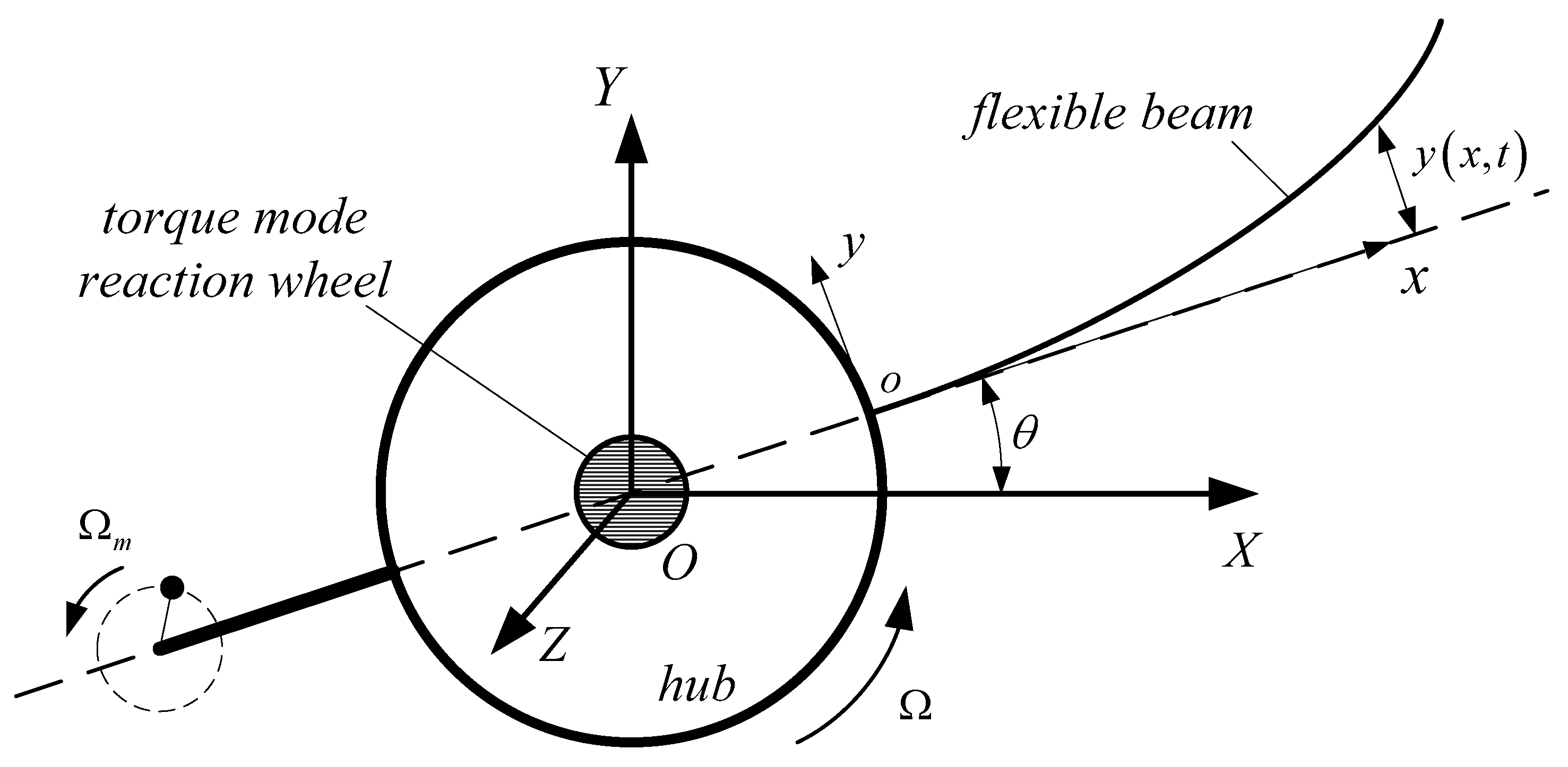
1. Introduction

Meteorological satellites play a vital role in our daily life. To send back high-quality images, satellites have to meet stringent demands related to attitude accuracy [1,2,3]. However, periodic disturbances from spaceborne equipment result in difficulty in retaining stability in the attitude of spacecraft. The application of spaceborne microwave imaging instruments has substantially improved the image definition, but poor effects on attitude accuracy are also brought about by their known-law rotating imbalance [4,5,6]. Furthermore, characteristics like flexibility and low weight make spacecraft vulnerable to vibrations caused by numerous sources [7]. In this paper, we focus on the compensation of known-law long-lasting periodic disturbances and attenuation of vibrations to improve the attitude accuracy of meteorological satellites.

Many studies have been done on the attitude control of meteorological satellites. Mitigation of the periodic disturbances by compensating torques has been proposed by researchers over the course of the past years. Zhang et al. [8] presented a fault tolerant control for external disturbances and actuator failures. This controller is the combination and application of the free weighting matrices method and LMI (linear matrix inequality) technique. However, this simply designed controller has not been well verified for flexible spacecraft. Cong et al. [9] presented an improved sliding mode attitude control algorithm with an exponential time-varying sliding surface. This controller enhanced the accuracy of maneuver in the presence of disturbances and parametric uncertainties. To reduce the dependence of estimate accuracy on a disturbance model, Hu et al. [10] designed a sliding mode disturbance observer for the attitude control of a rigid spacecraft in the presence of disturbance and actuator saturation. The adaptive controller has also been adopted. Unfortunately, the studies neglected the flexibility of the structure. The attitude control and disturbance rejection have been studied for flexible spacecraft during attitude maneuvering by Zhong et al. [11]. An improved compensator is developed to achieve asymptotic disturbance rejection. Then, a new robust state feedback controller is presented for the attitude maneuver. The proposed strategy achieved the maneuver process in the presence of small amplitude disturbances. Zhang et al. [12] proposed a generalized-disturbance rejection (GDR) control for vibration suppression of flexible structures in the presence of unknown continuous disturbances. The unknown disturbances are estimated by a generalized-disturbance rejection which is defined by a refined state space model. Chen et al. [13] focused on the disturbance observer-based control method to attenuate or reject disturbances for a spacecraft attitude control system. The disturbance observer is used to estimate the disturbances. Also, the feedforward compensation is given according to the corresponding results. Ma et al. [14] developed an adaptive failure compensation approach for the attitude control of satellites in the presence of disturbance and uncertain failures of actuators. This research mainly focuses on the disturbances from actuator failures; external disturbances have not been sufficiently considered. Lau et al. [15] improved the research on disturbance identification and rejection. The dipole-type disturbance rejection filter is adopted and applied in [15]. Subsequently, two simple close-loop system identification methods are introduced to improve the robustness of the rejection filter relative to frequency uncertainty. Chen et al. [16] made contributions to the rejection of general multi-periodic disturbances. The multi-periodic disturbances are estimated by a new presented method. Based on the estimation results, a new adaptive control method is applied for disturbance rejection. The residual vibration can be controlled in a specified range under the provided strategy. However, this approach assumes that all periods of disturbances should be known, which is difficult in practical engineering. Although the preceding strategies have made some achievements in disturbance rejection, parameter magnitudes considered in research, like the variation range of disturbance frequency and disturbance amplitudes, are not large enough. Furthermore, corresponding experiments verifying their effectiveness are absent in most literature, and it is unpractical to output complicated desired compensating torques by any actuators.

Maneuver actuators may also affect the attitude accuracy. Speaking of the actuators, jet thrusters are inappropriate for persistent disturbance. Reaction wheels are extensively used due to their advantage in generating continuous and precise torques without expending the propellant [17,18]. Although it is easy for torque mode reaction wheels to output a constant value torque, evident faults exist when tracking an expected time varying torque [19]. Most of the present papers failed to consider the capability of reaction wheels. These complex control output torques may be unfulfillable in common practical engineering. On the other hand, problems like time delay may be solved by the using of flywheel actuators. Sabatini et al. [20,21] tackled the problem of controlling time delayed systems. A prediction of state at the time of the control application has been performed to compensate for the time delay. A Kalman filter and the GNC loop were used to realize this purpose. Sabatini et al. also conducted research to test and improve the robustness of presented algorithm. Simulations and experiments were provided to confirm the effectiveness. Those works may cover the shortage caused by the time delay. Further, for meteorological satellites in the presence of known laws of periodic disturbances, those methods are inappropriate and superfluous. Based on those facts, for the compensation of periodic disturbed torques, constant reaction wheel torques may be the most practical and appropriate way. Unfortunately, work is limited on this issue in the literature.

Another way to improve the attitude accuracy of meteorological satellites is to actively suppress the residual vibrations of flexible appendages. This kind of strategy has been widely used in the attitude maneuver of spacecraft. Numerous studies have been presented for vibration suppression of flexible appendages. Smart materials, such as Magnetorheological Material (MR) [22], Piezoelectric Material (PM) [23,24], have been investigated and fabricated to eliminate the residual vibrations during the past decades. A wide range of control schemes has been proposed for the use of smart materials, such as positive position feedback (PPF) control [25], sliding mode control (SMC) [26], H-infinity control [27], and so on. However, these actuators and sensors have changed the structural property by mechanical interference, which is undesirable in many practical engineering applications. An active vibration suppression method called component synthesis vibration suppression (CSVS) can suppress vibration without additional structures attached to flexible structures. This method was first proposed by Liu et al. [28]. Then, Hu et al. [29] extended the application of the CSVS method in the attitude maneuver of spacecraft. However, as a feedforward control scheme, the application of the CSVS method is limited to the sensitivity to parameter uncertainties. Similar to the CSVS method, the input shaping technique is also used for vibration suppression. Kong et al. [30] extended the input shaping method by combining it with feedback control for the vibration control of flexible spacecraft during attitude maneuver. Their work remedied the shortcoming of input shaping as it is a feedforward control scheme. However, this technique is suitable for zero to zero maneuver. It is not appropriate for problems forced in this paper in which the disturbance is nonstop. All those tactics mentioned above have application in vibration attenuation of flexible appendages, but their application conditions are restrictive. They are not suitable for situations in which satellites are actuated by sustained disturbances. Motivated by the preceding discussion, finding an appropriate continuous compensating torque to attenuate the vibration of flexible appendages is the optimal option. However, direct studies about relationships between selection of compensate torques and vibration attenuation effectiveness for meteorological satellites are scarce.

In this paper, based on the requirement of meteorological satellites and practical limitations, step torques given by reaction wheels are adopted to compensate for the sinusoidal periodic disturbance. Two coefficients, frequency ratio and amplitude ratio, are introduced as parameters. A typical 2-order vibration system and a flexible spacecraft system are introduced. The optimal compensate torques and corresponding effect will be discussed by analytic methods. Residual vibrations are regarded as the standard of the disturbance compensate effect. To verify the effectiveness of the proposed strategy, simulation results are presented. We aim to determine the relationship between the selection of the two ratios and disturbance compensate effectiveness. Furthermore, an experimental study is provided to verify the effectiveness of the proposed strategy. It is hoped that the work will be helpful for solving practical engineering problems. In addition, preliminary investigations in this paper have limitations, and further discussions will be summarized in our next study.

The remaining part of this paper is organized as follows. Section 2 gives the mathematical modelling. Analytical relationships between ratios and residual vibration are given in Section 3. Numerical simulations, experiment results and discussions are presented in Section 3. Section 4 concludes the paper.

2. Materials and Methods

2.1. Modelling of the Flexible Spacrcraft

Three-axis spacecrafts with flexible appendages have a complex model. It is difficult for us to obtain the relationship between vibrations and control torques. To stress the key point of this paper, here we provided a simplified spacecraft model: A flywheel actuated single-axis gas suspending rotary table (SGSRT) is applied. The diagram of the SGSRT is shown in Figure 1.

As is shown in Figure 1, this system is mainly consists of a rigid hub and a flexible beam. A rigid beam is fixed on the opposite side of flexible beam. An eccentric mass is rotating around the tip of the rigid beam at a constant angular velocity. A reaction wheel is placed at the centre of the hub. Define $OXYZ$ as the inertial frame and $oxy$ as the frame fixed on the edge of rigid hub. $\theta \left(t\right)$ is the rotation angle of the hub. $y\left(x,t\right)$ is the displacement of place $x$ in frame $oxy$. $\Omega$ and ${\Omega }_m$ are the angular velocity of rigid hub and eccentric mass, respectively. The flexible beam is assumed to be an Euler-Bernoulli beam. The Newton-Euler method is used to build the mathematical model of the system. The dynamic model of the flexible system shown in Figure 1 is

$$\{\begin{array}{c}\mathit{J}\dot{\mathit{\Omega }}+{\displaystyle \underset{0}{\overset{L}{\int }}{\mathit{r}}_{\mathit{b}}\times {\mathit{a}}_{\mathit{b}}dx}+{\mathit{r}}_{\mathit{m}}\times {\mathit{a}}_{\mathit{m}}{m}_m=\mathit{T}\\ EI\frac{{\partial }^{4}y}{\partial x^4}+\sigma \left[\frac{d^{2}y}{d{t}^2}+\left(R_{hub}+x\right)\frac{d^2\theta }{d{t}^2}\right]=0\end{array}$$

(1)

where $\mathit{J}$ is the rotational inertia matrix of the rigid hub. ${\mathit{r}}_{\mathit{b}}$ is the vector from the centre of the hub to an arbitrary mass point in the flexible beam. ${\mathit{a}}_{\mathit{b}}$ is the acceleration of mass points. ${\mathit{r}}_m$ is the vector from the centre of the hub to the eccentric mass. ${\mathit{a}}_m$ and $m_m$ are the acceleration and mass of the eccentric mass, respectively. $\mathit{T}$ is the actuator torque. $R_{hub}$ is the radius of the rigid hub. $EI$ is the flexural rigidity of the beam and $\sigma$ is the surface density

As the SGSRT is adopted in this study, Equation (1) can be simplified because it is a single-axis rotation system. The simplified model can be expressed as:

$$\{\begin{array}{c}J\ddot{\theta }+{\displaystyle \underset{l}{\int }(R_{hub}+x)\ddot{y}dm}+W_m{\mathsf{\Omega }}_m^2=T\\ EI\frac{{\partial }^{4}y}{\partial x^4}+\sigma \left[\frac{d^{2}y}{d{t}^2}+\left(R_{hub}+x\right)\frac{d^2\theta }{d{t}^2}\right]=0\end{array}$$

(2)

where $J$ is the rotation inertia of the system relative to the axis of rotation. $W_m$ represents the influence on the system caused by eccentric mass. It can be expressed as $W_m=P_m{\sigma }_m\sin \left({\omega }_{m}t\right)m_m$. $P_m$ is a constant parameter about the position of the eccentric mass. ${\sigma }_m$ is the horizontal distance from the eccentric mass to the tip of the rigid beam. $y=y\left(x,t\right)$ is the displacement of the flexible beam.

Using the assumed-mode method, the displacement of the flexible beam can be expressed as:

$$\mathit{y}=\left[D\right]\mathit{\eta }$$

(3)

where $\left[D\right]$ is a matrix consisting of modes of the flexible beam, $\mathit{\eta }$ is the modal coordinate vector. In consideration of the orthogonality of the mode. Equation (2) can be shown as:

$$\{\begin{array}{c}J\ddot{\theta }+\mathit{\delta }\ddot{\mathit{\eta }}+W_m{\mathsf{\Omega }}_m^2=T\\ {\mathit{\delta }}^{\mathit{T}}\ddot{\theta }+\ddot{\mathit{\eta }}+\mathit{C}\dot{\mathit{\eta }}+\mathit{K}\mathit{\eta }=0\end{array}$$

(4)

where $\mathit{\delta }$ is the coupling matrix of rotation and vibration. $\mathit{C}$ and $\mathit{K}$ are damping and stiffness matrices, respectively. It needs to be emphasized that the reaction wheel is assumed to be ideal equipment. That means it can generate ideal square torque. Furthermore, the influence on the system caused by eccentric mass is in sinusoidal law according to its expression. Hence, the two known-law kinds of torque will be adopted in the residual part.

2.2. Modelling of the Typical Second Order Vibration System

A typical second order vibration system is also used due to its advantage in distinct mathematical analytical solution. It can be shown as:

$$m\ddot{x}+c\dot{x}+kx=F$$

(5)

where $m$, $c$ and $k$ are the respective mass, damping and stiffness of the system. $F$ is the mechanical load.

3. Results and Discussion

3.1. Analysis and Design of Optimal Compensate Criterion

For many studies about vibration suppression of flexible spacecraft, their simplified mathematical model can be expressed as a 2-order vibration system, for example, like the model used in [7]. This means the 2-order vibration system can be used to illustrate the vibration characters of flexible spacecraft. In this section, the typical second order vibration system will be used for analysis of the effectiveness of disturbance compensation and to confirm the optimal compensate criterion. Sinusoidal disturbance and square compensation are adopted based on practical engineering. It should be noted that the frequencies of two kinds of torques are assumed to be the same.

Assume there are two periodic exciting forces, $F_1$ and $F_2$, acting on the system. Then the system shown in Equation (5) can be expressed as:

$$m\ddot{x}+c\dot{x}+kx=F_1+F_2$$

(6)

where

$$F_1=\{\begin{array}{cc}B,& \frac{2j\pi }{{\omega }_f}\le t<\frac{\left(2j+1\right)\pi }{{\omega }_f}\\ -B,& \frac{\left(2j+1\right)\pi }{{\omega }_f}\le t<\frac{2\left(j+1\right)\pi }{{\omega }_f}\end{array}, B\ge 0, j=0,1,2,\dots$$

$$F_2=-A\sin \left({\omega }_{f}t\right), A\ge 0$$

${\omega }_f$ is the natural frequency of both $F_1$ and $F_2$. $B$ and $A$ are the amplitudes of the square force and sinusoidal force, respectively. Periodic square force $F_1$ can be expressed by Fourier series as:

$$F_1=\frac{a_0}{2}+{\displaystyle \sum _{n=1}^{\infty }\left(a_n\cos n{\omega }_{f}t+b_n\sin n{\omega }_{f}t\right)}$$

(7)

where the coefficients are:

$$a_0=0, a_n=0, b_n=\{\begin{array}{cc}\frac{4B}{n\pi },& n=1,3,5,\dots \\ 0& n=2,4,6,\dots \end{array}$$

In this series, the fundamental harmonic has the maximal amplitude. Then, the right side of the equal sign in Equation (6) can be expressed as:

$$F_1+F_2=\left(\frac{4B}{\pi }-A\right)\sin {\omega }_{f}t+\frac{4B}{\pi }\left(\frac{1}{3}\sin 3{\omega }_{f}t+\frac{1}{5}\sin 5{\omega }_{f}t+\cdots \right)$$

(8)

Here, we introduce an auxiliary parameter called amplitude ratio, which can be expressed as $\beta =\frac{B}{A}$. Substitute Equation (8) into Equation (6), and replace $B$ by $\beta$, we have:

$$m\ddot{x}+c\dot{x}+kx={\displaystyle \sum _{i=1}^{\infty }{P}_i\sin \left(\left(2i-1\right){\omega }_{f}t\right)}$$

(9)

where

$$P_i=\{\begin{array}{cc}\frac{\left(4\beta -\pi \right)A}{\pi },& i=1\\ \frac{4A\beta }{\left(2i-1\right)\pi },& i=2,3,4,\dots \end{array}$$

Solving Equation (9), we obtain

$$x\left(t\right)={\displaystyle \sum _{i=1}^{\infty }\left\{\begin{array}{l}{e}^{-\zeta {\omega }_{n}t}\left(x_0\cos {\omega }_{d}t+\frac{{\dot{x}}_0+\zeta {\omega }_n{x}_0}{{\omega }_d}\sin {\omega }_{d}t\right)\\ +Q_i{e}^{-\zeta {\omega }_{n}t}\left[\sin {\phi }_i\cos {\omega }_{d}t+\frac{{\omega }_n}{{\omega }_d}\left(\zeta \sin {\phi }_i-\lambda \left(2i-1\right)\cos {\phi }_i\right)\sin {\omega }_{d}t\right]\\ +Q_i\sin \left(\left(2i-1\right){\omega }_{f}t-{\phi }_i\right)\end{array}\right\}}$$

(10)

where $x_0=x\left(0\right)$, ${\dot{x}}_0=\dot{x}\left(0\right)$ are the initial conditions. $\lambda =\frac{{\omega }_f}{{\omega }_n}$ is the frequency ratio.

$$Q_i=\frac{P_i/k}{\sqrt{{\left(1-{\left(2i-1\right)}^2{\lambda }^2\right)}^2+{\left(\left(4i-2\right)\zeta \lambda \right)}^2}}, {\phi }_i=\arctan \frac{\left(4i-2\right)\zeta \lambda }{1-{\left(2i-1\right)}^2{\lambda }^2}$$

For zero initial conditions system, the solution shown in Equation (10) can be expressed as:

$$x\left(t\right)={\displaystyle \sum _{i=1}^{\infty }\left\{\begin{array}{l}{Q}_i{e}^{-\zeta {\omega }_{n}t}\left[\sin {\phi }_i\cos {\omega }_{d}t+\frac{{\omega }_n}{{\omega }_d}\left(\zeta \sin {\phi }_i-\lambda \left(2i-1\right)\cos {\phi }_i\right)\sin {\omega }_{d}t\right]\\ +Q_i\sin \left(\left(2i-1\right){\omega }_{f}t-{\phi }_i\right)\end{array}\right\}}$$

(11)

Equation (11) is the final displacement formula. The first line of Equation (11) will be decreased because of damping, and only the second line will remain when system becomes stable. We can find the displacement is strongly associated with the frequency and amplitude ratio, and the fundamental harmonic is vital in the compensated force design. Numerical simulations were provided to provide the laws.

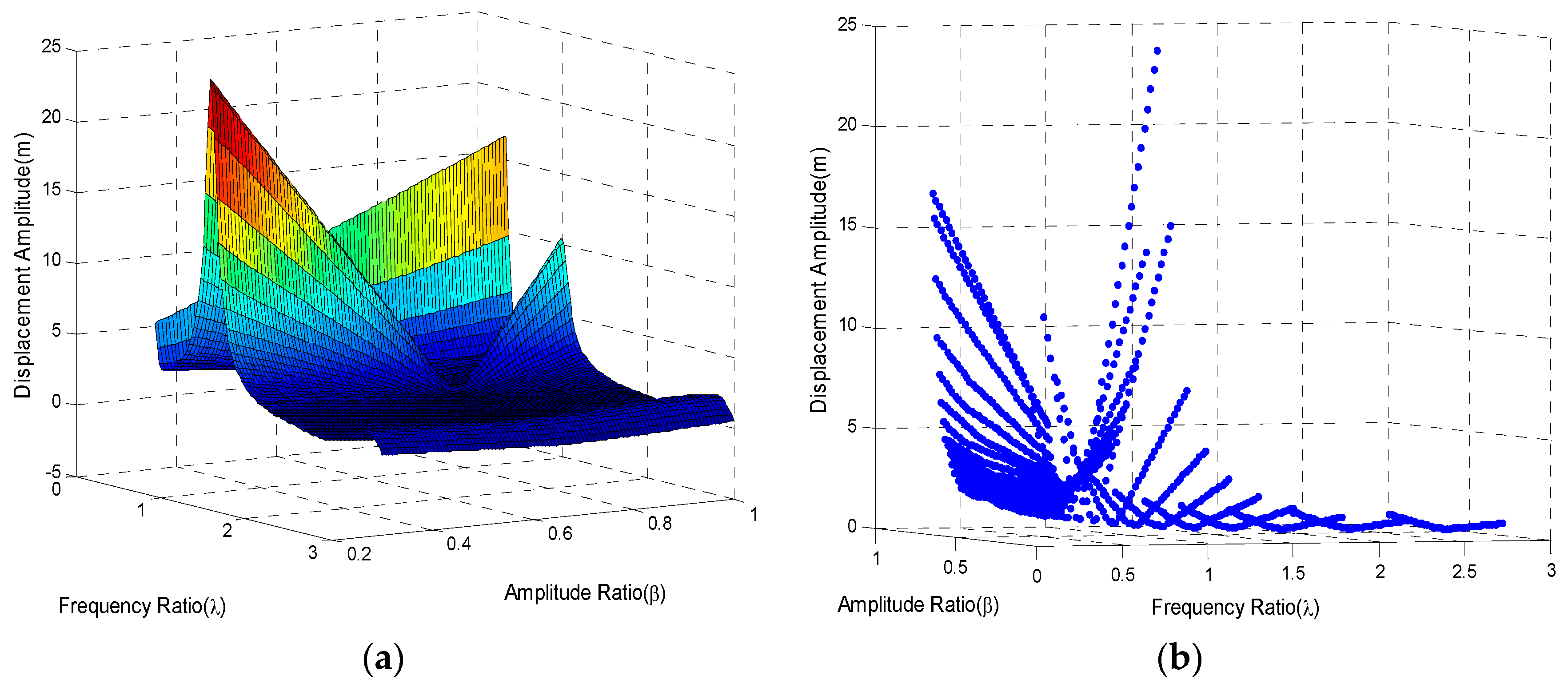
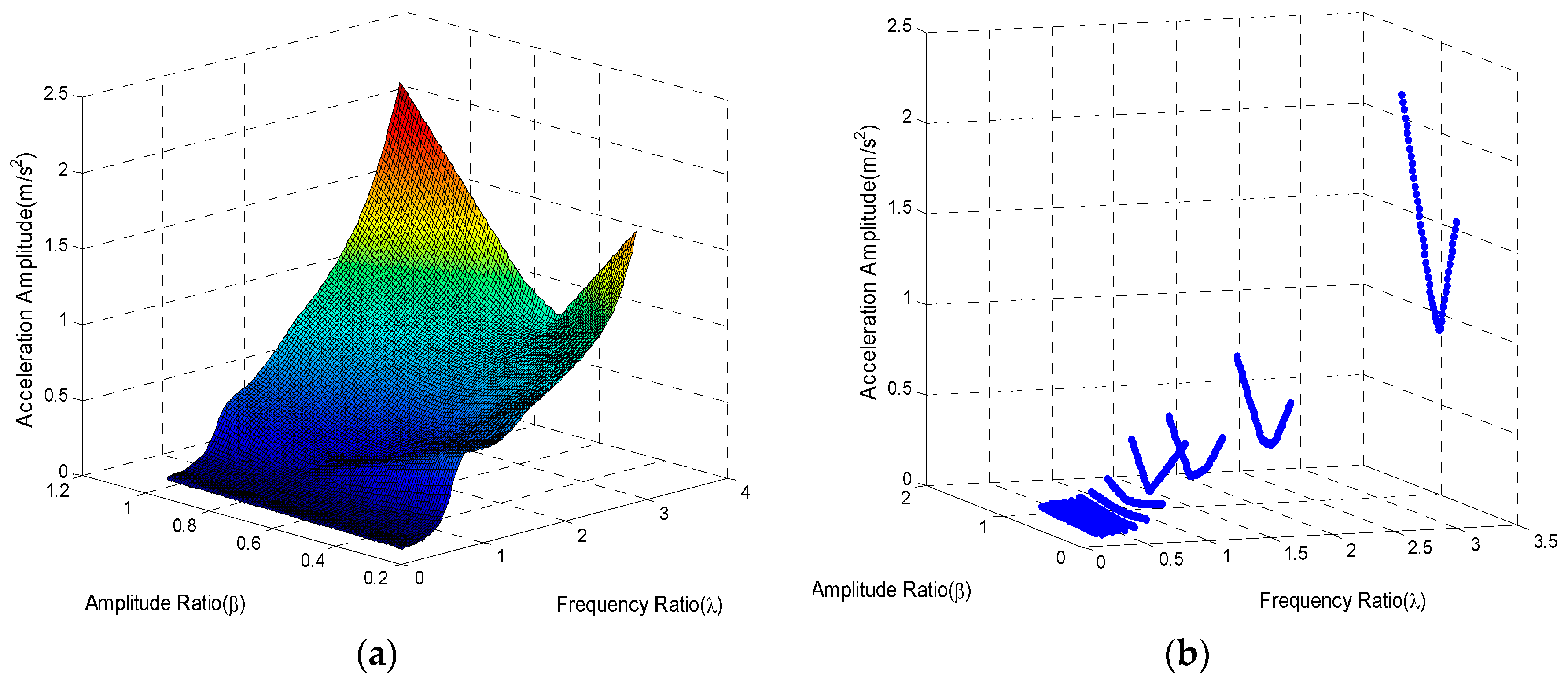
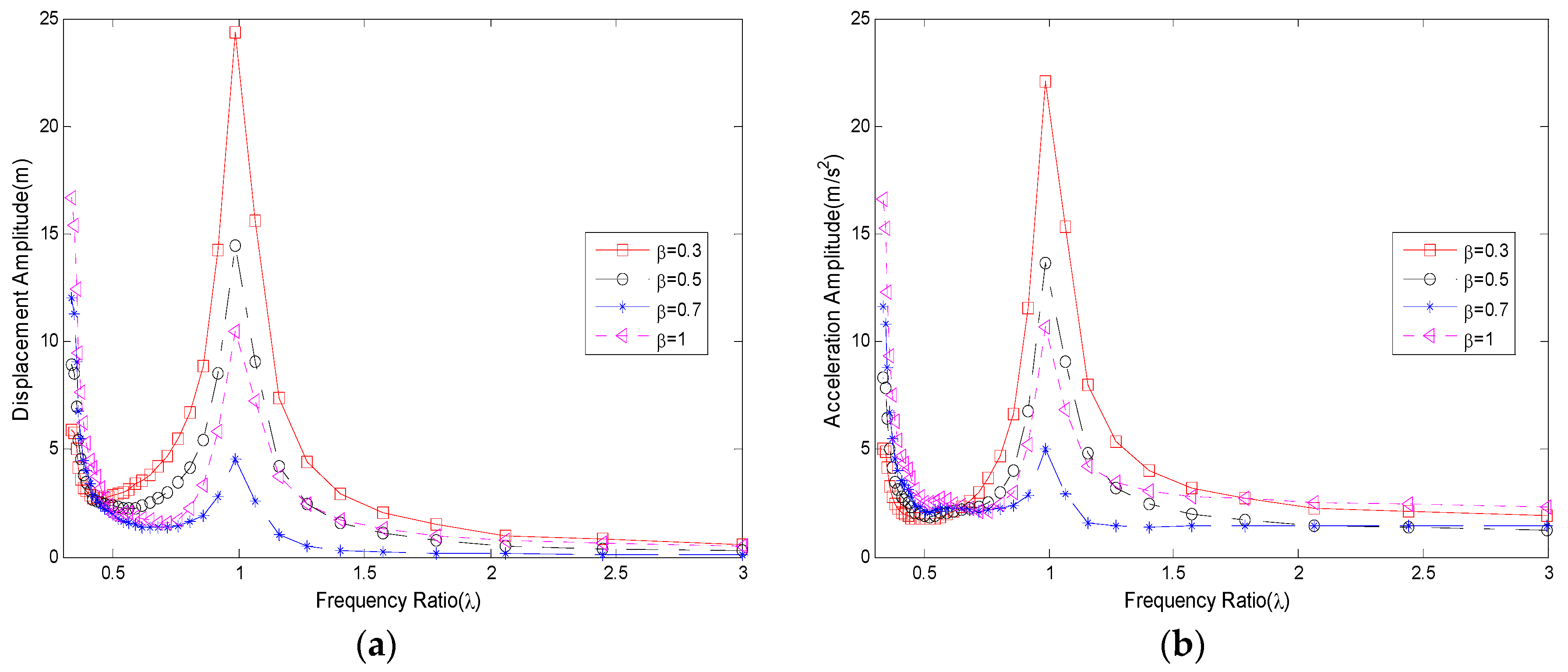
‘Simulation’ in ‘Matlab’ was used here for exact residual vibration under different combinations of the frequency ratio and amplitude ratio. For the system of Equation (6), we set its natural frequency and damping ratio as ${\omega }_{sp}=\sqrt{0.9}$ and ${\zeta }_{sp}=0.01/{\omega }_{sp}$, where the subscript ‘sp’ means mass-spring system. The amplitude value of sinusoidal disturbance $A$ is set to be 1. In this way, only amplitude ratio and frequency ratio are required. It should be noted that the parameter used here is idealized. The detailed relevance of criterion design and damping will not be considered too much here. We may study those problems in the future. The compensation effect may not notable or excessive if the two ratios are too small or too big. The range of the amplitude ratio is selected from 0.3 to 1 while the range of the frequency ratio is selected from 0.3 to 3. The tip vibration is chosen to be the standard to show the effectiveness of disturbance torque suppression. Simulation results are exhibited in Figure 2, Figure 3, Figure 4 and Figure 5.

Figure 2a,b are the total displacement results in two representations. The variation tendency is clear. At frequency ratio $\lambda =0.3$ and $\lambda =1$, residual vibrations sharply increased. These are resonances caused by different excitations. The system is mainly receiving two kinds of excitations. One is the composition of the fundamental harmonic of square force and another is the disturbance. Both of the two excitations have the same frequency ${\omega }_f$. Resonance appeared when $\lambda =1$. Another kind of excitation is the remaining harmonics of square force. Frequency of the second order harmonic almost meets the fundamental natural frequency of system when $\lambda =0.3$. As a result, resonance will appear again in the frequency ratio-domain. For each frequency ratio, there is always an amplitude ratio where the residual vibration reaches the minimum. For most frequency ratios, the best compensation effect appeared near the amplitude ratio $\beta =0.7$. The result for frequency ratio $\lambda =1$ is a typical case. For every frequency ratio, the fundamental harmonic of the square force compensates the sinusoidal force near $\beta =0.7$. Those facts illustrated that $\beta =0.7$ is the optimal option for most feasible frequency ratios.

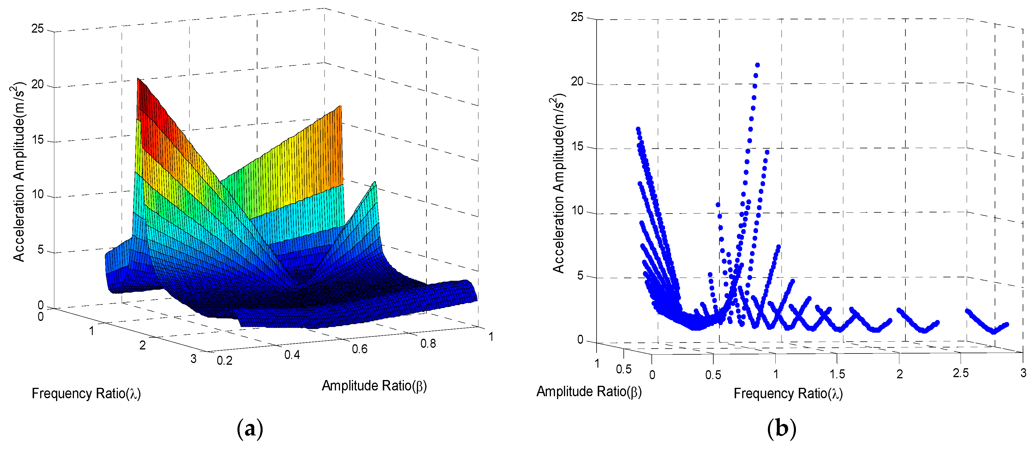
Figure 3a,b provides the accelerations with different combinations of the amplitude and frequency ratio. From the results, we can find that the variation laws are the same as those for the displacement results. Resonances are obvious at $\lambda =1$ and $\lambda =0.3$. Beyond that, values vary homogeneously at different frequency ratios. The condition under which residual vibrations always have a minimum value for each frequency ratio is also distinct, especially for frequency ratios larger than 1. The minimum values are at about the centre of the amplitude ratio range. To show the results more clearly, Figure 4 and Figure 5 show the comparisons between different ratios.

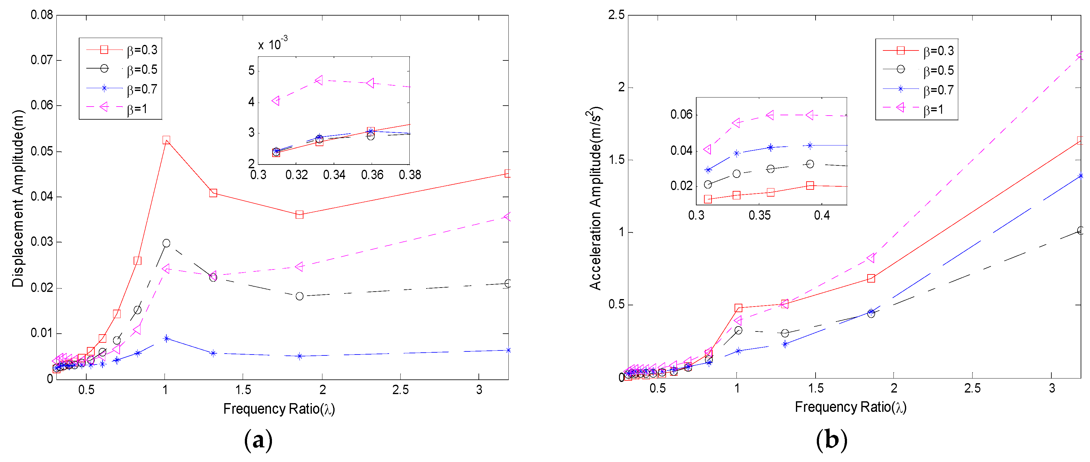
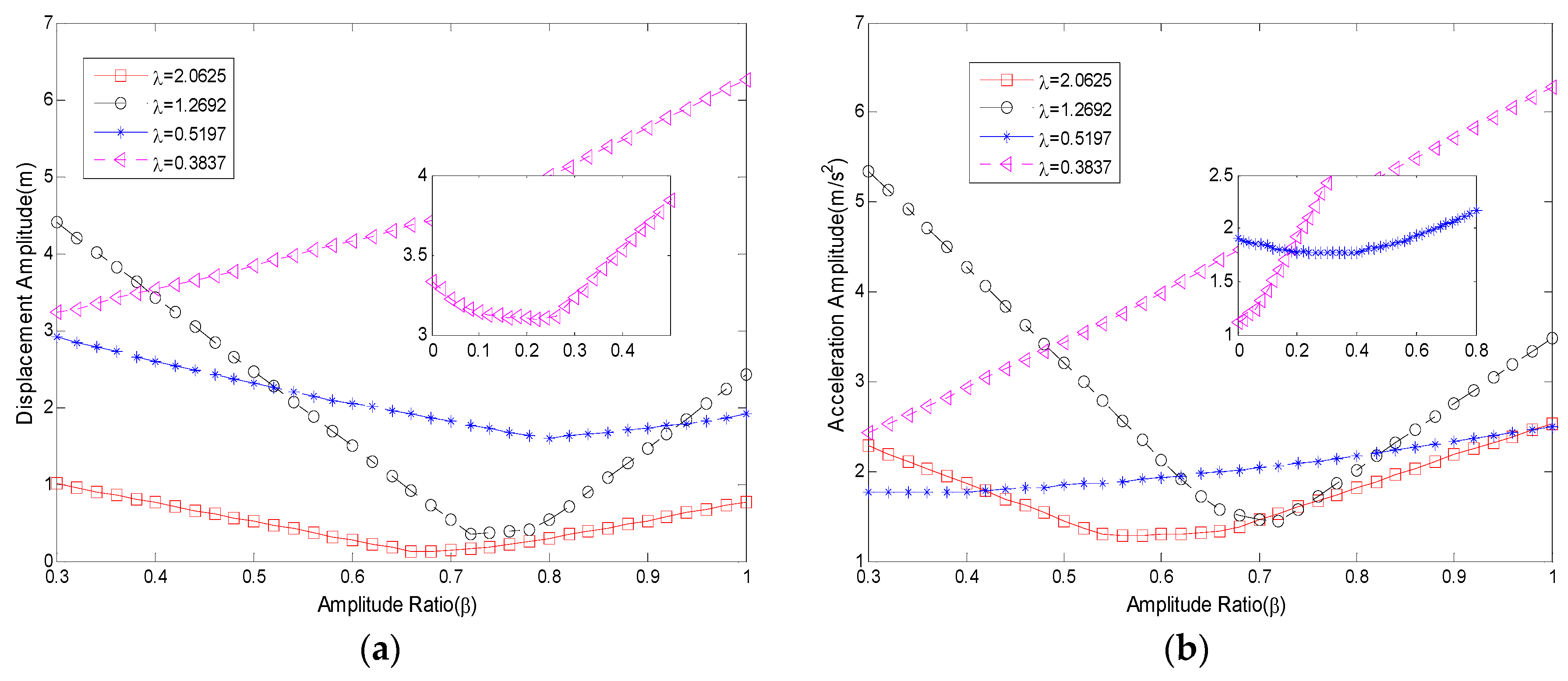
Figure 4a,b are parts of the results shown for the frequency ratio-domain. Four equally distributed amplitude ratios are selected. Data in two figures have the same variation laws. Situations when amplitude ratio $\beta =0.7$ are the best as their vibrations are the smallest for almost all the frequency ratios. That is because the sinusoidal disturbance is properly counteracted by the fundamental harmonic of the step force. Resonance is conspicuous at frequency ratio $\lambda =0.3$ and $\lambda =1$.

Figure 5a,b are parts of the results shown for the amplitude ratio-domain. Each curve has its own minimum, but not all the minimums are located near $\beta =0.7$. For frequency ratios greater than 1, the minimum appeared near $\beta =0.7$. For frequency ratios less than 1, the minimum amplitude ratios are not fixed. Floating windows in Figure 5a,b illustrate that for some frequency ratios, their minimum may appear near $\beta =0.2$. However, the corresponding frequency ratios do not frequently occur in practical engineering.

Results indicate that there is always an optimal combination of the amplitude and frequency ratio for disturbance compensation. In general, we can list the optimal compensate criterion: The optimal amplitude ratio is located within 0.6 to 0.7 for most of the frequency ratios. Besides, the frequency ratio should avoid 0.3 and 1, where it may cause resonance.

3.2. Simulations for Flexible Spacecraft

The former subsection demonstrated that the square compensation force can be used to mitigate the vibration caused by sinusoidal disturbance. To demonstrate the effectiveness of compensation in flexible spacecrafts, numerical simulations and experiments are implemented. In this subsection, the flexible spacecraft model in Equation (4) is adopted, and simulation results are presented.

The system is actuated by a sinusoidal disturbance and a square compensate torque produced by a periodic rotated eccentric mass and a reaction wheel, respectively. Residual vibrations with different combinations of frequency and amplitude ratios will be given to show the effectiveness.

Here, the torque $T$ can be expressed as:

$$T=T_1+T_2$$

(12)

where $T_1$ and $T_2$ have the same expression as $F_1$ and $F_2$ in Equation (4), respectively. $T_1$ is given by the ideal reaction wheel. $T_2$ is from the periodic eccentric mass. $T_1$ and $T_2$ can be expressed as:

$$\begin{gathered} T_1=\{\begin{array}{cc}U,& \frac{2j\pi }{{\omega }_m}\le t<\frac{\left(2j+1\right)\pi }{{\omega }_m}\\ -U,& \frac{\left(2j+1\right)\pi }{{\omega }_m}\le t<\frac{2\left(j+1\right)\pi }{{\omega }_m}\end{array}, U\ge 0, j=0,1,2,\dots \\ {T}_2=-W_m{\Omega }_m^2 \end{gathered}$$

Equation (4) can be further expressed as:

$$\{\begin{array}{c}J\ddot{\theta }+\mathit{\delta }\ddot{\mathit{\eta }}={\displaystyle \sum _{i=1}^{\infty }{P}_i\sin \left(\left(2i-1\right){\omega }_{m}t\right)}\\ {\mathit{\delta }}^{\mathit{T}}\ddot{\theta }+\ddot{\mathit{\eta }}+\mathit{C}\dot{\mathit{\eta }}+\mathit{K}\eta =0\end{array}$$

(13)

where

$$\begin{gathered} P_i=\{\begin{array}{cc}\frac{\left(4\beta -\pi \right)}{\pi }{\mathsf{\Omega }}_m^2{P}_m{\sigma }_m{m}_m,& i=1\\ \frac{4{\mathsf{\Omega }}_m^2{P}_m{\sigma }_m{m}_m\beta }{\left(2i-1\right)\pi },& i=2,3,4,\dots \end{array} \\ \beta =\frac{U}{{\mathsf{\Omega }}_m^2{P}_m{\sigma }_m{m}_m} \end{gathered}$$

Substitute the first part of Equation (13) into the second formula of Equation (13), we will have:

$$\left({\mathit{I}}_{\mathit{3}}-\frac{{\mathit{\delta }}^{\mathit{T}}\mathit{\delta }}{J}\right)\ddot{\mathit{\eta }}+\mathit{C}\dot{\mathit{\eta }}+\mathit{K}\eta =-\frac{{\mathit{\delta }}^{\mathit{T}}}{J}{\displaystyle \sum _{i=1}^{\infty }{P}_i\sin \left(\left(2i-1\right){\omega }_{m}t\right)}$$

(14)

Modal solutions are complex to be predicted analytically, not to mention the multi-dimension modal. Thus, we will directly present the simulation results. Parts of parameters are measured values of experimental equipment used in our study. Others are calculated in a mathematical way. The moment of inertia of the rigid hub is $J=15$ kg·m². The damping ratios of the vibration are ${\zeta }_1={\zeta }_2={\zeta }_3=0.05$, the natural frequencies are ${\omega }_{n1}=2.11$ rad/s, ${\omega }_{n2}=13.28$ rad/s, ${\omega }_{n3}=37.15$ rad/s. The coupling matrix is $\mathit{\delta }=\left[\begin{array}{ccc}2.65& 0.54& 0.21\end{array}\right]$ kg·m². In simulations, the mass of rotating eccentric mass is $m_m=0.4$ kg, and its eccentric radius is ${\sigma }_m=0.08$ m. The states of system are initialised to be zero.

The maximum of sinusoidal disturbance will vary in a certain range depending on each frequency ratio. Square compensation torques were assumed to be ideally outputted, which means it can perfectly fit the sinusoidal disturbance. The frequency ratio range is set from 0.3 to 3.2, and the amplitude ratio range is set from 0.3 to 1. Those settings are based on the results in the previous subsection. Amplitudes of flexible beam tip residual vibration under different combinations of frequency and amplitude ratios are calculated by ‘Simulation’ in ‘Matlab’ software. Simulation results are illustrated in Figure 6 and Figure 7.

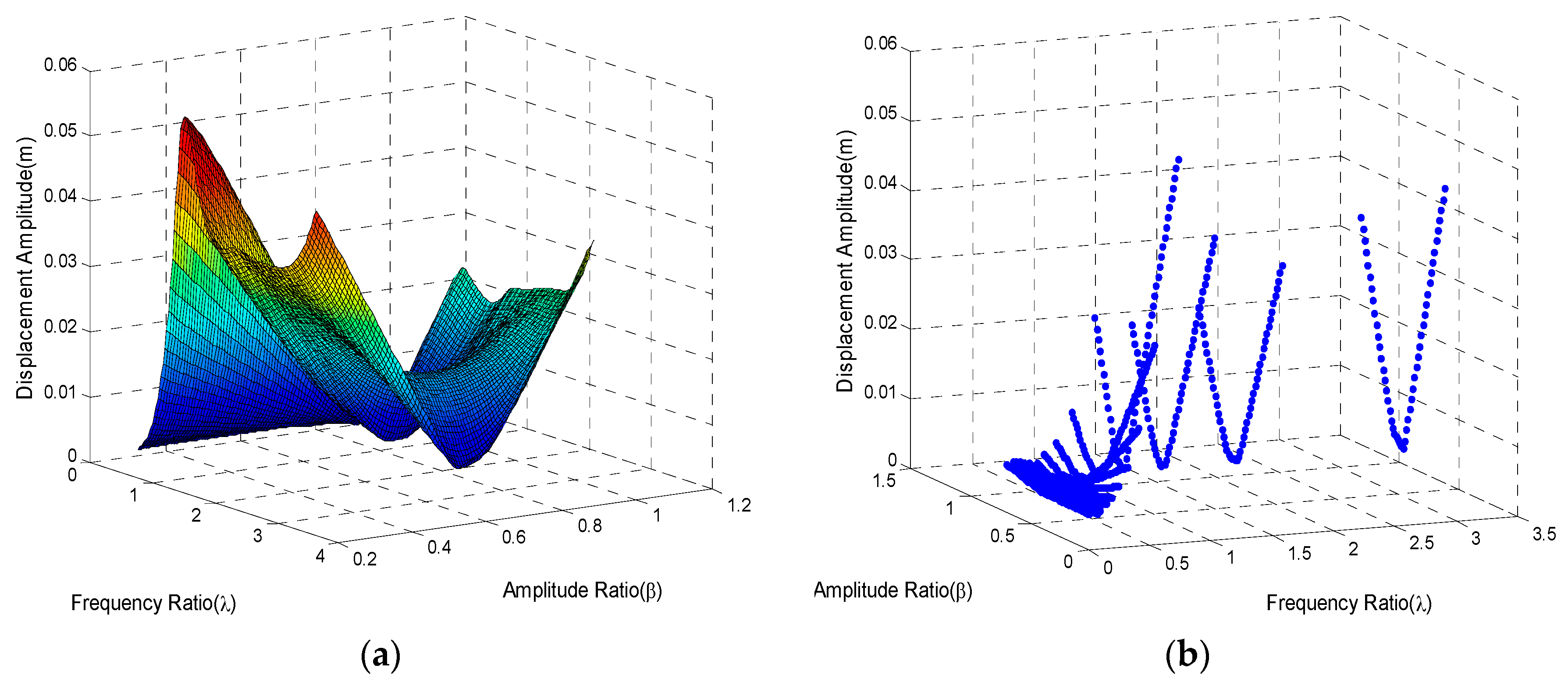
Figures 6a,b show the displacement of the flexible beam tip with all the combinations of frequency and amplitude ratio in this simulation. Similar to the results displayed in the former subsection, when the amplitude ratio is near $\beta =0.7$, the displacement of the flexible tip is minimal. This law is particularly obvious when the frequency ratio exceeds 0.5. Those results just proved the optimal criterion. Variation amplitudes are so weak that the trend is not so clear when the frequency ratio is smaller than 0.5.

Figure 7a,b are the amplitude history of the flexible beam tip acceleration. The tip acceleration is a real effect when the amplitude ratio is located near $\beta =0.7$. The frequency of the system is fixed, so the increasing frequency ratio heightened the rotation velocity of the eccentric mass, and also the amplitude of torques. As a result, values of accelerations increase with increasing frequency ratio.

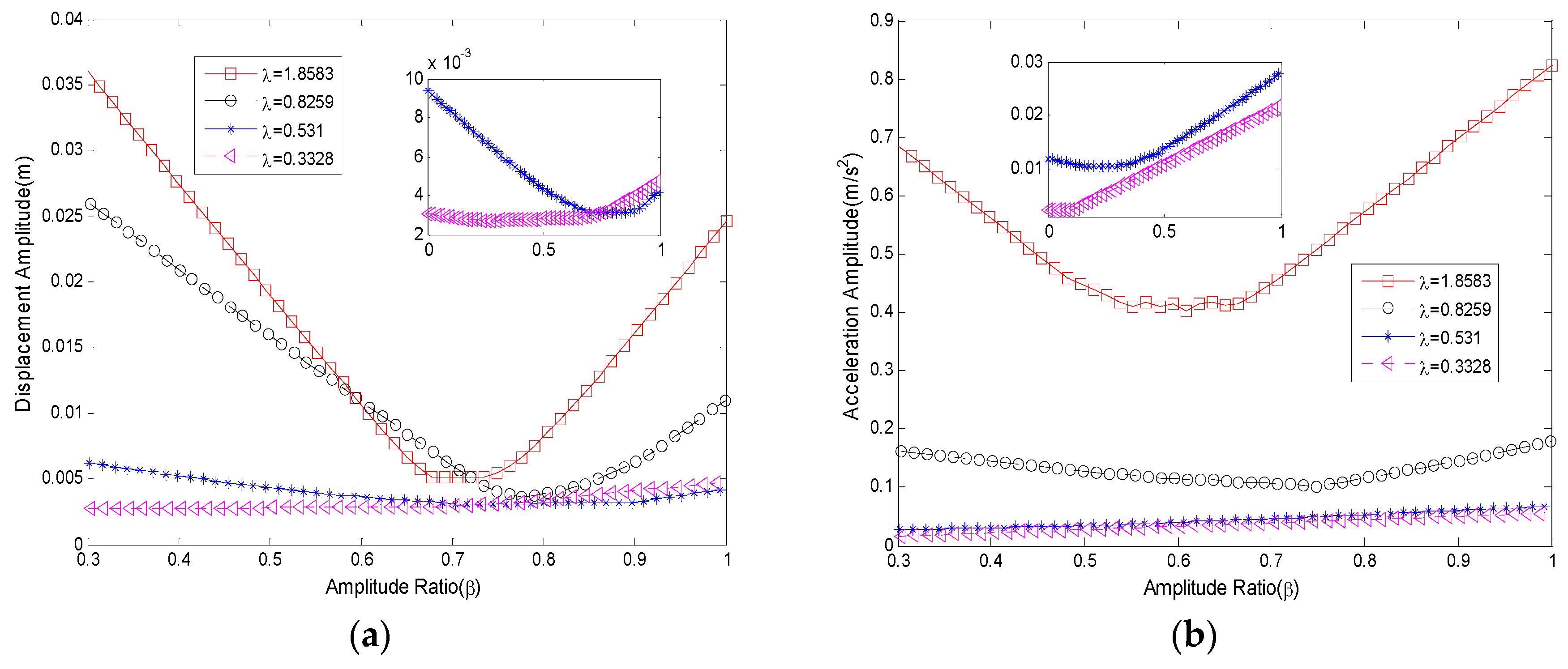
Figure 8a,b show the amplitudes of residual vibration in the frequency ratio-domain with selected amplitude ratios.

The variation tendencies in Figure 8a,b are analogous to those in Figure 4a,b. Situations with $\beta =0.7$ in the frequency ratio-domain are much smaller than those for the other three selected amplitude ratios. Resonance is obvious at $\lambda =1$ for all the amplitude ratios even though the amplitude of the synthetic torque is small. The fundamental harmonic of square torque is adopted to compensate the sinusoidal disturbance while the other orders of the harmonic become the new disturbances. Frequency of the second order harmonic meets the fundamental natural frequency of the system precisely, but amplitudes of remaining orders of the harmonic are so small to cause evident vibrations. As a result, resonances at $\lambda =0.3$, which are shown in floating windows, are not obvious. Although higher Fourier series result in new disturbances, the main effect is from the first order.

Figure 9a,b shows us how amplitudes vary in the amplitude ratio-domain under special frequency ratios.

Results revealed by Figure 9a,b demonstrated the relationship between the amplitude ratio and the level of residual vibration. The results all have the feature that the displacement amplitude always has a minimum in the amplitude ratio-domain. According to data in Figure 9a, $\beta =0.7$ is an optimal region for the compensation of disturbances. The optimal amplitude ratio for tip acceleration, shown in Figure 9b, appears to be somewhat different, but the best combination of the amplitude and frequency ratio does exist despite that the values are different for frequency ratios. All the simulation results demonstrated this for the most frequently occurring situations.

3.3. Experimental Results

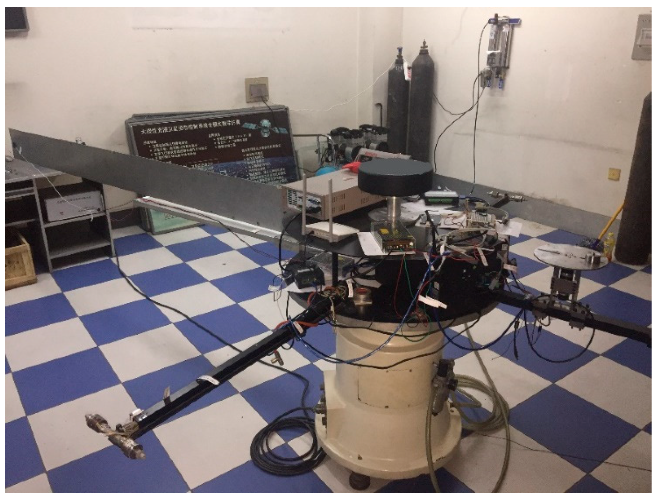
Experiments were performed on an SGSRT to verify the proposed criterion and the simulation results. The equipment is shown in Figure 10. This systems mainly consists of a single-axis rotation hub, a flexible aluminium beam ($2480\times 200\times 2.5$ mm), a torque mode reaction wheel ($T_{\max }=0.065$ Nm) whose rotation axis is coincident with the hub, a periodic rotation dish with an eccentric mass to create the disturbance, and equipment on the hub for measuring, control and data exchange.

The hub is suspended by a gas bearing. A zero-gravity environment is required, and the table is limited to rotate on the horizontal plane. The residual vibration is measured by an accelerometer fixed on the tip of a flexible beam. The model of the accelerometer ($\pm 2 g$,$0-400 Hz$) is 2220-020, produced by Silicon Designe Inc. (Kirkland, WA, USA). Eccentric mass is chosen to be 0.4 kg and 0.25 kg for different frequency ratios, and the periodic rotation dish is placed 0.6 m from the rotation axis of the system. This is the best setting to generate sinusoidal disturbance whose amplitude is within the limits of the reaction wheel.

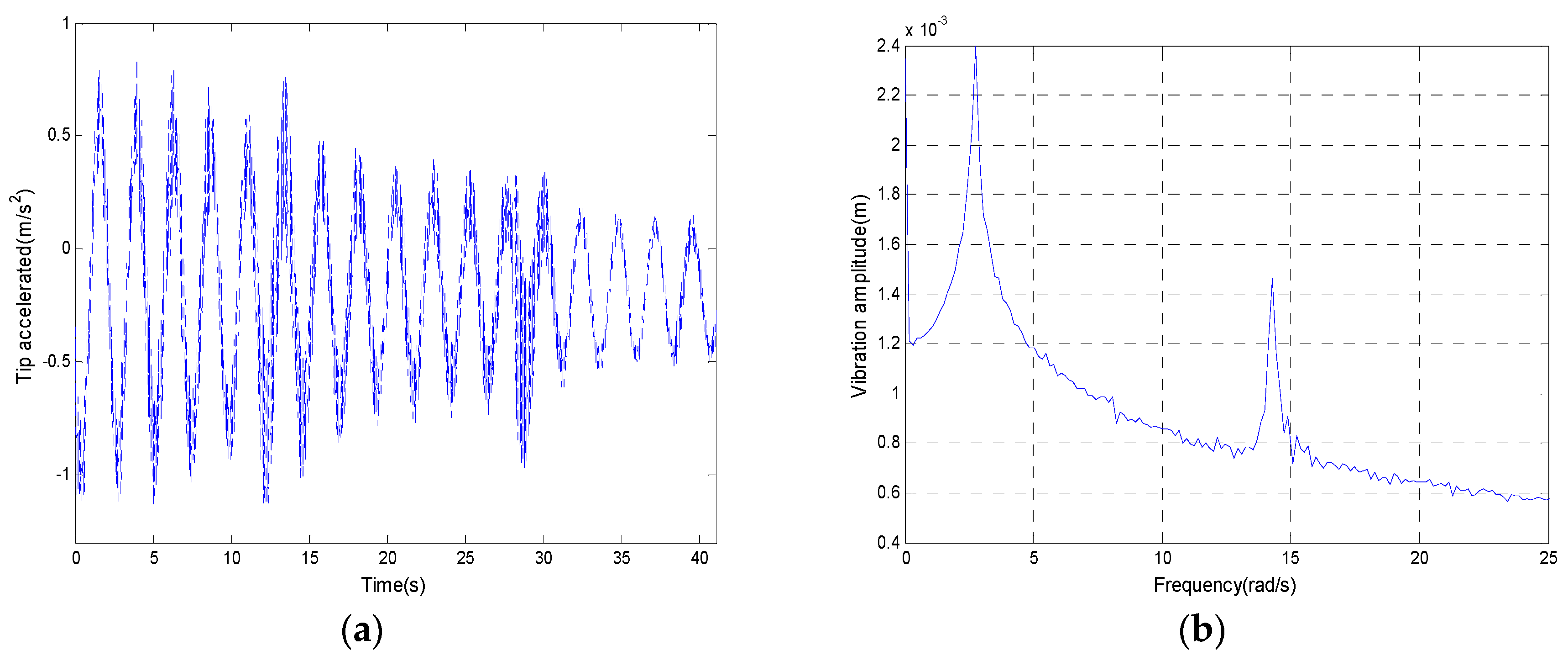
Frequencies of the experimental equipment have a close relationship with the experimental results. To identify the frequencies of the experimental equipment, free vibration tests were performed, and the fast Fourier transform (FFT) was applied. Figure 11a,b shows the measured tip acceleration data and the FFT result.

Results show that the first two vibration orders are obvious. The measured and the calculated frequencies are shown in

Table 1. The first and second frequencies (rad/s).

	1st Mode Frequency	2nd Mode Frequency
Measured	2.7382	13.9487
Calculated	2.8081	13.643
Error	2.781%	2.19%

.

The errors of the first two frequencies between measured and calculated results are 2.781% and 2.19%, respectively. In view of the difference between the experimental equipment and mathematical model, these errors are acceptable and negligible.

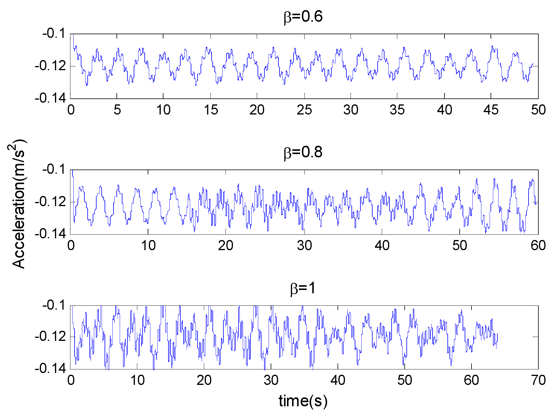
According to the previous results, there are 2 typical varying laws in the amplitude-ratio domain. For situations $\lambda <0.5$, variation is not obvious. This is because the torques are too small for flexible systems. Similarly, the torques are too large when $\lambda$ is too high. Considering those situations and the output ability of the experimental equipment, three frequency ratios 1.3, 0.9 and 0.6 were selected for the experiment. Thus, three cases of the experiment corresponding to three selected frequency ratios were provided. On the other hand, simulations illustrated that the optimal amplitude ratio for most frequency ratios is near 0.7. Thus, three amplitude ratios near 0.7 were also selected for experimental cases.

Simulations were performed with real parameters in the experiment. Zero initial conditions were provided for all the experiments. Square compensation torques from the reaction wheel and sinusoidal disturbance were started at the same time. The measured accelerations of the flexible beam tip are shown in Figure 12, Figure 13 and Figure 14.

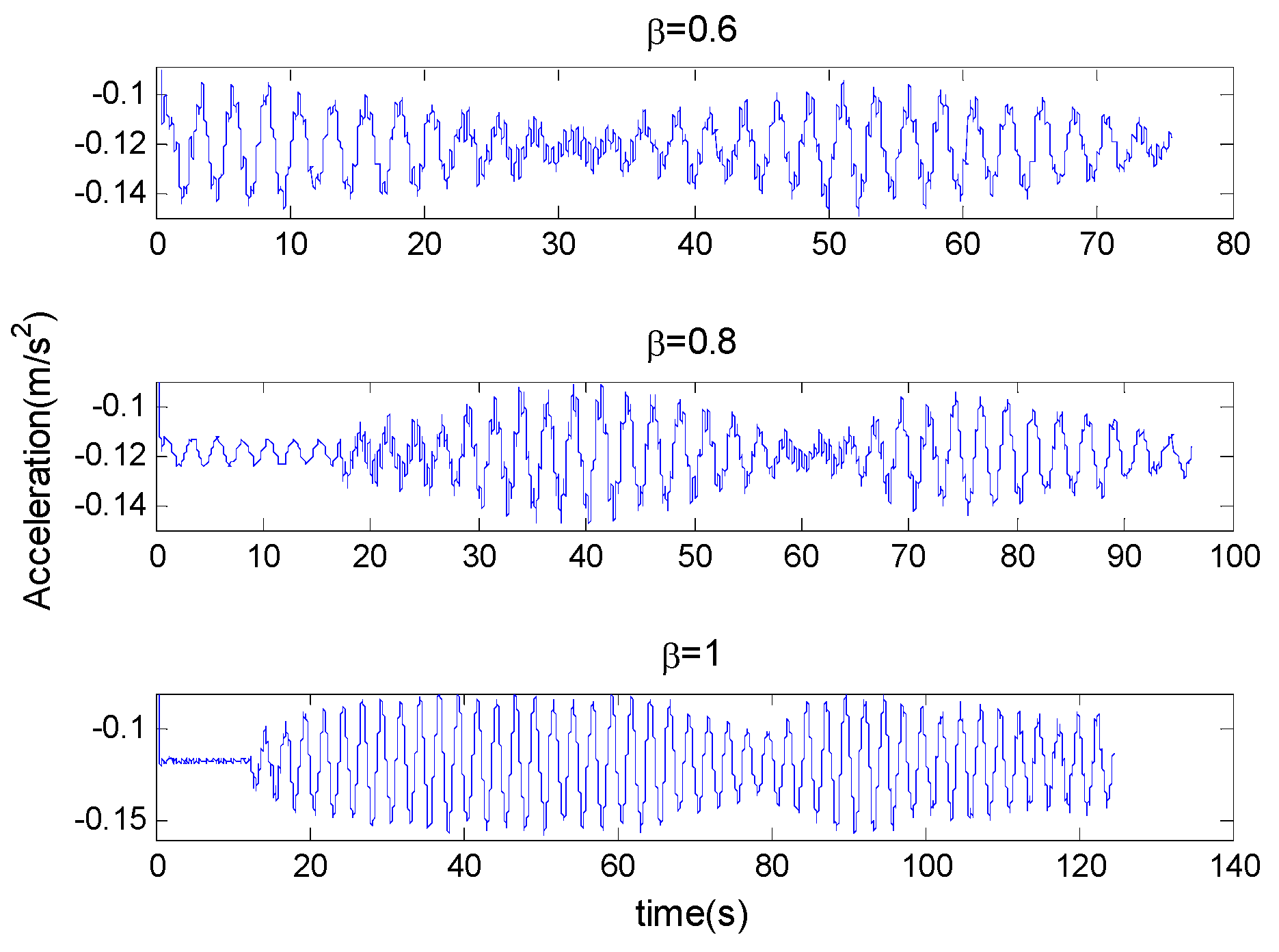
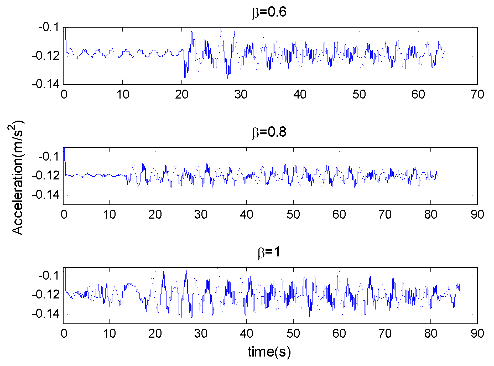
3.3.1. Case A

In this case, $\lambda =0.6$, ${\sigma }_m=0.08$ m, $m_m=0.4$ kg. Three experiments were performed with $\beta =0.6, 0.8, 1$, respectively. The tip residual accelerations are shown in Figure 12.

In case A, the frequency ratio is selected as 0.6. In this case, three typical experiments are conducted with three amplitude ratios. The measured tip accelerations are illustrated in Figure 12. The tip accelerations were recorded. It can be seen from Figure 12 that the vibration amplitude when $\beta =0.6$ is the smallest. Vibration amplitude when $\beta =0.8$ is slightly greater than that when $\beta =0.6$. However, when the amplitude ratio is 1, the residual vibrations are much more obvious than before.

3.3.2. Case B

In this case, $\lambda =0.9$, ${\sigma }_m=0.04$ m, $m_m=0.4$ kg. Three experiments were performed with $\beta =0.6, 0.8, 1$, respectively. The tip residual accelerations are shown in Figure 13.

In case B, the envelope curves are obvious. That is because the frequency of torques is close to the natural frequency of the system. As the amplitude ratio increases, the maxima of the residual vibration increase.

3.3.3. Case C

In this case, $\lambda =1.3$, ${\sigma }_m=0.04$ m, $m_m=0.25$ kg. Three experiments were performed with $\beta =0.6, 0.8, 1$, respectively. The tip residual accelerations are shown in Figure 14.

In this case, the situations when $\beta =0.6$ and $\beta =0.8$ are almost the same, but when $\beta =1$, the residual vibration amplitude increased evidently.

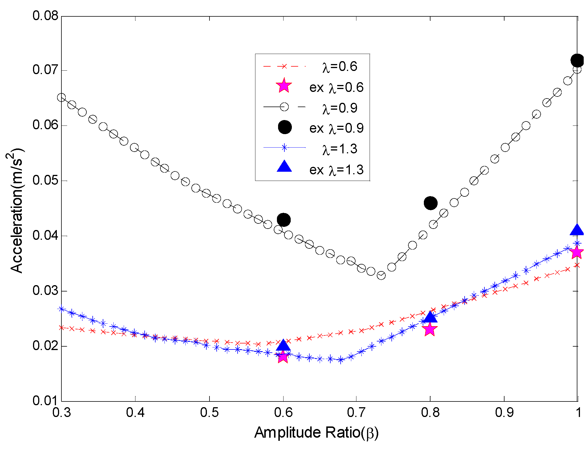
Experimental results illustrate the square torques are efficient to compensate sinusoidal disturbance, but the effects vary with different conditions. According to the results of experiments, for all the three cases, the compensation effects are almost the same when $\beta =0.6$ and $\beta =0.8$. Compared with that, situations when $\beta =1$ are worse. The amplitudes of residual vibration during compensation are listed in

Table 2. Tip acceleration amplitude with different frequency and amplitude ratios m/s².

	$\mathit{\beta }\mathbf{=}\mathbf{0.6}$	$\mathit{\beta }=0.8$	$\mathit{\beta }=1$
$\lambda =0.6$	0.020	0.025	0.041
$\lambda =0.8$	0.043	0.046	0.072
$\lambda =1.3$	0.018	0.023	0.037

.

Recall the added special simulation results which corresponded to the experiments. Figure 15 presents the results in the amplitude ratio-domain. The point marked ‘ex’ means the experimental data. The experimental results were largely in line with the simulation results. Simulation results show that the maximum amplitude of residual vibration always has a minimum point for each frequency ratio. Despite that the number of experiments is limited, the effectiveness and veracity of the proposed criterion are proved. Both experiments and simulations have verified the veracity of our study. However, it should be noted that all the experiment results are from the SGSRT, and the limitation of single axis rotation can be avoided. This limitation will be solved in future studies.

4. Conclusions

In this article, the optimal criterion of constant compensations has been investigated for flexible spacecraft in the presence of known-law sustained periodic disturbance and square torques. This criterion is mainly based on the mathematical analytical results of the typical vibration system. First, the constant square compensation torque is obtained using the Fourier expansion method, and the relationship between the response of the system and input torques is obtained. The optimal criterion is obtained according to the analysis and simulation results. The criterion exhibits advantages in a flexible spacecraft system in the presence of sustained periodic disturbance. In general, the optimal amplitude ratio is near 0.7 for most frequencies. The frequency ratio should avoid the points near 0.3 and 1. Both numerical simulations and experiments have been performed to verify the veracity of the obtained criterion. However, defects such as the disturbance being too simple and the SGSRT is equipment with only one axis rotation are obvious in our study, and extension studies will be investigated for those limitations in our future research.