Spectral Methods for Modelling of Wave Propagation in Structures in Terms of Damage Detection—A Review

Abstract

Modern methods of detection and identification of structural damage direct the activities of scientific groups towards the improvement of diagnostic methods using for example the phenomenon of mechanical wave propagation. Damage detection methods that use mechanical wave propagation in structural components are extremely effective. Many different numerical approaches are used to model this phenomenon, but, due to their universal nature, spectral methods are the most commonly used, of which there are several types. This paper reviews recent research efforts in the field to show basic differences and effectiveness of the two most common spectral methods used for modelling the wave propagation problem in terms of damage detection.

1. Introduction

Damage detection is the key aspect of Structural Health Monitoring (SHM), being defined as the acquisition, validation and analysis of technical data to facilitate life-cycle cost management decisions [1]. Numerous SHM techniques have become the subject of extensive scientific investigations [2,3]. As one of the greatest challenges of the SHM system has been recognised, the knowledge of what physical parameters observe and how to identify their ’changes’ [4]. There have been defined various techniques of efficient damage detection based on modal analysis [5,6,7,8,9,10,11], wave propagation [12,13,14,15,16,17,18,19,20,21,22,23,24,25,26,27,28,29,30], impedance changes [31,32], ultrasonic inspection [33,34,35,36,37,38], and many others [39,40,41,42,43,44].

Modern engineering is based on numerical modelling of designed structures, and it has been a standard procedure for any technical design starting from a project through a thorough state analysis until the damage prognosis operations. Almost every reliable damage detection procedure requires dynamic analyses typically distinguished according to the range of excitation frequency. It is usually categorized as structural dynamics for low frequencies (up to few hundred hertz) and wave propagation for high frequencies (the order of kilohertz) [45]. Dynamic analyses are usually performed using the conventional Finite Element Method (FEM) [46,47,48], but, for wave propagation, many higher order vibrational modes participate in the motion and the classical FEM approach may be numerically inefficient. This fact originates from the very dense FE meshes resulting from very small wavelengths participating in vibrational movements. It is known that the size of FEs should be of the size comparable to the wavelength of the shortest signal component. Therefore, numerous attempts have been addressed in order to improve other numerical methods for simulation of wave propagation in structures, especially because some important phenomena like wave dispersion or attenuation [49] should be addressed.

A process of numerical modelling of the designed structure is based on a solution of a set of partial differential or integral equations being an approximation of the problem [50,51,52,53,54,55,56,57,58,59]. There are various numerical methods to solve partial differential equations, which have been roughly gathered in

Table 1. Solution methods of numerical partial differential equations [60].

Method	Example
finite difference	e.g., parabolic, hyperbolic, finite-difference time-domain
finite volume	e.g., high-resolution
finite element	e.g., finite element, spectral element
meshless (meshfree)	e.g., material point
domain decompositions	e.g., fictitious domain
others	e.g., methods of lines, boundary element, wavelet method

.

The crucial point in the process of numerical modelling of structures is typically the balance between the time of calculation and the level of complication of the solution method chosen. As the number of SHM systems based on changes in wave propagation in structures increases every year, therefore it is important to use reliable solution methods for this type of physical phenomena [61]. For several decades, the number of applications of spectral methods for solution of wave problems has been constantly growing. According to the literature [62], the name for “spectral method” begins probably with the usage of Fourier series of sines and cosines as basis functions especially in reference to a time series evaluation and the basic frequencies of a process, i.e., the “spectrum”. However, in the most general definition, the spectral methods involve defining the solution to a problem as an abridged series of known functions of the separate variables [63]. The choice of an appropriate spectral method should be defined by the two main aspects: the accuracy and the efficiency. In order to be useful, a spectral method should be performed to provide results of greater accuracy than conventional difference methods of a similar spatial resolution. The choice of convenient spectral representation depends also on the kind of boundary conditions in the problem. The calculation results obtained by the use of spectral methods should be more accurate while compared with the results produced with conventional methods. Similarly, the efficiency of the calculation process for a comparable number of degrees of freedom should be analogous [63].

Despite the fact that there are many possibilities of computational techniques employed to solve various types of problems considered in SHM applications [61], it is very difficult to indicate one universal numerical method for such problems. Therefore, it is important to choose a method that is suitable and efficient. As presented in Table 1, there are various numerical methods of modelling of structures successfully used in [64,65,66,67,68,69,70,71,72,73,74,75,76,77,78]; however, for the problems of wave propagation modelling, the most popular are spectral methods. Two basic approaches may be distinguished. The first one has been popularised by Doyle and is named Frequency Domain Spectral Element Method (FDSEM) [79]. This method is a semi-analytical technique commonly used for modelling of guided waves propagating in 1D and 2D structural elements [26]. The governing partial differential equations (PDEs) describing the wave problem are converted into a frequency domain by the use of Fourier transform of the displacement variables. Then, it is possible to operate on a set of ordinary differential equations (ODEs) for each discretized frequency instead of on PDEs. The obtained ODEs solutions are then used as shape functions to formulate the elemental dynamic stiffness matrix. The procedure relates the transformed nodal forces to the corresponding transformed nodal displacements. Such approach, similar to the Finite Element Method (FEM), can be used to model structures with more complicated geometries. In comparison with FEM, the FDSFEM leads to significant computational efficiency, especially in modelling of anisotropic and inhomogeneous structures with damages [45]. The limitation of FDSFEM is the difficulty of mathematical modelling of finite length structures due to the problem of Fourier transform expansion into more complicated geometries. The second approach is named the Time Domain Spectral Finite Element Method (TDSFEM) and it has been found to be extremely efficient in simulating guided wave propagation in computational solid and fluid mechanics. This scheme adjusts the disadvantage of FE in terms of large computational time resulting from dense spatial and temporal discretization. The main difference between TDSFEM and FEM is the use of other types of polynomials as shape functions in the former method. The integration points in TDSFEM are usually connected with the nodes resulting in consistent diagonal mass matrix formulation helping in faster convergence [80]. TDSFEM has been successfully implemented for simulation of wave propagation in 1D, 2D and 3D waveguides [81,82,83,84], which includes modelling of piezoelectrically (PZT) induced wave propagation [83,84,85], and wave interaction with damages [86,87,88]. In many of these works, a 2D model with an appropriate plate theory has been adopted to reduce the number of degrees of freedom (DOFs) associated with 3D models [81,85,89].

As stated in [46], the spectral method [63], the spectral element method [65,90,91,92,93,94,95,96] and the spectral finite element method [45,97,98,99] and each of the following references have been developed to solve wave propagation problems. Analysing the literature resources, it is sometimes difficult to recognise whether a method belongs to one or another of these methods. However, in all cases, higher-order polynomials or harmonic functions are proposed in the solution space. There are various literature reviews regarding a comparison of different solution methods for one problem [100].

Therefore, it has been a main subject of this paper to explain the differences in the two methods most often used for modelling the problems of wave propagation. Although a variety of papers has been listed in the reference section, this survey can be incomplete and the author wishes to apologise, in advance, for any inadvertent omission of relevant publications. It was a strong intention to try to mention any important contribution to the field of wave propagation modelling by the use of two most often used spectral element methods (

Table 2. Synthetic compilation of research papers devoted to numerical modelling of different structural elements for wave propagation analysis.

Numerical Method Employed	References
FDSFEM for 1D elements	[79,101,102,103,104,105,106,107,108,109,110,111,112,113,114,115,116,117,118,119,120]
FDSFEM for 2D elements	[79,121,122,123,124,125,126,127]
TDSFEM for 1D elements	[82,128,129,130,131,132,133,134]
TDSFEM for 2D elements	[82,87,135,136,137,138,139,140,141,142,143]
TDSFEM for 3D elements	[82,85,144,145,146]

, the abbreviations used have been listed at the end of the paper).

2. Introduction to Spectral Analysis

By most general definitions, spectral methods are based on the representation of a certain function, $f\left(x\right)$, not necessarily an orthonormal set of functions, $P_n\left(x\right)$, like [62,63]:

$$f\left(x\right)=\sum _{n=0}^{\infty }{a}_n{P}_n\left(x\right),x\in [a,b],$$

(1)

with orthonormal polynomials defined as:

$$\underset{a}{\overset{b}{\int }}w\left(x\right)P_n\left(x\right)P_m\left(x\right)dx={\delta }_{nm},$$

(2)

with some relevant weight function $w\left(x\right)$, and the Kronecker delta defined by:

$${\delta }_{nm}=\left\{\begin{array}{c}1,m=n,\hfill \\ 0,m\ne n.\hfill \end{array}\right.$$

(3)

2.1. Spectral Space Representation

The function of interest for spectral space representation, $f\left(x\right)$ is approximated with the finite sum as:

$$f^{\left(N\right)}\left(x\right)=\sum _{n=0}^{N-1}{a}_n{P}_n\left(x\right),x\in [a,b],$$

(4)

with the condition of ortonormality (Equation (2)) giving the expansion coefficients as:

$$a_n=\underset{a}{\overset{b}{\int }}w\left(x\right)P_n\left(x\right)f\left(x\right)dx={\delta }_{nm},$$

(5)

which has occasionally been referred to as the generalized Fourier coefficients. The $a_n$ coefficients in Equation (5) stand for the spectral space representation of $f\left(x\right)$. Then, a basis set should be chosen in order that the series Equation (1) provide a precise approximation of $f\left(x\right)$ with a small number of terms. For an acceptable level of efficiency, the absolute values of the coefficients, $|a_n|$, should diminish rapidly with rising n [62].

Another choice of basis functions are the functions $p_n\left(x\right)=\sqrt{w\left(x\right)}{P}_n\left(x\right)$, orthogonal according to

$$a_n=\underset{a}{\overset{b}{\int }}{p}_n\left(x\right)p_m\left(x\right)dx={\delta }_{nm}.$$

(6)

Then, it comes to the alternate expansion in a form:

$$f^{\left(N\right)}\left(x\right)=\sum _{n=0}^{N-1}{b}_n{p}_n\left(x\right),$$

(7)

with the expansion coefficients:

$$b_n=\underset{a}{\overset{b}{\int }}f\left(x\right)p_n\left(x\right)dx.$$

(8)

Another expansion option may be chosen in a form:

$$f^{\left(N\right)}\left(x\right)=w\left(x\right)\sum _{n=0}^{N-1}{c}_n{P}_n\left(x\right),$$

(9)

for which the expansion coefficients are given as:

$$c_n=\underset{a}{\overset{b}{\int }}f\left(x\right)P_n\left(x\right)dx.$$

(10)

The expansions defined by Equations (4), (7) and (9) labelled with the same $f^{\left(N\right)}\left(x\right)$ may have totally different convergence resulting from the behaviour of $f\left(x\right)$. However, for basis set with unit weight function such as Legendre polynomials and Fourier sines and cosines, these expansions are identical [62]. The concern regarding the approximations represented by Equations (4), (7) and (9) is whether the series converges and how quickly. The knowledge that the series expansion is convergent does not provide the practical information of how many terms N are required for the approximation $f^{\left(N\right)}\left(x\right)$ to be a good approximation to the function $f\left(x\right)$. A more detailed information about certain mathematical treatment of this subject may be found in the literature [50,51,52]. Careful and meticulous scholar may be also concerned in establishing the error of the series expansion, i.e., the difference between $f\left(x\right)$ and $f^{\left(N\right)}\left(x\right)$. Some detailed information is given in [53].

2.2. Physical Space Representation

The spectral space representation of the function (Equation (1)) has been represented by the set of expansion coefficients $a_n$ which are determined from orthogonality. To provide efficient evaluation of integrals, the Gaussian quadrature may be introduced as [62]:

$$\underset{a}{\overset{b}{\int }}w\left(x\right)F\left(x\right)dx\approx \sum _{n=1}^{N}w\left(x_i\right)F\left(x_i\right).$$

(11)

In the proposed algorithm, the set of “quadrature points” $x_i$ are the roots $P_N\left(x_i\right)=0$ and $w_i$ are the corresponding set of quadrature weights. The polynomials that define the quadrature are orthogonal with respect to $w\left(x\right)$ as given by Equation (2). With Equation (11), in the form of Equation (5), the Gaussian quadrature approximation of the $a_n$ coefficients is

$$a_n=\sum _{n=1}^N{w}_i{P}_n\left(x_i\right)f\left(x_i\right).$$

(12)

The functions $f_i\left(x_i\right)$ are the representation of $f\left(x\right)$ in the physical space representation with a formulation as

$$f_i=\sum _{n=0}^{N-1}{a}_n{P}_n\left(x_i\right).$$

(13)

Equations (11) and (12) are the transformations from physical space to spectral space and from spectral space to physical space, respectively. According to such a definition ${\widehat{f}}_i=\sqrt{w_i}{f}_i$, the above presented transformation can be symmetrized to

$$\widehat{f_i}=\sum _{n=0}^{N-1}{a}_n\sqrt{w_i}{P}_n\left(x_i\right),i=1,2,\dots ,N,a_n=\sum _{j=1}^N\sqrt{w_j}{P}_n\left(x_j\right)\widehat{f_j},n=1,2,\dots ,N-1.$$

(14)

Therefore, the transformation between the spectral space representation $a_n$ and the physical space representation ${\widehat{f}}_i$ in a matrix form may be defined as

$$T_{in}=\sqrt{w_i}{P}_n\left(x_i\right),$$

(15)

and the same Equation (14) takes the form

$$\widehat{f_i}=\sum _{n=0}^{N-1}{T}_{in}{a}_n,a_n=\sum _{j=1}^N{T}_{nj}\widehat{f_j}.$$

(16)

Substituting the second one with the first one leads to

$$\widehat{f_i}=\sum _{j=1}^N(\sum _{n=0}^{N-1}{T}_{in}{T}_{nj}\widehat{f_j}).$$

(17)

The transformation matrix T is unitary

$$\sum _{n=0}^{N-1}{T}_{in}{T}_{nj}\widehat{f_j}={\delta }_{ij},$$

(18)

which is equivalent to

$$w_i\sum _{n=0}^{N-1}{P}_n^2\left(x_i\right)=1,i=j,\sum _{n=0}^{N-1}{P}_n\left(x_j\right)P_n\left(x_i\right)=0,i\ne =j,$$

(19)

valid for all N. With the substitution of Equation (12) into Equation (4) and interchange of the summations, one can obtain the basic interpolation result

$$f^{\left(N\right)}\left(x\right)=\sum _{i=1}^N{I}_i\left(x\right)f\left(x_i\right),$$

(20)

with the interpolation function given by

$$I_i^{\left(N\right)}\left(x\right)=w_i\sum _{n=0}^{N-1}{P}_n\left(x\right)P_n\left(x_i\right),$$

(21)

satisfying

$$I_i^{\left(N\right)}\left(x_j\right)={\delta }_{ij},$$

(22)

referred to as the “coordinality” condition. This result is valid for any N, consistent with Equation (18). These interpolation functions play the main role in pseudo-spectral methods of solution.

It is also of interest to notice that the interpolation functions are orthogonal:

$$\underset{a}{\overset{b}{\int }}w\left(x\right)I_i\left(x\right)I_j\left(x\right)dx=w_i{w}_j\sum _{n=0}^{N-1}{P}_n\left(x_i\right)P_n\left(x_j\right)={\delta }_{ij},$$

(23)

where the orthonormality of the basis functions, $P_n\left(x\right)$, has been used.

3. Frequency Domain Spectral Finite Element Method (FDSFEM)

The utilisation of the FDSFEM for wave propagation problem analysis is a quite new methodology. The crucial for this method is integral transform [55], in particular, Fourier transform [45].

The continuous Fourier transform (CFT) has been applied to the solution of wave propagation problems as a standard procedure as stated by early work of [54]. However, to get the time signal, it is necessary to perform an inverse transform, which is rather difficult to do in an exact analytical manner. As a consequence, many approximate and asymptotic schemes have been developed and these give fine results for the far-field behaviour, e.g., for seismological studies [45]. For structural wave propagation, these schemes are not sufficient. Some important information is lost due to the reflections of the interacting stress waves at numerous boundaries. In addition, analytical transforms are achievable only for relatively simple transform functions. This is not the case for most practical problems [45]. The lack of a adequate inversion technique has stopped the growth of CFT based methods and directed the research into development of the discrete Fourier transform (DFT), which is an approximation of the integral involved in CFT. However, the application of the discrete Fourier series was still quite limited, with some early exceptions being in [56,57,58]. The reason of this has been the absence of suitable forward and inverse transform schemes, which have been required for processing all general inputs and outputs. Since the publication of a Fast Fourier Transform (FFT) algorithm [59], the numerical signal analysis has been revolutionised.

An insight into DFT based analysis of wave propagation, where the DFT is performed by the FFT algorithm, is given in [79] by Doyle. In this book, in its simplest terms, the solution to a propagating wave problem is represented as:

$$u(x,t)=\sum _n\widehat{P_n}(\widehat{G_1}(k_{1n}x)+\widehat{G_2}(k_{2n}x)+\dots )e^{i{\omega }_{n}t}=\sum \widehat{P_n}\widehat{G}(k_{mn}x)e^{i{\omega }_{n}t},$$

(24)

where $\widehat{G}$ is the analytically known transfer function of the problem, typically a function of position x and has different numerical values at each frequency, $i^2=-1$ and ${\omega }_n$ equals [45]:

$${\omega }_n=n\Delta \omega =\frac{n{\omega }_f}{N}=\frac{n}{N\Delta t}=\frac{n}{T},$$

(25)

where $\Delta t$ is the rate of time sampling, and ${\omega }_f$ is the highest frequency captured by $\Delta t$. The $\widehat{P_n}$ is the amplitude spectrum, which is known from the input conditions or from some measurement. The $\widehat{P_n}\widehat{G}$ is known as the Fourier transform of the solution. It is different at each position, but, while evaluated at a particular position, its inverse immediately gives the time history of the solution at that point. A simple diagram is an illustration of an algorithm to calculate the propagating wave (Figure 1, the abbreviations used have been explained at the end of the paper).

The time input $P\left(t\right)$ is converted into its spectrum $\widehat{P_n}$ through the use of the forward FFT. The transformed solution is then obtained by evaluating the product

$$\widehat{u_n}=\widehat{P_n}\widehat{G}\left(k_{mn}x\right)$$

(26)

at each frequency and some position. This is finally reconstructed in the time domain by use of the inverse FFT. The reconstructed time history will be real only when $\widehat{P_n}\widehat{G}$ will be evaluated only up to Nyquist frequency as a complex conjugate of the initial part. The signal reconstruction procedure is similar for 1D elements, but for 2D the formulation of FDSFEs for structural wave propagation is much more complex. A brief explanation of this has been presented in Section 3.3.

3.1. Wave Propagation in 1D Elements

As it has been already stated, a numerical analysis of various components of technical structures requires appropriate structural theory and the best way to approach it is the use of variational principle [79]. The calculation of the physical parameters of interest usually requires certain stress–strain relation based on the assumed displacement field. In the case of wave propagation in rods, usually the elementary rod theory has been utilised. It assumes that the rod supports only 1D axial stress. It further assumes that the lateral contraction (or the Poisson’s ratio effect) can be neglected:

$${ϵ}_{xx}=\frac{\partial u}{\partial x}.$$

(27)

However, for wave propagation analysis, the one mode rod theory is not sufficient; therefore, for this purpose, rod theories with a different number of modes have been considered. The most popular is Love’s rod theory, which, in a modified version, assumes that the transverse strain is related to the axial strain by ${ϵ}_{tr}=-\nu ϵ$, therefore the transverse velocity is given by:

$$\dot{u_{tr}}=r\dot{{ϵ}_{tr}}=-\nu r\dot{ϵ}=-\nu r\frac{\partial \dot{u}}{\partial \dot{x}}.$$

(28)

Here, it is assumed that the transverse displacement is proportional to the distance r from the centroid of the cross section.

Apart from a single-mode theory, there have also been multi-mode theories developed. For example, a two mode theory, as a modification of Love’s theory, takes into account the shearing deformation due to the transverse displacement but retains the Poisson’s ratio relation between the axial and transverse strains [79]. An assumption of the the transverse deformation independent of the axial deformation leads to the so-called Mindlin–Herrmann rod theory. Expansion of the deformations in a Taylor series and retaining one additional term in each expansion leads to the three-mode theory displacement relation. The detailed description is given in [79,82].

Numerous examples devoted to the modelling of the phenomenon of wave propagation in one-dimensional elements can be classified, for example, due to the type of rod theory used or the type of material modelled. In the group of articles devoted to the application of different rod theories, one should distinguish the works [101,102,103,108], where different models derived with FDSFEM suitable for modelling of wave propagation in elements with various damages have been proposed. As damage, the authors have proposed a transverse, open and not propagating crack and an additional mass. Those particular papers present wave propagation in isotropic material. The theories used have been as follows: elementary rod theory, Love rod theory, two modes rod theory and three-modes rod theory. The authors have shown that the results obtained with the proposed numerical models coincide well with the results of the experimental analysis, therefore the utilisation of more advanced rod theories should be considered, especially for wave propagation analysis.

One-dimensional elements have been used for modelling of a structural local regions of non-uniformity by [104] where an FDSFEM super-element have been proposed. Important aspects of the damage detection system is damage quantification, especially in a stochastic dynamic approach, which has been analysed by [105]. The results provided have shown that it is possible to identify parameter uncertainty (natural spatial distribution of elastic modulus, Poisson’s ratio, thickness, density, etc.) in material properties and including these uncertainties in a structural model for numerical examples in an axially vibrating undamaged and damaged structure with distributed parameters.

The conventional FDSFEM requires a throw-off element to be added to the structural boundaries to act as a conduit for energy to transmit out of the system. This makes the method sometimes difficult to model wave reflection at boundaries, especially for more complicated geometries. To overcome this limitation, imaginary spectral elements have been proposed [106], which are combined with the real structural elements to model wave reflections at structural boundaries. The efficiency and accuracy of this proposed approach have been verified by comparing the numerical simulation results with measured results of one-dimensional stress wave propagation in a steel bar. The method has also been applied to model wave propagation in a steel bar with not only boundary reflection, but also reflections from single and multiple cracks (from 10 to 50% of the rod hight). The reflection and transmission coefficients, which have been obtained from the discrete spring model, have been adopted to quantify the discontinuities. Experimental tests of wave propagation in a steel bar with one crack of different depths have also been carried out. Presented numerical simulations and experimental results have shown that the proposed method is effective and reliable in modelling wave propagation in one-dimensional waveguides with reflections from boundary and structural discontinuities in case of rod elements.

The process of modelling of wave propagation in beam elements is most often related to the use of two beam theories, i.e., the Bernoulli–Euler and the Timoshenko theories. In the first one, the tensile stress experienced by the beam may be expressed as:

$$\sigma =-zE\frac{d^{2}w}{d{x}^2},$$

(29)

where z is the distance from the neutral axis to a point of interest and M is the bending moment.

The simplest approach is usually based on the force-displacement relation, the concept of equilibrium and compatibility with exact solutions to the governing equations of motion, which is the direct relationship between nodal forces and nodal displacements (Force-Displacement Relation Method). In the force-displacement relationship method, the spectral element matrices are formulated by the use of the exact dynamic shape functions derived from the exact wave solutions to the frequency-domain governing equations. Thus, the method can only be used when the exact wave solutions to the frequency-domain governing equations are available in the closed forms. However, there is also an alternative approach available, while the spectral element matrix has been derived from the transfer matrix formulated directly from the frequency-domain state-vector equation of motion [107]. This specific approach has been analysed for propagation phenomena in elements made out of different materials by [108,109,110,111,112,113]. The authors have analysed the influence of different types of damages on elastic wave propagation in isotropic (aluminium, steel) and anisotropic (glass-epoxy composite) materials. An interaction of wave propagating in a steel-concrete rebar with damages has been analysed by the use of FDSFEM by [114].

The Timoshenko beam theory with FDSFEM has been recently successfully utilised by [115] for modelling the vibration parameters of a beam element with an open crack. In this particular formulation, an open crack has been modelled by the two rotational and extensional massless springs. The applied moving load functions with either a constant velocity or a constant acceleration have been transformed into frequency-domain by utilizing the dynamic shape functions, as calculated by the solution of governing equations of wave propagation in free vibrations. The authors state that, with the proposed FDSFEM formulation, one is allowed to obtain correct results in a much shorter time of calculation while compared to the classical FEM, especially in terms of analysis of moving load.

From a scientific point of view, the models of beam elements made of homogeneous materials in which the elastic wave is propagated have been quite well developed. However, there is an area related to modelling of the phenomenon of elastic wave propagation in functional elements composed of several materials such as, for example, functionally graded material (FGM) elements. This subject has been analysed by [116], where the FDSFEM has been employed to model the behaviour of wave propagating in a functionally graded (FG) beam subjected to high frequency impulse loading, which can be either thermal or mechanical. The element, based on the first order shear deformation theory, has exact dynamic stiffness matrix and it takes into account depthwise variation of material properties. Structures, subjected to temperature burst kind of loading, can also be analysed using this element, with great ease. A continuation of the research may be found in [117], where a new higher-order spectral element (SE) has been developed for wave propagation analysis of a functionally graded material (FGM) beam in the presence of thermal and mechanical loading. The element has also been based on first order shear deformation theory (FSDT) and takes into account the depthwise contraction due to Poisson’s ratio. The formulation of the SE has been performed using a general procedure based upon the advantages of linear algebra with ascertained effectiveness. Material properties have varied along the thickness of the beam. The effect of different temperature fields at the top and bottom layer of the beam has also been taken into account by solving the heat conduction equation and considering the strain due to the computed thermal field. The extra propagating mode due to the presence of Poisson’s contraction has been captured successfully by the element. The effect of the contraction on the spectrum and dispersion relation has been shown in detail.

FDSFEM has been a base for useful modifications, as presented in [118], describing a wavelet spectral finite element. It is an analytical–numerical method, based on the use of wavelet spectral finite elements (WSFE), and has been presented for studying the nonlinear interaction of the flexural wave switch of a breathing crack present in a slender beam. The cracked beam is discretized using a wavelet spectral finite element switch, while also using compactly supported Daubechies scaling functions for approximating the temporal dependence of the transverse displacement. A rotational spring has been used to model the open crack condition, whereas the behaviour of the beam in a closed-crack condition has been assumed to be similar to that of an intact beam.

Composite materials due to their specific physical properties are very often used in different technical applications. Despite their significant advantages, they are also subject to destruction processes, and analysis of these phenomena by the use of FDSFEM has been a subject of interest of some research groups. As it can be found in [119], utilisation of FDSFEM is suitable to quantify the defect due to porosity and also to locate the porous regions in a composite beam-type structure. The actual measured response from a structure and the numerically obtained time responses are used for the estimation of porosity, by solving a nonlinear optimization problem. The effect of the length of the porous region (in the propagation direction), on the time responses, is studied. The damage force indicator technique is used to locate the porous region in a beam and also to find its length, using the measured wave propagation responses.

The concept of complex modes of dynamic structures has been analysed here [120]. It shows how complex modes can be interpreted in terms of wave propagation phenomena caused by either localized damping or propagation to the surrounding media. Numerical simulation results have been presented for different kinds of structures exhibiting modal and wave propagation characteristics: straight beams, an L-shaped beam, and a three-dimensional frame structure. With the FDSFEM, it is straightforward to use infinite elements, usually known as throw-off elements, to represent the propagation to infinity, which is a possible cause of modal complexity. With the FDSFEM model, the exact dynamic behaviour of structures can be investigated.

3.2. Wave Propagation in 2D Elements

A plate is a body where one of the dimensions is substantially smaller than the other two. Fundamentally, plate theory is an approximate structural theory and therefore it is best to approach it by way of variational principle [79]. Of the numerous plate theories that have been developed in the late 19th century, two are widely accepted and used in engineering. These are the Kirchhoff–Love theory of plates and the Mindlin–Reissner theory of plates. Plates in flexure are the two-dimensional equivalent of beams, and classical plate theory (Kirchhoff–Love) is its equivalent of the Bernoulli–Euler beam theory, whereas the in-plane or membrane behaviour of plates is analogous to that of rods. The two-dimensionality of plates affects the wave propagation modelling as the wave is no longer confined to follow a 1D guide [79].

The formulation of spectral elements for 2D structural waveguides poses extra complexity [121]. The reduced equation in the frequency domain is no longer an ODE but remains a PDE in terms of the space variables. This PDE is not readily solvable and another transform is necessary to reduce the equation to one spatial dimension. A possibility consists in moving to the frequency/wavenumber domain, through a 2D Fourier transformation. Thus, the unknown variable is further decomposed, normally using a Fourier series representation as:

$$\widehat{\mathit{u}}\left(x,y,{\omega }_n\right)=\sum _{m=0}^{M-1}\tilde{\mathit{u}}\left(x,{\eta }_m,{\omega }_n\right)\left\{sin\left({\eta }_{m}y\right)cos\left({\eta }_{m}y\right)\right\},$$

(30)

where M is the number of Fourier series points and ${\eta }_m$ is the discrete wavenumber related to the spatial window (see Equation (25) for time space relation) Y by

$${\eta }_m=m\Delta \eta =\frac{m{\eta }_f}{M}=\frac{m}{M\Delta y}=\frac{m}{Y},$$

(31)

with $\Delta y$ denoting the spatial sampling rate and ${\eta }_f$ being the highest wavenumber captured by $\Delta y$. The spatial variation of the load determines M. Using this representation, the governing equation becomes an ordinary differential equation in x and again can be solved exactly for some cases. This exact solution is again used as the interpolation function for the unknown in the spectral element formulation. Thus, for each frequency ${\omega }_n$ and wavenumber ${\eta }_m,$ the dynamic stiffness matrix is formed and assembled and the unknown variable is solved for its force amplitude ${\tilde{\mathit{u}}}_{n,m}$ as

$${\tilde{\mathit{K}}}_{n,m}{\tilde{\mathit{u}}}_{n,m}={\tilde{\mathit{f}}}_{n,m},$$

(32)

where ${\tilde{\mathit{f}}}_{n,m}$ is the force amplitude of applied load. First, ${\tilde{\mathit{u}}}_{n,m}=\tilde{\mathit{u}}\left(x,{\eta }_m,{\omega }_n\right)$, and $\widehat{\mathit{u}}\left(x,y,{\omega }_n\right)$ is recovered by the Fourier series and $\mathit{u}\left(x,y,t\right)$ is recovered by the Inverse Fast Fourier Transformation (IFFT) algorithm [121]. To obtain the exact solution of the ODE in frequency domain (for 1D analysis) or FWD (for 2D analysis), it is assumed that the solution of $\tilde{\mathit{u}}\left(\mathit{x},{\omega }_n\right)$ or $\tilde{\mathit{u}}\left(x,{\eta }_m,{\omega }_n\right)$ is in the form $u_0{e}^{-jkx}$, where $u_0$ is an unknown constant and k is the unknown wavenumber in the assumed direction of propagation. This formulation is valid only for a constant coefficient ODE [121]. For this reason, careful attention should be paid while considering problems of modelling of wave propagation in 2D structural elements.

One of the popular modifications of FDSFEM is its combination with wavelet analysis (Wavelet Spectral Finite Element Method WSFEM). In such a formulation, the dependent variable can be approximated by a certain scaling function. Further analysis steps have been described in detail by [122,123,124,147,148], where successful analysis of wave propagating in different plate type elements have been shown. Further scientific development of this method directed into a commercial implementation of a User Element based on WSFEM into ABAQUS^® (UsersManual, vol.6.12, Dassault Systemes Simulia Corp., 2012) for the wave propagation analysis in 2D composite plate structures [149,150].

As the process of modelling structural elements with FDSFEM includes the analysis in a frequency domain, this method may by utilised for free vibration analysis of for example stepped thickness rectangular plates, which has been performed by [125]. The authors have used FDSFEM to obtain closed-form solutions for an uniform rectangular plate with arbitrary boundary conditions except the Levy-type plates. The variation of plate thickness was a serious complexity added to the problem. In summary, an efficient and accurate FDSFEM model is developed to conduct free vibration analysis of stepped thickness rectangular plates with various boundary conditions.

By the use of the boundary splitting method, a new frequency domain spectral element model for the analysis of finite rectangular plate elements with arbitrary boundary conditions has been developed by [126]. The high solution accuracy and computational efficiency of the proposed new spectral element model are validated by comparison with exact theory, the standard FEM, and the ANSYS (Release 11.0 Documentation for ANSYS, ANSYS, Inc., Canonsburg, PA, USA, 2006). The conclusions drawn from our results say that the proposed new spectral element model can be applied to any finite rectangular plate element with arbitrary boundary conditions. Through numerical studies, the authors show that the proposed spectral element model provides highly accurate solutions by using a relatively small number of finite elements with smaller computational effort in comparison with traditionally used commercial software dedicated to such analysis.

Certain attention has been paid to the analysis of shallow shell displacement subjected to impact load, which has been calculated using the another modification of FDSFEM—Spectral Strip Method, developed for analysis of vibration of thin rectangular planform shallow shells [127]. The spectral element matrix in this case has been obtained using the force–displacement relationship method in the frequency domain. Accuracy of the developed method has been assessed in comparison to other common methods available in the literature for calculation of non-dimensional frequencies of shallow shells with various geometrical properties.

3.3. Wave Propagation in 3D Elements

Modelling of wave propagation in structures with FDSFEM is inseparably connected with the application of FFT and IFFT. In the case of a 1D structure, the algorithm is typically built on a set of n points of the FFT. Including more dimensions into analysis leads to the increase of FFT points, $n^2$ in the case of 2D elements, not to mention 3D examples. In cases when more advanced theories are applied, usually more than one wavenumber is taken into account. For example, for simple Timoshenko beam theory, two wavenumbers are already analysed, instead of one for Bernoulli–Euler case. Another aspect of modelling of wave propagation is the number of modes that propagate within the analysed range. For a typical case of wave propagation, usually three modes propagating in one direction are analysed. 2D analysis in its simplest version with three modes in one direction requires six modes to be analysed, in the case of 3D structures—9 modes. Another particular feature of FDSFEM is the throw-off element, which function is connected with drawing the energy out of the system. All of the above features cause this method to be practically inapplicable in 3D cases. Even though the author tried to identify any scientific report regarding 3D models with FDSFEM, it was hardly to find.

4. Time Domain Spectral Finite Element Method (TDSFEM)

The spectral finite element method is a relatively new computational technique that combines the properties of approximating polynomials of spectral methods and the approach to discretising the analysed area particular to the finite element method [82]. The finite element properties of the method are represented by the fact that every simple geometrical object is defined particular points (called nodes) with certain approximating functions (called shape functions or node functions). Those functions describe the distribution of the analysed physical properties inside the element and on its boundaries. The non uniform distribution of nodes within a single element (Figure 2, the abbreviation explanation has been supported at the article end) results from the distance between zeros of certain polynomials. This allows for avoiding the Runge phenomenon i.e., large oscillations of approximating polynomials near the area edges [128]. This fact is the background of employing the high-order polynomials in this method, which is impossible with equally distributed nodes in classical finite element methods.

The process of defining and solving the mathematical model by the use of TDSFEM is similar to FEM and may be shortly represented by the following steps:

• Divide the analysed structure into a finite number of geometrically simple elements, called spectral finite elements with a certain number of characteristic points called nodes. The spectral finite elements are connected together in a finite number of nodes located at their edges. The number of nodes in the element indicates a selection of the function used for description of the distribution of the physical properties inside the spectral finite elements, depending on their node values. These functions are called node functions or shape functions—Lobatto, Chebyshew or Laguerre polynomials.
• Transform the ordinary or differential equations describing the analysed physical phenomenon to the equation of the spectral finite element method. This transformation may be a weak formulation of the method where the weighted residual method is applied or the strong formulation where the method of minimising the variation functional of the phenomenon is applied. The aforementioned equations being the problem description are composed at the level of individual elements and are called local equations, whereas the transformations mentioned correspond to the characteristic matrices of elements that are derived. At this step, the element matrices are aggregated, leading to global characteristic matrices.
• Implement the boundary conditions.
• Start the solution process with an appropriate numerical method leading to obtaining values of the sought physical properties in the nodes of individual elements. In the case of non-stationary problems, steps of matrices aggregation until the solution is obtained are repeated until the relevant completion condition is met.

For more detailed information about the TDSFEM procedures, the reader is encouraged to get familiarised with [82]. An implementation of the TDSFEM with numerous examples of elaborated models applied to different structural elements have been presented by [129], where numerical models for wave propagation with dispersion effect have been described. The models have been experimentally verified and applied for damage detection analysis.

4.1. Wave Propagation in 1D Elements

As in the case of FDSFEM, the process of modelling the phenomenon of elastic wave propagation by the use of TDSFEM is also usually based on the force-displacement method. This approach in connection with well-known rod theories from the area of strength of materials has been analysed by a research group from Gdańsk, Poland [130,131,132]. The first two papers cover the problem of comparison of different rod theories and the influence of the proper choice of theory on the obtained results reliability, the third paper comprises the experimental verification of proposed numerical models for modelling of longitudinal waves in structural rod elements.

Apart from the numerical and experimental analysis of the wave propagation in elements of the rod type, the researchers have also been interested in the same process in elements of the beam type. For example, in the case of beam elements modelled with FDSFEM, among the interesting scientific reports, one can find e.g., [133], where the comparison of different beam theories is given in terms of the correlation of the accuracy of the results obtained and the theory applied for different wave propagation parameters. Numerical and experimental analysis of wave propagation in beam and rod structures has also been examined in [132]. This research has been extended to include L-joint structure [134]. It has been shown that the proposed numerical procedure is suitable for damage detection in a frame structure, modelled by the use of TDSFEM.

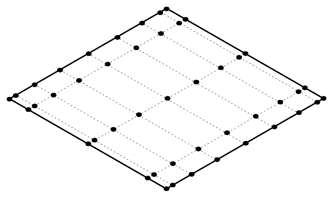
4.2. Wave Propagation in 2D Elements

The previous subsection shows that the TDSFEM can be used to efficiently model the phenomenon of mechanical wave propagation in one-dimensional elements. The changes in wave propagation may be successfully used to diagnose the analysed components. However, the excellent majority of technical devices requires more complex geometries to be used in the modelling process. The examples of modelling two-dimensional structures will be discussed here, in particular shell and plate elements designed and analysed with TDSFEM.

Multi-mode formulation of a higher order transversely deformable shell-type spectral finite element (SFE) for dynamic analysis of isotropic structures is presented and analysed in [135]. A method to generate the dispersion curves associated with the displacement fields obtained is presented by the authors, which utilises Hamilton’s principle and which leads to a set of associated equations of motion. These equations have been presented in the paper for the case of the analysed shell SFE as well as the dispersion curves resulting from them. The accuracy of the formulation proposed is assessed by comparison of dispersion curves obtained for the current model with dispersion curves obtained for exact solutions of the problem as well as comparison with shell theories well-known from the literature. Finally, in order to demonstrate the effectiveness of the current formulation of a higher order transversely deformable shell-type SFE, a series of numerical tests were performed. These comprised the analysis of natural frequencies and modes of vibration of an isotropic spherical shell as well as the wave propagation analysis in the case of the same spherical shell and a half-pipe shell-like structure. Combined application of TD-SFEM and the higher order transversely deformable shell SFE developed by the authors helps to reduce significantly modelling and discretisation errors of numerical investigation providing excellent accuracy, especially in comparison to the classical FEM and typical FEs commonly used for that purpose.

A TDSFEM deformed thin-walled spherical shell element for modal analysis and for an effective structural health monitoring technique based on propagation of guided elastic waves has been given in [87,136]. The first paper deals with certain problems related to static and modal analysis of isotropic shell structures representing a pressure vessel. The robustness and effectiveness of the spectral approach have been successfully demonstrated. Static and modal responses of the structure have been investigated by the use of transversally deformable shell-type spectral finite elements and the results of this investigation have been compared to known analytical solutions as well as those obtained by the use of commercially available software for the finite element method. The second paper takes advantage of the TDSFEM modelling technique in application to certain structural health monitoring (SHM) strategy. This has been realized based on results of numerical calculation and experimental investigations obtained with laser scanning vibrometry (LSV) and subsequent application of two different integral-based indices for damage quantification, these being the integral mean value (IMV) and the root mean square (RMS). Numerical tests by SFEM have been carried out for a square plate with through-hole damage, a cracked fuselage section with two stiffeners and a cracked wing section skin, all made out of aluminium. Experimental measurements by LSV included tests on a square aluminium plate, composite plate and a composite stabilizer of a PZL W-3A helicopter, all with simulated damage. During numerical and experimental investigations, damage sensitivity of both IMV and RMS indices was tested by considering various displacement components, signal time-scales or weighting factors. A certain practical method for quick construction of RMS damage maps based on experimental measurements by LSV has been also presented.

A novel formulation of a spectral plate element for wave propagation in isotropic structures is presented in [137]. In this formulation of the spectral plate finite element as approximation functions, Chebyshev polynomials of the first kind have been employed. The element makes use of on an extended form of the displacement field that enables one to investigate selectively or simultaneously both symmetric and anti-symmetric modes of Lamb waves propagating in plate structures. In addition, the dispersion relations associated with the extended displacement field have been presented and discussed in the paper. The effectiveness of the new spectral plate finite element has been illustrated on examples of propagation of elastic waves in a flat aluminium panel in the case of the fundamental symmetric and anti-symmetric modes of Lamb waves.

A pseudo-spectral Mindlin plate element with Chebyshev polynomials chosen as the elemental interpolating functions as they are proper for wave propagation modelling has been proposed by [138]. A diagonal system matrix has been obtained and therefore the equations of motion could be easily solved in the time domain by applying the central difference method of reducing the computational cost. Static, dynamic and elastic wave propagation problems have been analysed to obtain the efficiency of the proposed pseudo-spectral Mindlin plate element using two integration schemes for elemental stiffness matrix.

In [139], the authors have presented an interesting node distribution (Figure 3) for the proposed plate element model based on TDSFEM. The intention of these investigations has been the effective, computing time reducing simulation of Lamb wave propagation using methods for the numerical calculation. For this purpose, high-order shape functions and the Gauss–Lobatto–Legendre integration scheme has been introduced. Using the example of 2D plane strain plate elements, it has been shown that this method is able to provide an efficient analysis for the wave propagation in damaged and undamaged structures. The presented procedure has been verified by analytical computations as well as by alternatively obtained references.

Numerical analysis of physical phenomena occurring in elements of machines and devices requires a certain level of awareness of the differences between real structures and their numerical equivalents. For this reason, it is worth mentioning here the work on estimating numerical errors of specific modelling methods. Some research results concerned on this subject has been performed by [140]. In this work, the Legendre spectral finite elements have been examined through numerical experiments for static and dynamic Reissner–Mindlin plate bending and a mixed-quadrature scheme. Legendre spectral finite elements are high-order Lagrangian-interpolant finite elements with nodes located at the Gauss–Lobatto–Legendre quadrature points. Solutions on unstructured meshes have been examined in terms of accuracy as a function of the number of model nodes and total operations. While nodal-quadrature Legendre spectral finite elements have been shown elsewhere to be free of shear locking on structured grids, locking has been demonstrated on unstructured grids. Legendre spectral finite elements with mixed quadrature have been, however, locking free and are significantly more accurate than low-order finite-elements for a given model size or total computation time. An example of similar elements but regarding composite plates for static and dynamic deformation on unstructured grids has been analysed by [141]. The authors have analysed Legendre spectral finite elements application to Reissner–Mindlin composite plates. Nodal quadrature has been employed for mass-matrix calculations, and that has yield diagonal mass matrices. Full quadrature or mixed-reduced quadrature has been used for stiffness-matrix calculations. Solution accuracy has been examined in terms of model size, computation time, and memory storage for Legendre spectral finite elements and for quadratic serendipity elements calculated in a commercial finite-element code. Linear systems for both model types have been solved with the same sparse-system direct solver. At their best, Legendre spectral finite elements provide many orders of magnitude more accuracy than the quadratic elements for a fixed measure (e.g., computation time). At their worst, Legendre spectral finite elements provide the same accuracy as the quadratic elements for a given measure. The Legendre spectral finite elements have been insensitive to shear locking and were shown to be more robust in the thin-plate limit than their low-order counterparts.

As a type of composite material may be considered as media with solid and fluid layers, which is commonly used for marine seismic exploration. The data analysis of wave propagation in such media has been performed in [142]. In this paper, the authors have compared the accuracy of grid dispersion criteria and numerical examples based on methods like: the classical finite-difference method (FDM) based on the second-order displacement formulation of the elastic wave equation (DFDM), the staggered-grid finite difference method (SGFDM), the velocity-stress FDM with a standard grid (VSFDM) and the time domain spectral finite element method (TDSFEM). All of the considered methods yield limited accuracy for the surface waves because the proper boundary conditions are not incorporated into the numerical scheme. Overall, it has been demonstrated both by analytic treatment and numerical experiments, which a first-order velocity stress formulation can, in general, be used in dealing with fluid–solid interfaces without using staggered grids necessarily.

Functionally graded (FG) composite materials have been modelled by [143] where a cylinder subjected to an impulsive loading starting elastic wave propagation has been studied in detail. The displacement and stress distributions and the time histories of displacement and stress components have been obtained for various grading patterns. The results have shown that the compositional gradient exponent n does not have a distinct effect on the displacement or stress profiles but has an obvious influence on the wave travelling speed as well as the displacement and stress levels. The proposed method can be used to other types of axisymmetric FG structures like thick truncated cones and hollow cylinders, and also various loading and boundary conditions can be considered to these problems.

4.3. Wave Propagation in 3D Elements

3D elements, which should in fact be called solid elements, are useful in situations where complex fields of variables (displacement, deformation, electric potential, etc.) have to be modelled. In such cases, typically the three-dimensional theory of elasticity is applied. Thanks to TDSFEM modelling simplicity, it is relatively easy to derive it, especially for the analysis of elastic waves’ propagation. The important disadvantage of 3D analysis is that there are more degrees of freedom, which in turn leads to more calculation time [82].

The successful application of TDSFEM to the novel formulation of a 3D spectral element for wave propagation in reinforced concrete has been described here [144]. The reinforcement has been modelled as the truss spectral element and has been embedded in the 3D solid spectral finite element. Both elements have an equal number of nodes in the reinforcement direction and have the same number of degrees of freedom per each node. It has been assumed that there exists kinematic consistency between nodal displacements of the truss element and the solid element. This simplifying assumption has been justified by a linear character of wave propagation; however, this makes it impossible to diagnose material nonlinearities such as, for instance, de-bonding between steel and concrete. The developed 3D spectral element has been applied for modelling of wave propagation in reinforced concrete subjected to mechanical degradation. Different degradation models have been considered to reflect the real behaviour of bended beams. It has been shown that the models incorporating the uniform reduction of the beam stiffness worked well at the early stage of the degradation. The model with the distributed reduction of the stiffness enables for reflecting the behaviour of wave propagation at the stage, when macro-cracks are being developed. This model supports the possibility of the use of various spatial functions to analyse different stages of degradation. The formation of physical macro-cracks of large sizes in the more advanced phase of the bending process requires appropriate representation in the numerical model in the form of rows of nodes with a significantly reduced value of the Young’s modulus. The author declares that the results of the paper may be treated as pilot activities, requiring further work in this area.

Another 3D solid spectral element has been derived with shape functions based on Lagrange interpolation and Gauss–Lobatto–Legendre points here [145]. This particular approach has been applied for displacement approximation suited for fundamental modes of Lamb waves as well as potential distribution in piezoelectric transducers. A reliable numerical model of a transducer improves the quality of numerical analysis of any structural health monitoring algorithm. The novelty of the proposed research is the model geometry extension from flat to curved elements for application in shell-like structures. Exemplary visualisations of waves excited by the piezoelectric transducers in curved shell structure made of aluminium alloy have been presented. Simple signal analysis of wave interaction with a crack is performed. The crack is modelled by separation of appropriate nodes between elements. An investigation of influence of the crack length on wave propagation signals is performed. Additionally, some aspects of the spectral element method implementation have been discussed.

The importance of a reliable method of numerical modelling and simulations of PZT-induced Lamb wave propagation in plate-like structures has been also presented by [85]. The authors derive here a novel finite spectral plate element, which can efficiently model the three-dimensional behaviour of Lamb waves. In the formulation, linear displacement distributions in the thickness direction have been assumed for both the PZT layer and the base plate. A method to avoid the thickness locking has been proposed and used in the formulation. Two examples, one for the validation of the proposed spectral finite element and the other for the demonstration of crack detection in plates, have been presented and discussed. The contact between the two faces of crack has been considered. The discussion of numerical says that only the anti-symmetric mode is prone to thickness locking, thus a remedy should be made only on this part. The proposed spectral finite element can adequately model the Lamb wave propagation in plate-like structures and the complex scattering for the crack. Finally, the crack location can be well determined by a PZT-induced Lamb wave-based diagnosis algorithm.

A versatile character of the TDSFEM for modelling of different environments has been shown by [146], where the numerical simulation of acoustic waves in complex three-dimensional media has been proposed. This problems have been a subject of interest in many branches of science, from exploration geophysics to non-destructive testing and medical imaging. The article itself presents and validates a numerical technique based on an axisymmetric formulation of a TDSFEM in the time domain for heterogeneous fluid–solid media. Taking advantage of axisymmetry enables the study of relevant 3D configurations at a very moderate computational cost. The authors have presented and validated a numerical method based on time-domain spectral elements for coupled fluid solid full-wave propagation problems in an axisymmetric setting, including in cases with significant backscattering, which cannot be modelled, e.g., based on the parabolic equation approximation.

5. Discussion

The best summary of the literature analysis conducted will be a simple comparative example of selected numerical methods. For this purpose, the simplest structural element, i.e., a 1D rod made out of isotropic material with the parameters given in a Figure 4 has been chosen. This element has been modelled using three numerical methods—the classic FEM, FDSFEM and TDSFEM. The results of the numerical analysis are shown in Figure 5. In each of these cases, the rod has been excited by a 100 kHz carrier frequency signal. The excitation signal has been applied at one end of the rod, while the response has been recorded at the midpoint of the length of the element.

Thus, in the case of FEM, two options have been explored: a full inertia matrix and a diagonal one. As it can be noticed, the irresponsible use of FEM (the simplest two-node element) leads to significant errors. Those errors are the result of a numerical dispersion of the signal. In the response, the wave propagates either slower (in case of full inertia matrix) or faster (in case of diagonal inertia matrix). Naturally, these errors could be avoided by improving the mesh density or by using more advanced finite elements, or by using higher-order approximation functions. An interested reader is encouraged to follow some literature resources regarding this problem, like [82,130,131]. The second of the results discussed concerns the FDSFEM model. In this case, the correct time of signal propagation has been recorded, but no further reflections have occurred. This may be easily explained. In this method, a special throw-off element is applied at the opposite end to the excited one. This numerical activity eliminates the periodical feature of the Fourier transform, and, as its physical meaning is an energy conduit out of the system, there are no further internal boundary wave reflections. The third result presented concerns the application of TDSFEM. In this case, as a shape function, the Chebyshew polynomial of 6th order has been applied. As it can be seen from the diagram, for the time of occurrence in Figure 5, even in the simplest case, the signal is reproduced without any dispersion and appears exactly in the appropriate time windows (marked in each diagram as a grey background behind the signal). Therefore, it can be concluded that TDSFEM seems to be the most appropriate method for modelling the phenomenon of elastic wave propagation.

6. Conclusions

Regarding the literature review presented, the following conclusions can be drawn:

• both described spectral methods allow for a reduction in the calculation time compared to the analysis of the same more complex finite element geometries,
• the most often utilised FDSFEM modelling algorithm requires a simple and reverse Fourier transforms, which can lead to significant numerical errors in two-dimensional geometry, 3D example has not been found in the literature,
• the versatile nature of the TDSFEM is confirmed by the rapidly growing number of publications on the various examples of its use. This fact originates from the mathematical background of the method, i.e., non-uniform nodes distribution in the element modelled. This feature seems to be more effective for modelling problems where wave propagation in structures is considered,
• as stated in the literature [83], in the case of wave propagation modelling, the SEM reduces the computational memory by more than a factor of 20 in terms of total nodal numbers, compared with the FEM. Furthermore, the FEM costs more than 10 times the computational time, compared with the SEM,
• the error is reduced when the average distance between nodes (TDSFEM) becomes shorter [84].

The author of this review is aware of the limited number of quoted works; however, attention should be paid to the purpose of this paper, which is to specify differences in two spectral approaches and the benefits and limitations of these differences resulting from them in terms of wave propagation analysis in the field of damage detection. Although the topic of modelling wave propagation by spectral methods is interesting, the author is aware of a limited number of research centres dealing with this problem. It was not the intention of the author to specifically exclude anyone who deals with this complicated area of mathematical interest.

References

1. Hall, S. The effective management and use of structural health data. In Proceedings of the 2nd International Workshop on Structural Health Monitoring, Stanford, CA, USA, 8–10 September 1999; pp. 265–275. [Google Scholar]
2. Inman, D.; Farrar, C.; Lopes, V., Jr.; Steffen, V., Jr. (Eds.) Damage Prognosis for Aerospace, Civil and Mechanical Systems; Wiley: Hoboken, NJ, USA, 2005. [Google Scholar]
3. Kleiber, M.; Burczyński, T.; Wilde, K.; Górski, J.; Winkelmann, K.; Smakosz, L. (Eds.) Advances in Mechanics. Theoretical, Computational and Interdisciplinary Issues; CRC Press: Boca Raton, FL, USA, 2016. [Google Scholar]
4. Kessler, S.; Spearing, S.; Soutis, C. Damage detection in composite materials using Lamb wave methods. Smart Mater. Struct. Struct. 2002, 11, 269–278. [Google Scholar] [CrossRef] [Green Version]
5. Farrar, C.; Doebling, S. An Overview of Modal-Based Damage Identification Methods; Technical Report; Los Alamos National Laboratory: Los Alamos, NM, USA, 1997.
6. Doebling, S.; Farrar, C.; Prime, M. A Summary Review of Vibration-based Damage Identification Methods. Shock Vib. Dig. 1998, 30, 91–105. [Google Scholar] [CrossRef]
7. Israr, A.; Cartmell, M.; Krawczuk, M.; Ostachowicz, W.; Manoach, E.; Trendafilova, I.; Shishkina, E.; Palacz, M. On approximate anatytical solutions for vibrations in cracked plates. Appl. Mech. Mater. 2006, 5–6, 315–322. [Google Scholar] [CrossRef]
8. Raja, S.; Prathima Adya, H.; Viswanath, S. Analysis of Piezoelectric Composite Beam and Plate with Multiple Delaminations. Struct. Health Monit. 2006, 5, 255–266. [Google Scholar] [CrossRef]
9. Wang, J.; Qiao, P. Improved Damage Detection for Beam-type Structures using a Unigorm Load Surface. Struct. Health Monit. 2007, 6, 99–110. [Google Scholar] [CrossRef]
10. Sinou, J. Mechanical Vibrations: Measurement, Effects and Control; chapter A Review of Damage Detection and Health Monitoring of Mechanical Systems from Changes in the Measurement of Linear and Non-linear Vibrations; Nova Science Publishers: Hauppauge, NY, USA, 2009; pp. 643–702. [Google Scholar]
11. Fan, W.; Qiao, P. Vibration-based Damage Identification Methods: A Review and Comparative Study. Struct. Health Monit. 2011, 10, 83–111. [Google Scholar] [CrossRef]
12. Wang, C.S.; Wu, F.; Chang, F. Structural Health Monitoring from fiber-reinforced ccomposite to steel-reinforced concrete. Smart Mater. Struct. 2001, 10, 548–551. [Google Scholar] [CrossRef]
13. Su, Z.; Ye, L. Fundamental Lamb Mode-based Delamination Detection for CF/EP Composite Laminates Using Distributed Piezoelectrics. Struct. Health Monit. 2004, 3, 43–68. [Google Scholar] [CrossRef]
14. Mal, A.; Ricci, F.; Banerjee, S.; Shih, F. A Conceptual Structural Health Monitoring System based on Vibration and Wave Propagation. Struct. Health Monit. 2005, 4, 283–293. [Google Scholar] [CrossRef]
15. Lestari, W.; Qiao, P. Application of Wave Propagation Analysis for Damage Identification in Composite Laminated Beams. Compos. Mater. 2005, 39, 1967–1984. [Google Scholar] [CrossRef]
16. Monnier, T. Lamb Waves-based Impact Damage Monitoring of a Stiffened Aircraft Panel using Piezoelectric Transducers. J. Intell. Mater. Syst. Struct. 2006, 17, 411–421. [Google Scholar] [CrossRef]
17. Su, Z.; Ye, L.; Lu, Y. Guided Lamb waves for identification of damage in composite structures: A review. J. Sound Vib. 2006, 295, 753–780. [Google Scholar] [CrossRef]
18. Song, G.; Gu, H.; Mo, Y.; Hsu, T.T.C.; Dhonde, H. Concrete structural health monitoring using embedded piezoceramic transducers. Smart Mater. Struct. 2007, 16, 959–968. [Google Scholar] [CrossRef]
19. Park, H.; Sohn, H.; Law, K.; Farrar, C.R. Time reversal active sensing for health monitoring of a composite plate. J. Sound Vib. 2007, 302, 50–66. [Google Scholar] [CrossRef]
20. Raghavan, A.; Cesnik, C. Review of Guided-wave Structural Health Monitoring. Shock Vib. Dig. 2007, 39, 91–114. [Google Scholar] [CrossRef]
21. Grabowska, J.; Palacz, M.; Krawczuk, M.; Ostachowicz, W.; Trendafilova, I.; Manoach, E.; Cartmell, M. Wavelet analysis for damage identification in composite structures. Key Eng. Mater. 2007, 347, 253–258. [Google Scholar] [CrossRef]
22. Grabowska, J.; Palacz, M.; Krawczuk, M. Damage identification by wavelet analysis. Mech. Syst. Signal Process. 2008, 22, 1623–1635. [Google Scholar] [CrossRef]
23. Ng, C.; Veidt, M.; Lam, H. Guided wave damage characterisation in beams utilising probabilistic optimisation. Eng. Struct. 2009, 31, 2842–2850. [Google Scholar] [CrossRef] [Green Version]
24. Joglekar, D.M.; Mitra, M. Nonlinear analysis of flexural wave propagation through 1D waveguides with a breathing crack. J. Sound Vib. 2015, 344, 242–257. [Google Scholar] [CrossRef]
25. Sridaran Venkat, R.; Rathod, V.; Mahapatra, D.; Boller, C. Simulation von Sensorsystemen zur Inspektion von Bauteilstrukturen im Sinne eines Structural Health Monitoring. In Proceedings of the Annual Conference of German Society for Non-Destructive Testing (DGZFP), Salzburg, Austria, 11–13 May 2015; pp. 1–8. [Google Scholar]
26. Mitra, M.; Gopalakrishnan, S. Guided wave based structural health monitoring: A review. Smart Mater. Struct. 2016, 25, 1–28. [Google Scholar] [CrossRef]
27. Nazeer, N.; Ratassepp, M.; Fan, Z. Damage detection in bent plates using shear horizontal guided waves. Ultrasonics 2017, 75, 155–163. [Google Scholar] [CrossRef] [PubMed]
28. Yu, Y.; Yan, N. Numerical Study on Guided Wave Propagation in Wood Utility Poles: Finite Element Modelling and Parametric Sensitivity Analysis. Appl. Sci. 2017, 7, 1063. [Google Scholar] [Green Version]
29. Martinez, M.; Pant, S.; Yanishevsky, M.; Backman, D. Residual stress effects of a fatigue crack on guided Lamb waves. Smart Mater. Struct. 2017, 26, 1–16. [Google Scholar] [CrossRef]
30. Kudela, P.; Radzieński, M.; Ostachovicz, W.; Yang, Z. Structural Health Monitoring system based on a concept of Lamb wave focusing by the piezoelectric array. Mech. Syst. Signal Process. 2018, 108, 21–23. [Google Scholar] [CrossRef]
31. Giurgiutiu, V.; Zagrai, A. Damage Detection in Thin Plates and Aerospace Structures with the Electro-Mechanical Impedance Method. Struct. Health Monit. 2005, 4, 99–118. [Google Scholar] [CrossRef] [Green Version]
32. Dhakal, D.; Neupane, K.; Thapa, C.; Ramanjaneyulu, G. Different techniques of structural health monitoring. Int. J. Civ. Struct. Infrastruct. Eng. Res. Dev. 2013, 3, 55–66. [Google Scholar]
33. Ludwig, R.; Lord, W. Afbeams-element formulation for the study of ultrasonic NDT systems. IEEE Trans. Ultrason. Ferroelectr. Freq. Control 1988, 35, 809–820. [Google Scholar] [CrossRef] [PubMed]
34. Kishore, N.; Sridhar, I.; Iyengar, N. Finite element modelling of the scattering of ultrasonic waves by isolated flaws. NDT E Int. 2000, 33, 297–305. [Google Scholar] [CrossRef]
35. Shah, S.; Popovics, J.; Subramaniam, K.; Aldea, C. New Directions in Concrete Health Monitoring Technology. J. Eng. Mech. 2000, 126, 754–760. [Google Scholar] [CrossRef]
36. Rizzo, P.; Lanza di Scalea, F. Feature Extraction for Defect Detection in Strands by Guided Ultrasonic Waves. Struct. Health Monit. 2006, 5, 297–308. [Google Scholar] [CrossRef]
37. Broda, D.; Staszewski, W.; Martowicz, A.; Uhl, T.; Silberschmidt, V. Modelling of nonlinear crack-wave interactions for damage detection based on ultrasound—A review. J. Sound Vib. 2014, 333, 1097–1118. [Google Scholar] [CrossRef]
38. Ravi, N.; Rathod, V.; Chakraborty, N.; Mahapatra, D.R.; Sridaran, R.; Boller, C. Modeling ultrasonic NDE and guided wave based structural health monitoring. In Proceedings of the Structural Health Monitoring and Inspection of Advanced Materials, Aerospace, and Civil Infrastructure, San Diego, CA, USA, 9–12 March 2015. [Google Scholar]
39. Murayama, H.; Kageyama, K.; Naruse, H.; Shimada, A.; Uzawa, K. Application of Fiber-Optic Distributed Sensors to Health Monitoring for Full-Scale Composite Structures. J. Intell. Mater. Syst. Struct. 2003, 14, 3–13. [Google Scholar] [CrossRef]
40. Giurgiutiu, V.; Cuc, C. Embedded Non-destructive Evaluation for Structural Health Monitoring, Damage Detection, and Failure Prevention. Shock Vib. Dig. 2005, 37, 83–105. [Google Scholar] [CrossRef]
41. Montalvao, D.; Maia, N.; Ribeiro, A. A Review of Vibration-based Structural Health Monitoring with Special Emphasis on Composite Materials. Shock Vib. Dig. 2006, 38, 295–324. [Google Scholar] [CrossRef] [Green Version]
42. Reda Taha, M.; Noureldin, A.; Lucero, J.; Baca, T. Wavelet Transform for Structural Health Monitoring: A Compendium of Uses and Features. Struct. Health Monit. 2006, 5, 267–295. [Google Scholar] [CrossRef]
43. Nichols, J.; Trickey, S.; Seaver, M.; Moniz, L. Use of Fiber-optic Strain Sensors and Holder Exponents for Detecting and Localizing Damage in an Experimental Plate Structure. J. Intell. Mater. Syst. Struct. 2007, 18, 51–67. [Google Scholar] [CrossRef]
44. Boller, C.; Chang, F.; Fujino, Y. (Eds.) Encyclopedia of Structural Health Monitoring; John Wiley and Sons: Hoboken, NJ, USA, 2009. [Google Scholar]
45. Gopalakrishnan, S.; Chakraborty, A.; Roy Mahapatra, R. Spectral Finite Element Method; Springer: London, UK, 2008. [Google Scholar]
46. Ham, S.; Bathe, K. A finite element method enriched for wave propagation problems. Comput. Struct. 2012, 94–95, 1–12. [Google Scholar] [CrossRef]
47. Jaleel, K.; Kishore, N.; Sundararajan, V. Finite-element simulation of elastic wave propagation in orthotropic composite materials. Mater. Eval. 1993, 51, 830–838. [Google Scholar]
48. Komijani, M.; Gracie, R. An enriched finite element model for wave propagation in fractured media. Finite Elem. Anal. Des. 2017, 125, 14–23. [Google Scholar] [CrossRef]
49. Simonetti, F.; Cawley, P. On the nature of shear horizontal wave propagation in elastic plates coated with viscoelastic materials. Proc. R. Soc. A 2004, 204, 2197–2221. [Google Scholar] [CrossRef]
50. Cheney, E. Introduction to Approximation Theory; McGraw-Hill: New York, NY, USA, 1966. [Google Scholar]
51. Rivlin, T. An Introduction to the Approximation of Functions; Blaisdell Publishing Co.: Toronto, ON, Canada, 1969. [Google Scholar]
52. Trefethen, L. Approximation Theory and Approximation Practice; SIAM: Philadelphia, PA, USA, 2013. [Google Scholar]
53. Pinkus, A. Weierstrass and approximation Theory. J. Approx. Theory 2000, 107, 1–66. [Google Scholar] [CrossRef]
54. Sneddon, I. Fourier Transform; McGraw-Hill: New York, NY, USA, 1951. [Google Scholar]
55. Sneddon, I. Elements of Partial Differential Equations; Dover Publications, Inc.: Mineola, NY, USA, 2006. [Google Scholar]
56. Conway, H.; Jakubowski, M. Axial impact of short cylindrical bars. J. Appl. Mech. 1969, 36, 809–813. [Google Scholar] [CrossRef]
57. Davies, R. Acritbars study of the Hopkinson pressure bar. Philos. Trans. R. Soc. 1948, 240, 375–457. [Google Scholar] [CrossRef]
58. Hsieh, D.; Kolsky, H. An experimental study of pulse propagation in elastic cylinders. Proc. Philos. Soc. 1958, 71, 608–612. [Google Scholar] [CrossRef]
59. Cooley, J.; Turkey, J. An algorithm for the machine calculation of complex Fourier series. Math. Comput. 1965, 19, 297–301. [Google Scholar] [CrossRef]
60. Wikipedia, N. Solution methods of numerical partial differential equations. Wikipedia Internet Resour. 2018, 1, 1–2. [Google Scholar]
61. Willberg, C.; Duczek, S.; Vivar-Perez, J.; Ahmad, Z. Simulation Methods for Guided Wave-Based Structural Health Monitoring: A Review. Appl. Mech. Rev. 2015, 67, 010803. [Google Scholar] [CrossRef] [Green Version]
62. Shizgal, B. Spectral Methods in Chemistry and Physics. Applications to Kinetic Theory and Quantum Mechanics; Springer Science+Business Media: Dordrecht, The Netherlands, 2015. [Google Scholar]
63. Gottlieb, D.; Orszag, S. Numerical Analysis of Spectral Methods: Theory and Applications; SIAM-CBMS: Philadelphia, PA, USA, 1977. [Google Scholar]
64. Clouteau, D.; Cottereau, R.; Lombaert, G. Dynamics of structures coupled with elastic media—A review of numerical models and methods. J. Sound Vib. 2013, 332, 2415–2436. [Google Scholar] [CrossRef] [Green Version]
65. Karniadakis, G.; Sherwin, S. Spectral/hp Element Methods for Computational Fluid Dynamics; Oxford University Press: Oxford, UK, 2005. [Google Scholar]
66. Gopalakrishnan, S.; Mitra, M. Wavelet Methods for Dynamical Problems; CRC Press: Boca Raton, FL, USA, 2010. [Google Scholar]
67. Akhras, G.; Li, W. Stability and free vibration analysis of thick piezoelectric composite plates using spline finite strip method. Int. J. Mech. Solids 2011, 53, 575–584. [Google Scholar] [CrossRef]
68. Mitra, M.; Gopalakrishnan, S. Spectrally formulated wavelet finite element for wave propagation and impact force identification in connected 1D waveguides. Int. J. Solids Struct. 2005, 42, 4695–4721. [Google Scholar] [CrossRef]
69. Mitra, M.; Gopalakrishnan, S. Extraction of wave characteristics from wavelet-based spectral finite element formulation. Mech. Syst. Signal Process. 2006, 20, 2046–2079. [Google Scholar] [CrossRef]
70. Mitrou, G.; Ferguson, N.; Renno, J. Wave transmission through two-dimensional structures by the hybrid FE/WFE approach. J. Sound Vib. 2017, 389, 484–501. [Google Scholar] [CrossRef] [Green Version]
71. Waki, Y.; Mace, B.; Brennan, M. Numerical issues concerning the wave and finite element method for free and forced vibrations of waveguides. J. Sound Vib. 2009, 327, 92–108. [Google Scholar] [CrossRef]
72. Shen, Y.; Giurgiutiu, V. Effective non-reflective boundary for Lamb waves: Theory, finite element implementation, and applications. Wave Motion 2015, 58, 22–41. [Google Scholar] [CrossRef] [Green Version]
73. Shen, Y.; Cesnik, C. Modeling of nonlinear interactions between guided waves and fatigue cracks using local interaction simulation approach. Ultrasonics 2017, 74, 106–123. [Google Scholar] [CrossRef] [PubMed]
74. Sad Saoud, K.; Le Grognec, P. A unified formulation for the biaxial local and global buckling analysis of sandwich panels. Thin-Walled Struct. 2014, 82, 13–23. [Google Scholar] [CrossRef]
75. Takei, A.; Brau, F.; Roman, B.; Bico, J. Stretch-induced wrinkles in reinforced membranes: From out-of-plane to in-plane structures. Europhys. Lett. 2011, 96, 64001. [Google Scholar] [CrossRef] [Green Version]
76. Wang, X.; So, R. Timoshenko beam theory: A perspective based on the wave-mechanics approach. Wave Motion 2015, 57, 64–87. [Google Scholar] [CrossRef]
77. Faccioli, E.; Maggio, F.; Paolucci, R.; Quarteroni, A. 2D and 3D elastic wave propagation by a pseudo-spectral domain decomposition method. J. Seismol. 1997, 1, 237–251. [Google Scholar] [CrossRef]
78. Pau, A.; Achillopoulou, D.; Vestroni, F. Scattering of guided shear waves in plates with discontinuities. NDT E Int. 2016, 84, 67–75. [Google Scholar] [CrossRef]
79. Doyle, J. Wave Propagation in Structures. Spectral Analysis Using Fast Discrete Fourier Transforms, 2nd ed.; Springer: New York, NY, USA, 1997. [Google Scholar]
80. Rekatsinas, C.S.; Nastos, C.V.; Theodosiou, T.C.; Saravanos, D.A. A time-domain high-order spectral finite element for the simulation of symmetric and antisymmetric guided waves in laminated composite strips. Wave Motion 2015, 53, 1–19. [Google Scholar] [CrossRef]
81. Kudela, P.; Żak, A.; Krawczuk, M.; Ostachovicz, W. Modelling of wave propagation in composite plates using the time domain spectral element method. J. Sound Vib. 2007, 302, 728–745. [Google Scholar] [CrossRef]
82. Ostachowicz, W.; Kudela, P.; Krawczuk, M.; Żak, A. Guided Waves in Structures for SHM: The Time-Domain Spectral Element Method; Wiley and Sons: West Sussex, UK, 2012. [Google Scholar]
83. Kim, Y.; Ha, S.; Chang, F.K. Time-domain spectral element method for build-in piezoelectric-actuator-induced Lamb wave propagation analysis. AIAA J. 2008, 46, 591–600. [Google Scholar] [CrossRef]
84. Ha, S.; Chang, F.K. Optimizing a spectral element for modeling PZT-induced Lamb wave propagation in thin plates. Smart Mater. Struct. 2010, 19, 015015. [Google Scholar] [CrossRef]
85. Ge, L.; Wang, X.; Jin, C. Numerical modeling of PZT induced Lamb wave-based crack detection in plate-like structures. Wave Motion 2014, 51, 867–885. [Google Scholar] [CrossRef]
86. Peng, H.; Meng, G.; Li, F. Modeling of wave propagation in plate structures using three-dimensional spectral element method for damage detection. J. Sound Vib. 2009, 320, 942–954. [Google Scholar] [CrossRef]
87. Żak, A.; Radzieński, M.; Krawczuk, M.; Ostachovicz, W. Damage detection strategies based on propagation of guided elastic waves. Smart Mater. Struct. 2012, 21, 1–18. [Google Scholar] [CrossRef]
88. Schulte, R.T.; Fritzen, C.P.; Moll, J. Spectral element modelling of wave propagation in isotropic and anisotropic shell-structures including different types of damage. In Conference Series: Material Science and Engineering; IOP Publishing: Bristol, UK, 2010; pp. 1–10. [Google Scholar]
89. Rucka, M. Modelling of in-plane wave propagation in a plate using spectral element method and Kane-Mindlin theory with application to damage detection. Arch. Appl. Mech. 2011, 81, 1877–1888. [Google Scholar] [CrossRef]
90. Patera, A. A Spectral Element Method for Fluid Dynamics: Laminar Flow in a Channel Expansion. J. Comput. Phys. 1984, 54, 468–488. [Google Scholar] [CrossRef]
91. Timmermans, L. Analysis of Spectral Element Methods with Application to Incompressible Flow. Ph.D. Thesis, Eindhoven University of Technology, Eindhoven, The Netherlands, 1994. [Google Scholar]
92. Komatitsch, D.; Vilotte, J. The spectral element method: An efficient tool to simulate the seismic response of 2D and 3D geological structures. Bull. Seismol. Soc. Am. 1998, 88, 368–392. [Google Scholar]
93. Komatitsch, D.; Vilotte, J.; Vai, R.; Castillo-Covarrubias, J.; Sanchez-Sesma, F. The spectral element method for elastic wave equations-application to 2D and 3D seismic problems. Int. J. Numer. Methods Eng. 1999, 45, 1139–1164. [Google Scholar] [CrossRef]
94. Komatitsch, D.; Barnes, C.; Tromp, J. Simulation of anisotropic wave propagation based upon a spectral element method. Geophysics 2000, 65, 1251–1260. [Google Scholar] [CrossRef]
95. Lee, U.; Kim, J.; Leung, A. The spectral element method in structural dynamics. Shock Vib. 2000, 32, 451–465. [Google Scholar] [CrossRef]
96. Seriani, G.; Oliveira, S. Dispersion analysis of spectral element methods for elastic wave propagation. Wave Motion 2008, 45, 729–744. [Google Scholar] [CrossRef]
97. Zhong, W.; Howson, W.; Williams, F. Precise solutions for surface wave propagation in stratified material. J. Vib. Acoust. 2001, 123, 198–204. [Google Scholar] [CrossRef]
98. Cho, J.; Lee, U. An FFT-based spectral analysis method for linear discrete dynamic systems with non-proportional damping. Shock Vib. 2006, 13, 595–606. [Google Scholar] [CrossRef]
99. Chakraborty, A.; Gopalakrishnan, S. A spectral finite element model for wave propagation analysis in laminated composite plate. J. Vib. Acoust. 2006, 128, 477–488. [Google Scholar] [CrossRef]
100. Virieux, J.; Calandra, H.; Plessix, R. A review of the spectral, pseudo-spectral, finite-difference and finite-element modelling techniques for geophysical imaging. Geophys. Prospect. 2011, 59, 794–813. [Google Scholar] [CrossRef]
101. Krawczuk, M.; Grabowska, J.; Palacz, M. Longitudinal wave propagation. Part I-Comparison of rod theories. J. Sound Vib. 2006, 295, 461–478. [Google Scholar] [CrossRef]
102. Krawczuk, M.; Grabowska, J.; Palacz, M. Longitudinal wave propagation. Part II-Analysis of crack influence. J. Sound Vib. 2006, 295, 479–490. [Google Scholar] [CrossRef]
103. Palacz, M.; Krawczuk, M.; Ostachowicz, W. Detection of additional mass in rods: Experimental and numerical investigation. Arch. Appl. Mech. 2005, 74, 820–826. [Google Scholar] [CrossRef]
104. Gopalakrishnan, S.; Doyle, J. Spectral super-elements for wave propagation in structures with local non-uniformities. Comput. Methods Appl. Mech. Eng. 1995, 121, 77–90. [Google Scholar] [CrossRef]
105. Machado, M.; Adhikari, S.; Dos Dantos, J. A spectral approach for damage quantification in stochastic dynamic systems. Mech. Syst. Signal Process. 2017, 88, 253–273. [Google Scholar] [CrossRef]
106. Wang, Y.; Hao, H.; Zhu, X.; Ou, J. Spectral Element Modelling of Wave Propagation with Boundary and Structural Discontinuity Reflections. Adv. Struct. Eng. 2012, 15, 855–870. [Google Scholar] [CrossRef]
107. Lee, U. Spectral Element Method in Structural Dynamics; John Wiley &Sons (Asia) Pte Ltd.: Singapore, 2009. [Google Scholar]
108. Palacz, M.; Krawczuk, M. Analysis of longitudinal wave propagation in a cracked rod by the spectral element method. Comput. Struct. 2002, 80, 1809–1816. [Google Scholar] [CrossRef]
109. Krawczuk, M.; Palacz, M.; Ostachowicz, W. Spectral Plate Element for Crack Detection with the Use of Propagating Waves. Mater. Sci. Forum 2003, 440–441, 187–194. [Google Scholar] [CrossRef]
110. Krawczuk, M.; Palacz, M.; Ostachowicz, W. The dynamic analysis of a cracked Timoshenko beam by the spectral element method. J. Sound Vib. 2003, 264, 1139–1153. [Google Scholar] [CrossRef]
111. Ostachowicz, W.; Krawczuk, M.; Palacz, M. Detection of delamination in multilayer composite beams. Key Eng. Mater. 2003, 245–246, 483–490. [Google Scholar] [CrossRef]
112. Palacz, M.; Krawczuk, M.; Ostachowicz, W. The spectral finite element model for analysis of flexural-shear coupled wave propagation. Part 2: Delaminated multilayer composite beam. Compos. Struct. 2005, 68, 45–51. [Google Scholar] [CrossRef]
113. Palacz, M.; Krawczuk, M.; Ostachowicz, W. The spectral finite element model for analysis of flexural-shear coupled wave propagation. Part 1: Laminated multilayer composite beam. Compos. Struct. 2005, 68, 37–44. [Google Scholar] [CrossRef]
114. Wang, Y.; Zhu, X.; Hao, H.; Ou, J. Guided wave propagation and spectral element method for debonding damage assesment in RC structures. J. Sound Vib. 2009, 324, 751–772. [Google Scholar] [CrossRef]
115. Sarvestan, V.; Mirdamadi, H.; Ghayour, M. Vibration analysis of cracked Timoshenko beam under moving load with constant velocity and acceleration by spectral finite element method. Int. J. Mech. Sci. 2017, 122, 318–330. [Google Scholar] [CrossRef]
116. Chakraborty, A.; Gopalakrishnan, S. A spectrally formulated finite element for wave propagation analysis in functionally graded beams. Int. J. Solids Struct. 2003, 40, 2421–2448. [Google Scholar] [CrossRef]
117. Chakraborty, A.; Gopalakrishnan, S. A higher-order spectral element for wave propagation analysis in functionally graded materials. Acta Mech. 2004, 172, 17–43. [Google Scholar] [CrossRef]
118. Joglekar, D.M.; Mitra, M. Analysis of flexural wave propagation through beams with a breathing crack using wavelet spectral finite element method. Mech. Syst. Signal Process. 2016, 76, 576–591. [Google Scholar] [CrossRef]
119. Ajith, V.; Gopalakrishnan, S. Wave propagation in a porous composite beam: Porosity determination, location and quantification. Int. J. Solids Struct. 2013, 50, 556–569. [Google Scholar] [CrossRef]
120. Ahmida, K.; Arruda, J. On the relation between complex modes and wave propagation phenomena. J. Sound Vib. 2002, 255, 663–684. [Google Scholar] [CrossRef]
121. Ruzzene, M.; Hanagud, S. Computational Techniques for Structural Health Monitoring; chapter Spectral Finite Element Method; Springer: London, UK, 2011; pp. 177–217. [Google Scholar]
122. Amaratunga, K.; Wiliams, J. Time integration using wavelet. In Proceedings of the SPIE, Wavelet Application for Dual Use, Orlando, FL, USA, 17–21 April 1995; Volume 2491, pp. 894–902. [Google Scholar]
123. Amaratunga, K.; Wiliams, J. Wavelet-Galerkin solution of boundary valur problems. Arch. Comput. Methods Eng. 1997, 4, 234–285. [Google Scholar] [CrossRef]
124. Williams, J.; Amaratunga, K. A discrete wavelet transform without edge effects using wavelet extrapolation. J. Fourier Anal. Appl. 2003, 3, 435–449. [Google Scholar] [CrossRef]
125. Wang, G.; Unal, A. Free vibration of stepped thicthick rectangular plates using spectral finite element method. J. Sound Vib. 2013, 332, 4324–4338. [Google Scholar] [CrossRef]
126. Park, I.; Kim, T.; Lee, U. Frequency Domain Spectral Element Model for the Vibration Analysis of a Thin Plate with Arbitrary Boundary Conditions. Math. Probl. Eng. 2016, 2016, 1–21. [Google Scholar] [CrossRef]
127. Bahrami, S.; Shirmohammadi, F.; Saadatpour, M. Vibration analysis of thin shallow shell using spectral element method. Appl. Math. Model. 2017, 44, 470–480. [Google Scholar] [CrossRef]
128. Boyd, J. Chebyshew and Fourier Spectral Methods; Dover Publications, Inc.: Mineola, NY, USA, 2000. [Google Scholar]
129. Rucka, M. Guided Wave Propagation in Structures. Modelling, Experimental Studies and Application to Damage Detection; Politechnika Gdańska: Gdańska, Poland, 2011. [Google Scholar]
130. Żak, A.; Krawczuk, M. Assessment of rod behaviour theories used in spectral finite element modelling. J. Sound Vib. 2010, 329, 2099–2113. [Google Scholar] [CrossRef]
131. Żak, A.; Krawczuk, M. Certain numerical issues of wave propagation modelling in rods by the Spectral Finite Element Method. Finite Elem. Anal. Des. 2011, 47, 1036–1046. [Google Scholar] [CrossRef]
132. Rucka, M. Experimental and numerical studies of guided wave damage detection in bars with structural discontinuities. Arch. Appl. Mech. 2010, 80, 1371–1390. [Google Scholar] [CrossRef]
133. Żak, A.; Krawczuk, M. Assessment of flexural beam behaviour theories used for dynamics and wave propagation problems. J. Sound Vib. 2012, 331, 5715–5731. [Google Scholar] [CrossRef]
134. Rucka, M. Experimental and numerical study on damage detection in an L-joint using guided wave propagation. J. Sound Vib. 2010, 329, 1760–1779. [Google Scholar] [CrossRef]
135. Żak, A.; Krawczuk, M. A higher order transversely deformable shell-type spectral finite element for dynamic analysis of isotropic structures. Finite Elem. Anal. Des. 2018, 142, 17–29. [Google Scholar] [CrossRef]
136. Żak, A.; Krawczuk, M. Static and dynamic analysis of isotropic shell structures by the spectral finite element method. Mod. Pract. Stress Vib. Anal. 2012, 382, 1–6. [Google Scholar] [CrossRef]
137. Żak, A. A novel formulation of a spectral plate element for wave propagation in isotropic structures. Finite Elem. Anal. Des. 2009, 45, 650–658. [Google Scholar] [CrossRef]
138. Liu, Y.; Hu, N.; Yan, C.; Peng, X.; Yan, B. Construction of a Mindlin pseudospectral plate element and evaluating efficiency of the element. Finite Elem. Anal. Des. 2009, 45, 538–546. [Google Scholar] [CrossRef]
139. Hennings, B.; Lammering, R.; Gabbert, U. Numerical simulation of wave propagation using spectral finite elements. CEAS Aeronaut J. 2013, 4, 3–10. [Google Scholar] [CrossRef]
140. Brito, K.; Sprague, M. Reissner-Mindlin Legendre spectral finite elements with mixed reduced quadrature. Finite Elem. Anal. Des. 2012, 58, 74–83. [Google Scholar] [CrossRef]
141. Sprague, M.; Purkayastha, A. Legendre spectral finite element for Reissner-Mindlin composite plates. Finite Elem. Anal. Des. 2015, 105, 33–43. [Google Scholar] [CrossRef]
142. De Basabe, J.; Sen, M. A comparison of finite-difference and spectral-element methods for elastic wave propagation in media with a fluid–solid interface. Geophys. J. Int. 2015, 200, 278–298. [Google Scholar] [CrossRef]
143. Xu, C.; Yu, Z. Numerical simulation of elastic wave propagation in functionally graded cylinders using time-domain spectral finite element method. Adv. Mech. Eng. 2017, 9, 1–17. [Google Scholar] [CrossRef]
144. Rucka, M.; Witkowski, W.; Chróścielewski, J.; Burzyński, S.; Wilde, K. A novel formulation of 3D spectral element for wave propagation in reinforced concrete. Bull. Pol. Acad. Sci. Tech. Sci. 2017, 65, 805–813. [Google Scholar] [CrossRef] [Green Version]
145. Ostachowicz, W.; Kudela, P. Wave Propagation Numerical Models in Damage Detection Based in the Tine Domain Spectral Element Method. In IOP Conference Series: Materials Science and Engineering; IOP Publishing: Bristol, UK, 2010; Volume 10, pp. 1–10. [Google Scholar]
146. Bottero, A.; Cristini, P.; Komatitsch, D. An axisymmetric time-domain spectral-element method for full-wave simulations: Application to ocean acoustics. J. Acoust. Soc. Am. 2016, 140, 3520–3530. [Google Scholar] [CrossRef] [PubMed] [Green Version]
147. Samaratunga, D.; Jha, R.; Gopalakrishnan, S. Wavelet spectral finite element for wave propagation in shear deformable laminated composite plates. Compos. Struct. 2014, 108, 341–353. [Google Scholar] [CrossRef]
148. Samaratunga, D.; Jha, R.; Gopalakrishnan, S. Wavelet spectral finite element for modeling guided wave propagation and damage detection in stiffened composite panels. Struct. Health Monit. 2016, 15, 317–334. [Google Scholar] [CrossRef]
149. Khalili, A.; Samaratunga, D.; Jha, R.; Lacy, T.; Gopalakrishnan, S. Wavelet Spectral Finite Element Based User-Defined Element in ABAQUS for Modeling Delamination in Composite Beams. In Proceedings of the 23rd AIAA/AHS Adaptive Structures Conference, Kissimmee, FL, USA, 5–9 January 2015. [Google Scholar]
150. Khalili, A.; Jha, R.; Samaratunga, D. The Wavelet Spectral Finite Element-based user-defined element in Abaqus for wave propagation in one-dimensional composite structures. Trans. Soc. Model. Simul. Int. 2017, 93, 1–10. [Google Scholar] [CrossRef]
Figure 1. Flow diagram for a signal reconstruction procedure with FDSFEM.
Applsci 08 01124 g001
Figure 2. Exemplary node distribution in TDSFEM element formulation.
Applsci 08 01124 g002
Figure 3. A node distribution in the plate element proposed by [139].
Applsci 08 01124 g003
Figure 4. Exemplary rod element, no model dispersion, 161 degrees of freedom.
Applsci 08 01124 g004
Figure 5. Errors resulting from numerical discretisation.
Applsci 08 01124 g005