Evaluating the Effects of Steel Fibers on Mechanical Properties of Ultra-High Performance Concrete Using Artificial Neural Networks

Abstract
:Featured Application
Abstract
1. Introduction
2. Artificial Neural Network Approach
3. Database and Models
3.1. Data Collection
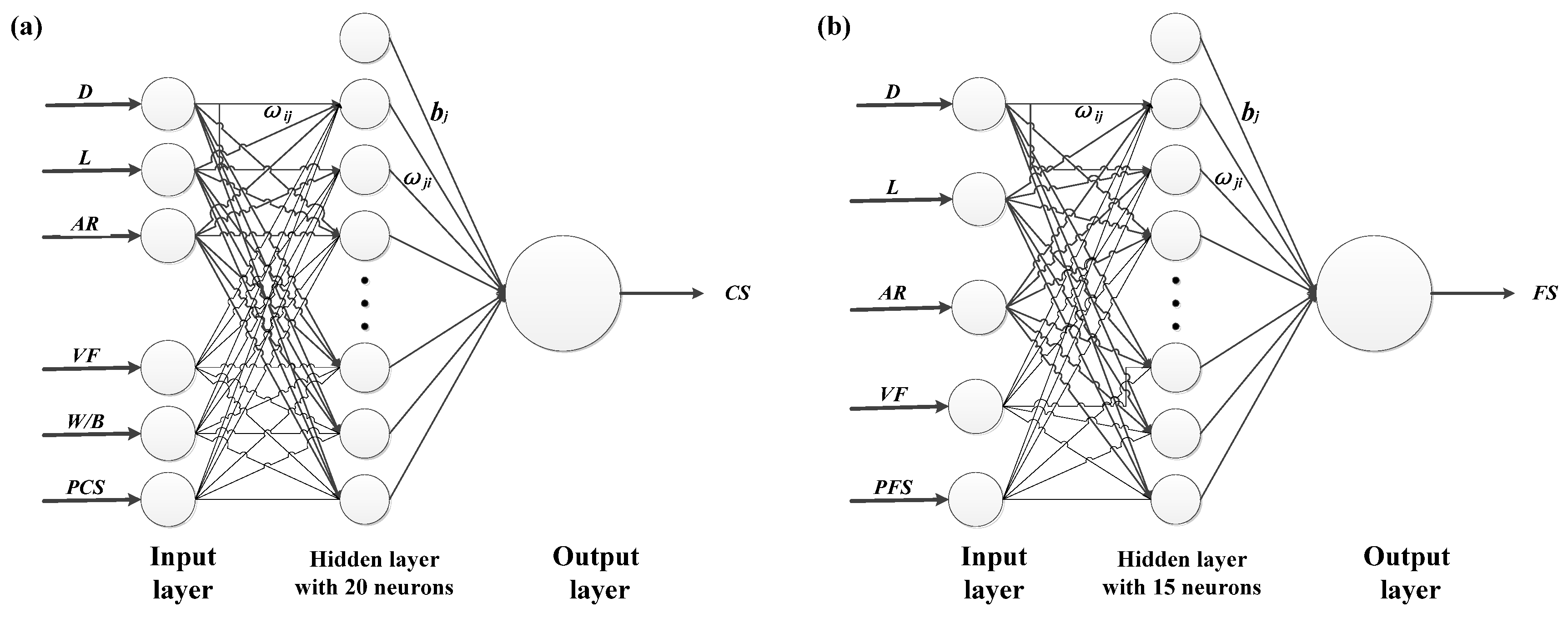
3.2. Proposed ANN Model
3.3. Processing Data
4. Results and Discussion
4.1. Results Assessment Criteria
4.2. Results Evaluation
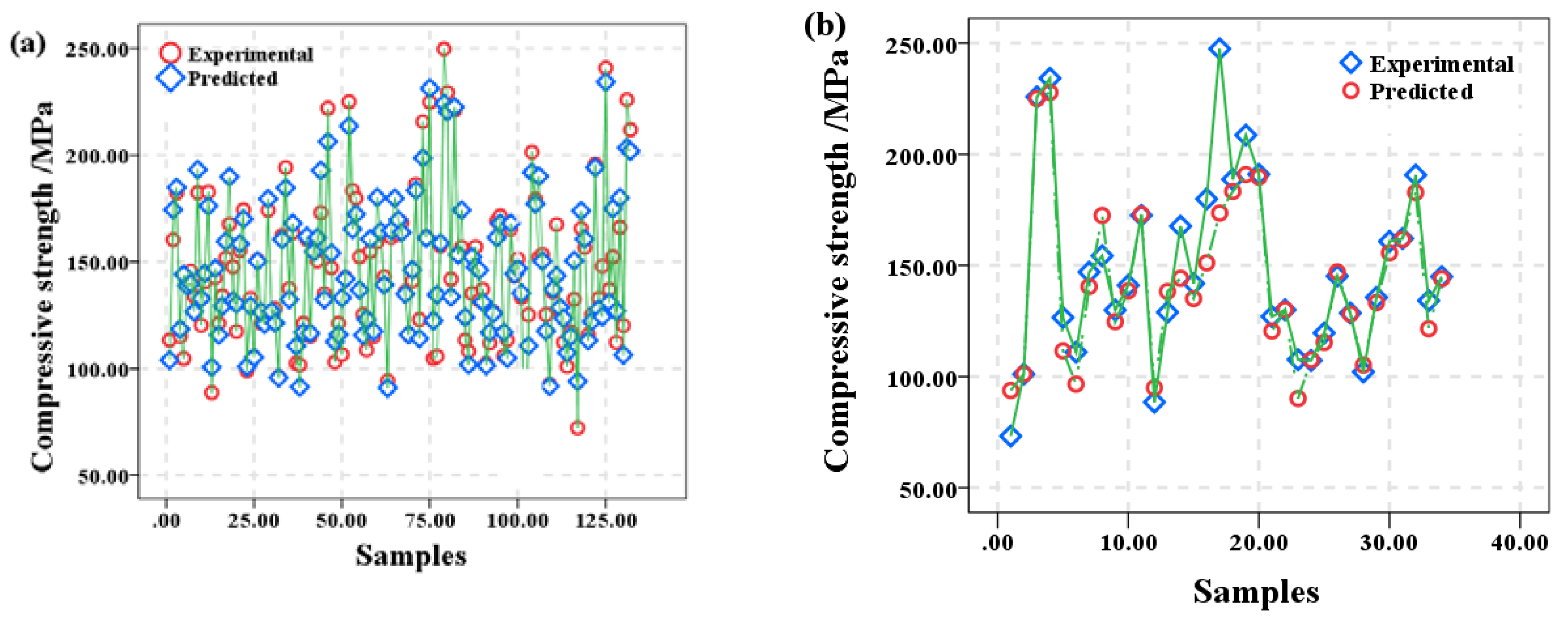
4.2.1. Predicting Model for Compressive Strength
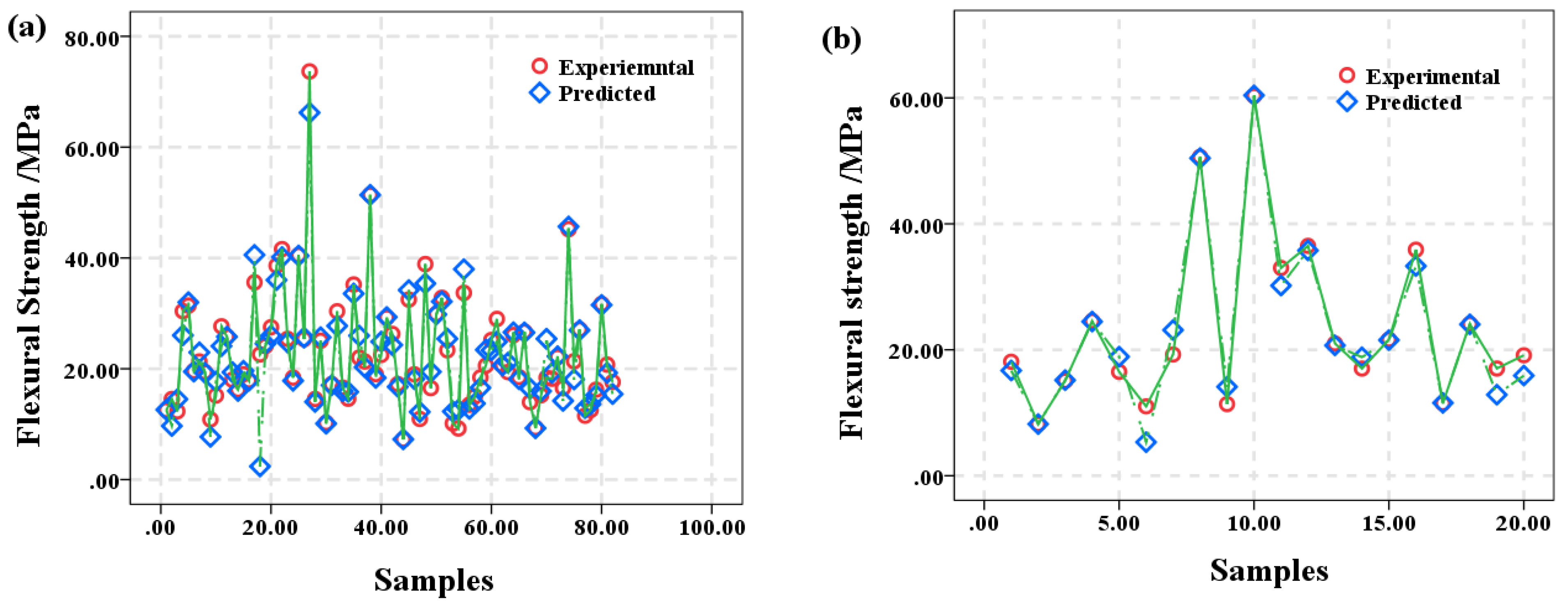
4.2.2. Prediction Model for Flexural Strength
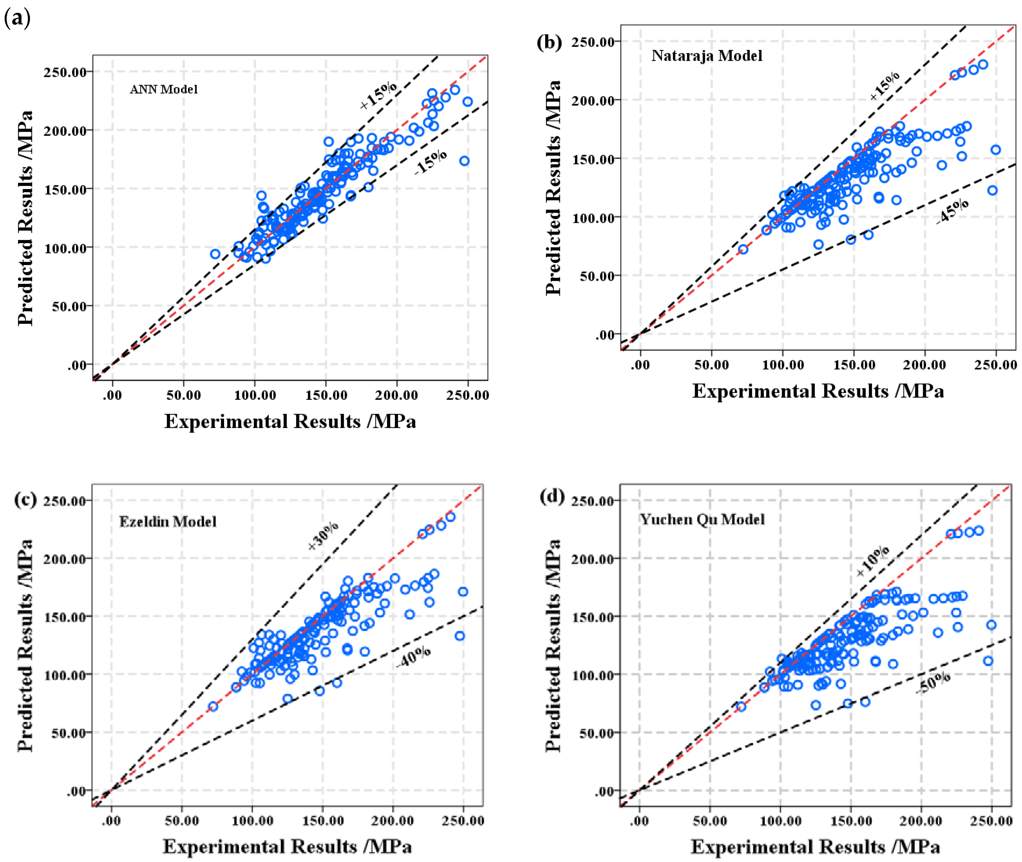
4.3. Comparison with Other Models
4.3.1. Compressive Strength Models
4.3.2. Flexural Strength Models
5. Conclusions
- (1)
- The compressive strength ANN model was trained by using the LM algorithm, with twenty neurons in hidden layers, revealing great prediction performance. The predicted values were fairly close to the experimental results for both the training and testing data sets in the proposed model.
- (2)
- The flexural strength ANN model was trained by using the LM algorithm, with twenty neurons in hidden layers, revealing great prediction performance. The predicted values were fairly close to the experimental results for both the training and testing data sets in the proposed model.
- (3)
- The results that were obtained from the compressive strength ANN model were compared with three analytical models proposed in other studies. The comparison indicated that the analytical models proposed by others may underestimate the compressive strength by approximately 10% on average, whereas the predicted values from the ANN model in this study agree with the experimental values.
- (4)
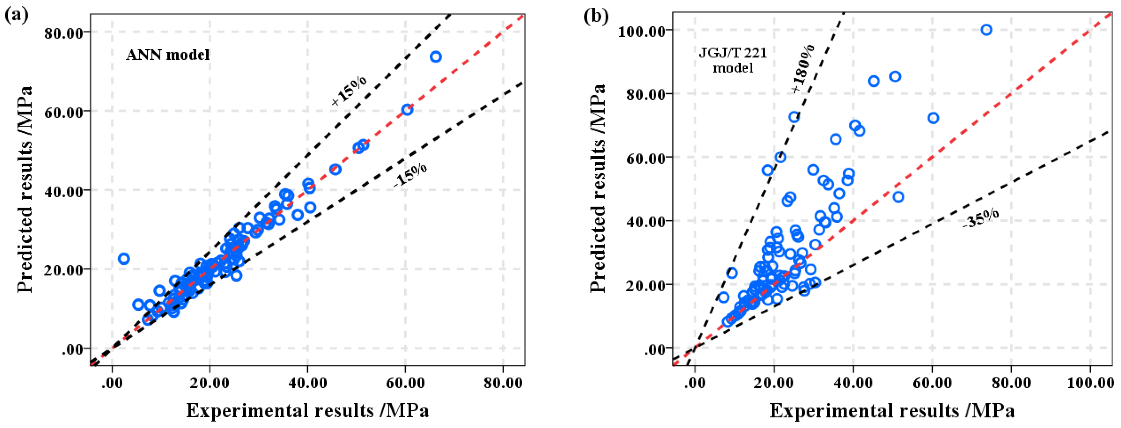
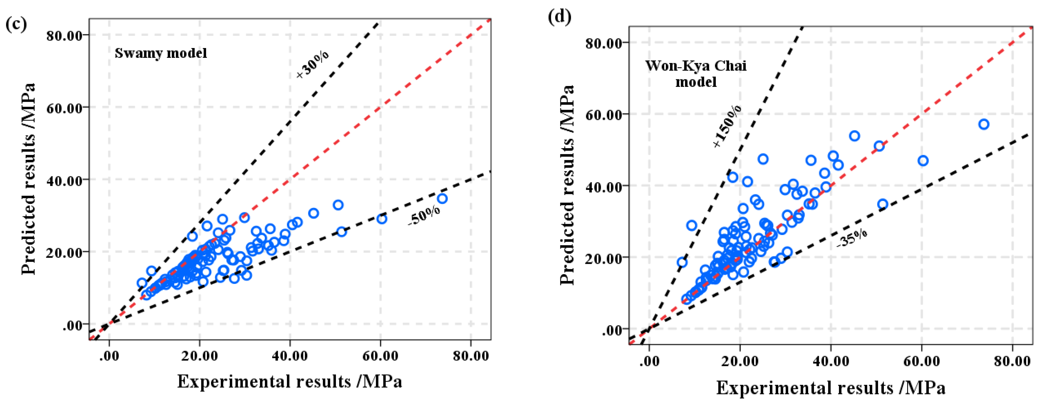
- The results obtained from the flexural strength ANN model were compared with three analytical models that were proposed in other studies. The comparison indicated that the analytical models proposed by others may varied from 0.8429 to 1.1458 on average values, whereas the predicted values from the ANN model in this study agree with the experimental values.
- (5)
- The ANN models that were proposed in this study have high applicability and reliability with respect to evaluating the effects of steel fibers on the compressive strength and the flexural strength of UHPFRC.
6. Research Limitations
Author Contributions
Funding
Conflicts of Interest
References
- Zdeb, T. An analysis of the steam curing and autoclaving process parameters for reactive powder concretes. Construct. Build. Mater. 2017, 131, 758–766. [Google Scholar] [CrossRef]
- Grünewald, S. Performance-Based Design of Self-Compacting Fiber Reinforced Concrete; Delft University of Technology: Delft, The Netherlands, 2004. [Google Scholar]
- Yu, R.; Spiesz, P.; Brouwers, H.J.H. Mix design and properties assessment of Ultra-High Performance Fiber Reinforced Concrete. Cem. Concr. Res. 2014, 56, 29–39. [Google Scholar] [CrossRef]
- Zhao, L.P.; Gao, D.Y.; Zhu, H.T. Effects of steel fibers on the strength and the ductility of concrete. J. North Chin. Inst. Water Conserv. Hydroelectr. Power 2012, 33, 29–32. [Google Scholar]
- Ortega, J.M.; Sánchez, I.; Climent, M.A. Impedance spectroscopy study of the effect of environmental conditions in the microstructure development of OPC and slag cement mortars. Materials 2017, 10, 569–583. [Google Scholar] [CrossRef]
- Sánchez, I. Influence of environment on durability of fly ash cement mortars. ACI Mater. J. 2012, 109, 647–656. [Google Scholar]
- Joshaghani, A.; Balapour, M.; Ramezanianpour, A.A. Effects of controlled environmental conditions on mechanical, microstructural and durability properties of cement mortar. Construct. Build. Mater. 2018, 164, 134–149. [Google Scholar] [CrossRef]
- Ramezanianpour, A.A.; Malhotra, V.M. Effects of curing on the compressive strength resistance to chloride-ion penetration and porosity of concrete incorporating slag, fly ash or silica fume. Cem. Concr. Compos. 1995, 17, 125–133. [Google Scholar] [CrossRef]
- Bae, B.; Choi, H.K.; Choi, C.S. Correlation between tensile strength and compressive strength of ultra-high strength concrete reinforced with steel fiber. J. Korea Concr. Inst. 2015, 27, 253–263. [Google Scholar] [CrossRef]
- Prem, P.R.; Bharatkumar, B.H.; Murthy, A.R. Influence of curing regime and steel fibers on the mechanical properties of UHPC. Mag. Concr. Res. 2015, 67, 988–1002. [Google Scholar] [CrossRef]
- Ayira, O.J.F. Investigating the properties of reactive powder concrete (RPC) compressive and flexural strength. Diss. Bachelor Eng. 2013, 4, 9758–9762. [Google Scholar]
- Khalil, W.; Damha, L.S. Mechanical properties of reactive powder concrete with various steel fiber and silica fume contents. ACTA Tecnia Corviniensis Bull. Eng. 2014, 7, 47–58. [Google Scholar]
- Guo, J. Influence of compressive strength of reactive powder concrete with different fibers. Concrete 2016, 5, 87–90. [Google Scholar]
- Ma, K.; Que, A.; Liu, C. Impact analysis of fibers on mechanical properties of reactive powder concrete. Concrete 2016, 3, 76–83. [Google Scholar]
- Zhong, S.; Wang, Y.; Gao, H. Effect of fibers on strength of self-compacting reactive powder concrete. J. Build. Mater. 2008, 11, 522–527. [Google Scholar]
- Wang, Q.; Guo, Z.; Xiang, Z.; Shao, J. Experimental research on proportion of reactive powder concrete 200 (RPC200). J. Arch. Civil Eng. Depart. 2007, 1, 70–74. [Google Scholar]
- Huang, L.; Xing, F.; Deng, L.; Huang, P. Study on factors affecting the strength of reactive powder concrete. J. Shenzhen Univ. Sci. Eng. 2004, 21, 178–182. [Google Scholar]
- Bi, Q.; Yang, Z.; Jiao, Q.; Wang, H. Experiment study on mechanical properties of a hubrid fiber reinforced reactive powder concrete. J. DaLian Jiaotong Univ. 2009, 30, 19–21. [Google Scholar]
- Zhang, P.; Kang, Q.; Shen, Z.; Wang, Z. Experimental research on the mechanical properties of steel fiber and carbon fiber reinforce RPC. Funct. Mater. 2010, 233–235. [Google Scholar]
- Wang, X.; Wang, Y. Mechanical properties of RPC with different steel fiber volume contents. J. Build. Mater. 2015, 18, 941–945. [Google Scholar]
- Wang, J.; Hao, X.; Ji, F. Effects of steel fibers on the mechanical properties of reactive powder concrete. Low Temp. Arch. Technol. 2018, 3, 18–20. [Google Scholar]
- Jia, F.; AN, M.; Zhang, H.; Yu, Z. Effect of fibers on bond properties between steel bar and reactive powder concrete. J. Build. Mater. 2012, 15, 847–851. [Google Scholar]
- Zhang, Q.; Wei, Y.; Zhang, J.; Feng, P. Influence of steel fiber content on fracture properties of RPC. J. Build. Mater. 2014, 17, 24–29. [Google Scholar]
- Zeng, J.; Wu, Y.; Lin, Q. Researches on the compressive mechanics properties of steel fiber RPC. J. Fuzhou Univ. Nat. Sci. 2005, 33, 132–137. [Google Scholar]
- Cao, X.; Peng, J.; LI, W. Study on mechanics properties of reactive powder concrete with different fibers. Chin. Concr. Cem. Product. 2014, 10, 54–57. [Google Scholar]
- Guo, T.; Teng, T.; Yu, Q. Influence of steel fibers contents on the strength and ductility of RPC. City House 2016, 23, 119–121. [Google Scholar]
- Jia, F.; Wang, W.; He, K.; Xia, Y.; Wang, J.; Zha, Y.; Kong, D. Study on basic properties of reactive powder concrete with different fiber. Chin. Concr. Cem. Product. 2016, 9, 53–56. [Google Scholar]
- Wang, Z.; Wang, J.; Yuan, J. Study on the Aggregates and mix Proportion of RPC. In Proceedings of the 13th National Academic Conference on Concrete and Prestressed Concrete, Beijing, China, 1 January 2016; pp. 342–347. [Google Scholar]
- Al-Tikrite, A.; Hadi, M.N.S. Mechanical properties of reactive powder concrete containing industrial and waste steel fibers at different ratios under compression. Construct. Build. Mater. 2017, 154, 1024–1034. [Google Scholar] [CrossRef]
- Maroliya, M.K. An investigation on reactive powder concrete containing steel fiber and fly ash. Int. J. Eng. Technol. Adv. Eng. 2012, 2, 538–545. [Google Scholar]
- Ministry of Housing and Urban-Rural Development of the People’s Republic of China (MOHURD). JGJ/T 221-2010: Technical Specification for Application of Fiber Reinforced Concrete; China Ministry of Construction, China Architecture & Building Press: Beijing, China, 2002.
- Swamy, R.N.; Mangat, P.S. A theory for the flexural strength of steel fiber reinforced concrete. Cem. Concr. Res. 1974, 4, 313–325. [Google Scholar] [CrossRef]
- Choi, W.K. An experimental study on the flexural strength of fiber reinforced concrete structure. Int. J. Saf. 2012, 11, 26–28. [Google Scholar]
- Nataraja, M.C.; Dhang, N.; Gupda, A.P. Stress-strain curves for steel fiber reinforced concrete under compression. Cem. Concr. Compos. 1999, 21, 383–390. [Google Scholar] [CrossRef]
- Ezeldin, A.S.; Balaguru, P.N. Normal and high strength fiber reinforced concrete under compression. J. Mater. Civil Eng. 1992, 4, 415–429. [Google Scholar] [CrossRef]
- Ou, Y.C.; Tsai, M.S.; Liu, K.; Chang, K.C. Compressive behavior of steel fiber-reinforced concrete with a high index. J. Mater. Civil Eng. 2012, 24, 207–215. [Google Scholar] [CrossRef]
- Nehdi, M.L.; Soliman, A.M. Artificial intelligence model for early-age autogenous shrinkage of concrete. ACI Mater. J. 2012, 109, 353–362. [Google Scholar]
- Cascardi, A.; Micelli, F.; Aiello, M.A. An artificial neural networks model for the prediction of the compressive strength of FRP-confined concrete circular columns. Eng. Struct. 2017, 140, 199–208. [Google Scholar] [CrossRef]
- Açikgenç, M.; Ulaş, M.; Alyamaç, K.E. Using an Artificial Neural Network to Predict Mix Compositions of Steel Fiber-Reinforced Concrete. Arab. J. Sci. Eng. 2015, 40, 407–419. [Google Scholar] [CrossRef]
- Vidivelli, B.; Jayaranjini, A. Prediction of compressive strength of high performance concrete containing industrial by products using artificial neural networks. Int. J. Civil Eng. Technol. 2016, 7, 302–314. [Google Scholar]
- Altun, F.; Kişi, Ö.; Aydin, K. Predicting the compressive strength of steel fiber added lightweight concrete using neural network. Comput. Mater. Sci. 2008, 42, 259–265. [Google Scholar] [CrossRef]
- Zealakshmi, D.; Ravichandran, A.; Kothandaraman, S. Prediction of Flexural Performance of Confined Hybrid Fibre Reinforced High Strength Concrete Beam by Artificial Neural Networks. Ind. J. Sci. Technol. 2016, 9, 1–6. [Google Scholar] [CrossRef]
- Sobhani, J.; Najimi, M.; Pourkhorshidi, A.; Parhizkar, T. Prediction of the compressive strength of no-slump concrete: A comparative study of regression, neural network and ANFIS models. Construct. Build. Mater. 2010, 24, 709–718. [Google Scholar] [CrossRef]
- Golafshani, E.M.; Rahai, A.; Sebt, M.H.; Akbarpour, H. Prediction of bond strength of spliced steel bars in concrete using artificial neural network and fuzzy logic. Construct. Build. Mater. 2012, 36, 411–418. [Google Scholar] [CrossRef]
- Sarıdemir, M. Predicting the compressive strength of mortars containing metakaolin by artificial neural networks and fuzzy logic. Adv. Eng. Softw. 2009, 40, 920–927. [Google Scholar] [CrossRef]
- Alshihri, M.M.; Azmy, A.M.; El-Bisy, M.S. Neural networks for predicting compressive strength of structural light weight concrete. Construct. Build. Mater. 2009, 23, 2214–2219. [Google Scholar] [CrossRef]
- China Standardization Administration. GB/T 31387-2015: Code for Reactive Powder Concrete, China Standardization Administration; China Architecture and Building Press: Beijing, China, 2015.
- Mansur, M.; Islam, M. Interpretation of concrete strength for nonstandard specimens. J. Mater. Civil Eng. 2002, 14, 151–155. [Google Scholar] [CrossRef]
- Lu, X.; Wang, Y.; Fu, C.; Zheng, W. Basic mechanical properties indexes of reactive powder concrete. J. Harbin Inst. Techanol. 2014, 46, 1–10. [Google Scholar]
- Benjamin, G.; Marshall, D. Cylinder or sube: Strengtrhtesting of 80 to 200 MPa (11.6 to 29 ksi) ultra-high-performance fiber-reinforced concrete. J. ACI Mater. 2008, 105, 603–609. [Google Scholar]
- Kusumawardaningsih, Y.; Fehling, E.; Ismail, M. UHPC compressive strength test specimens: Cylinder or cube. Procedia Eng. 2015, 125, 1076–1080. [Google Scholar] [CrossRef]


| No. | Specimen Dimension | * W/B | Steel Fiber | * PCS | ** CS | Reference | |||
|---|---|---|---|---|---|---|---|---|---|
| * D/mm | * L/mm | * AR | * VF/% | ||||||
| 1 | Cylinder D × H 100 mm × 200 mm | 0.30 | 0.20 | 13.00 | 65.00 | 0.00 | 94.17 | 94.17 | [9] |
| 2 | 0.30 | 0.20 | 13.00 | 65.00 | 0.50 | 94.17 | 96.13 | [9] | |
| 3 | 0.30 | 0.20 | 13.00 | 65.00 | 1.00 | 94.17 | 98.90 | [9] | |
| 4 | 0.30 | 0.20 | 13.00 | 65.00 | 2.00 | 94.17 | 103.05 | [9] | |
| 5 | 0.25 | 0.20 | 13.00 | 65.00 | 0.00 | 103.05 | 120.17 | [9] | |
| 6 | 0.25 | 0.20 | 13.00 | 65.00 | 0.50 | 103.05 | 122.90 | [9] | |
| 7 | 0.25 | 0.20 | 13.00 | 65.00 | 1.00 | 103.05 | 127.80 | [9] | |
| 8 | 0.25 | 0.20 | 13.00 | 65.00 | 2.00 | 103.05 | 133.19 | [9] | |
| 9 | 0.20 | 0.20 | 13.00 | 65.00 | 0.00 | 168.27 | 168.27 | [9] | |
| 10 | 0.20 | 0.20 | 13.00 | 65.00 | 0.50 | 168.27 | 174.27 | [9] | |
| 11 | 0.20 | 0.20 | 13.00 | 65.00 | 1.00 | 168.27 | 179.28 | [9] | |
| 12 | 0.20 | 0.20 | 13.00 | 65.00 | 2.00 | 168.27 | 182.31 | [9] | |
| 13 | 0.17 | 0.20 | 13.00 | 65.00 | 0.00 | 220.98 | 220.98 | [9] | |
| 14 | 0.17 | 0.20 | 13.00 | 65.00 | 0.50 | 220.98 | 225.83 | [9] | |
| 15 | 0.17 | 0.20 | 13.00 | 65.00 | 1.00 | 220.98 | 234.15 | [9] | |
| 16 | 0.17 | 0.20 | 13.00 | 65.00 | 2.00 | 220.98 | 240.75 | [9] | |
| 17 | Cube 70.7 mm × 70.7 mm × 70.7 mm | 0.16 | 0.16 | 13.00 | 81.25 | 2.50 | 126.59 | 172.59 | [10] |
| 18 | 0.16 | 0.16 | 13.00 | 81.25 | 2.00 | 126.59 | 163.31 | [10] | |
| 19 | 0.16 | 0.16 | 13.00 | 81.25 | 0.00 | 126.59 | 126.59 | [10] | |
| 20 | 0.16 | 0.16 | 6.00 | 37.50 | 2.50 | 126.59 | 171.37 | [10] | |
| 21 | 0.16 | 0.16 | 6.00 | 37.50 | 2.00 | 126.59 | 157.28 | [10] | |
| 22 | 0.16 | 0.16 | 6.00 | 37.50 | 0.00 | 126.59 | 126.59 | [10] | |
| 23 | Cube 100 mm × 100 mm × 100 mm | 0.24 | 0.20 | 20.00 | 100.00 | 0.00 | 111.00 | 111.00 | [11] |
| 24 | 0.24 | 0.20 | 20.00 | 100.00 | 1.00 | 111.00 | 101.00 | [11] | |
| 25 | 0.24 | 0.20 | 20.00 | 100.00 | 2.00 | 111.00 | 112.00 | [11] | |
| 26 | Cylinder D × H 100 mm × 200 mm | 0.14 | 0.50 | 30.00 | 60.00 | 0.00 | 141.72 | 141.72 | [12] |
| 27 | 0.14 | 0.50 | 30.00 | 60.00 | 1.00 | 141.72 | 146.99 | [12] | |
| 28 | 0.14 | 0.50 | 30.00 | 60.00 | 2.00 | 141.72 | 153.57 | [12] | |
| 29 | 0.15 | 0.50 | 30.00 | 60.00 | 3.00 | 141.72 | 154.33 | [12] | |
| 30 | Cube 100 mm × 100 mm × 100 mm | 0.18 | 0.24 | 13.5 | 56.25 | 0.00 | 129.92 | 129.92 | [13] |
| 31 | 0.18 | 0.24 | 13.5 | 56.25 | 1.00 | 129.92 | 135.89 | [13] | |
| 32 | 0.18 | 0.24 | 13.5 | 56.25 | 2.00 | 129.92 | 142.46 | [13] | |
| 33 | 0.18 | 0.24 | 13.5 | 56.25 | 3.00 | 129.92 | 155.09 | [13] | |
| 34 | 0.18 | 0.24 | 13.5 | 56.25 | 0.00 | 133.88 | 133.88 | [13] | |
| 35 | 0.18 | 0.24 | 13.5 | 56.25 | 1.00 | 133.88 | 141.06 | [13] | |
| 36 | 0.18 | 0.24 | 13.5 | 56.25 | 2.00 | 133.88 | 150.62 | [13] | |
| 37 | 0.18 | 0.24 | 13.5 | 56.25 | 3.00 | 133.88 | 160.43 | [13] | |
| 38 | 0.18 | 0.24 | 13.5 | 56.25 | 0.00 | 142.38 | 142.38 | [13] | |
| 39 | 0.18 | 0.24 | 13.5 | 56.25 | 1.00 | 142.38 | 153.25 | [13] | |
| 40 | 0.18 | 0.24 | 13.5 | 56.25 | 2.00 | 142.38 | 169.01 | [13] | |
| 41 | 0.18 | 0.24 | 13.5 | 56.25 | 3.00 | 142.38 | 172.52 | [13] | |
| 42 | Cube 70.7 mm × 70.7 mm × 70.7 mm | 0.20 | 0.20 | 13.00 | 65.00 | 0.00 | 88.49 | 88.49 | [14] |
| 43 | 0.20 | 0.20 | 13.00 | 65.00 | 0.50 | 88.49 | 105.37 | [14] | |
| 44 | 0.20 | 0.20 | 13.00 | 65.00 | 1.50 | 88.49 | 112.29 | [14] | |
| 45 | 0.20 | 0.20 | 13.00 | 65.00 | 2.50 | 88.49 | 128.91 | [14] | |
| 46 | 0.20 | 0.20 | 13.00 | 65.00 | 3.50 | 88.49 | 132.32 | [14] | |
| 47 | Prism 40 mm × 40 mm × 160 mm | 0.24 | 0.25 | 13.00 | 52.00 | 0.00 | 115.86 | 115.86 | [15] |
| 48 | 0.24 | 0.25 | 13.00 | 52.00 | 1.00 | 115.86 | 125.15 | [15] | |
| 49 | 0.24 | 0.25 | 13.00 | 52.00 | 1.50 | 115.86 | 126.40 | [15] | |
| 50 | 0.24 | 0.25 | 13.00 | 52.00 | 2.00 | 115.86 | 132.69 | [15] | |
| 51 | 0.24 | 0.25 | 13.00 | 52.00 | 2.50 | 115.86 | 137.32 | [15] | |
| 52 | Cube 100 mm × 100 mm × 100 mm | 0.23 | 0.20 | 13.00 | 65.00 | 2.00 | 145.55 | 161.30 | [16] |
| 53 | 0.23 | 0.20 | 13.00 | 65.00 | 4.00 | 145.55 | 186.30 | [16] | |
| 54 | 0.23 | 0.20 | 13.00 | 65.00 | 5.00 | 145.55 | 201.30 | [16] | |
| 55 | 0.23 | 0.20 | 13.00 | 65.00 | 0.00 | 145.55 | 145.55 | [16] | |
| 56 | Cube 70.7 mm × 70.7 mm × 70.7 mm | 0.20 | 0.22 | 13.00 | 59.09 | 0.00 | 72.15 | 72.15 | [17] |
| 57 | 0.20 | 0.22 | 13.00 | 59.09 | 1.00 | 72.15 | 125.10 | [17] | |
| 58 | 0.20 | 0.22 | 13.00 | 59.09 | 2.00 | 72.15 | 147.86 | [17] | |
| 59 | 0.20 | 0.22 | 13.00 | 59.09 | 3.00 | 72.15 | 160.17 | [17] | |
| 60 | Prism 40 mm × 40 mm × 160 mm | 0.25 | 0.24 | 13.00 | 54.17 | 0.00 | 108.04 | 108.04 | [18] |
| 61 | 0.16 | 0.24 | 13.00 | 54.17 | 0.50 | 108.04 | 113.39 | [18] | |
| 62 | 0.16 | 0.24 | 13.00 | 54.17 | 1.00 | 108.04 | 117.40 | [18] | |
| 63 | 0.16 | 0.24 | 13.00 | 54.17 | 1.50 | 108.04 | 135.66 | [18] | |
| 64 | 0.16 | 0.24 | 13.00 | 54.17 | 2.00 | 108.04 | 167.67 | [18] | |
| 65 | Prism 40 mm × 40 mm × 160 mm | 0.17 | 0.16 | 9.00 | 56.25 | 0.00 | 147.54 | 147.54 | [19] |
| 66 | 0.19 | 0.16 | 9.00 | 56.25 | 1.10 | 147.54 | 156.62 | [19] | |
| 67 | 0.19 | 0.16 | 9.00 | 56.25 | 2.10 | 147.54 | 194.07 | [19] | |
| 68 | 0.19 | 0.16 | 9.00 | 56.25 | 4.20 | 147.54 | 224.71 | [19] | |
| 69 | Cylinder D × H 50 mm × 100 mm | 0.19 | 0.22 | 13.00 | 59.09 | 0.00 | 105.92 | 105.92 | [20] |
| 70 | 0.19 | 0.22 | 13.00 | 59.09 | 1.00 | 105.92 | 141.86 | [20] | |
| 71 | 0.19 | 0.22 | 13.00 | 59.09 | 2.00 | 105.92 | 179.88 | [20] | |
| 72 | 0.19 | 0.22 | 13.00 | 59.09 | 4.00 | 105.92 | 247.41 | [20] | |
| 73 | Prism 40 mm × 40 mm × 160 mm | 0.20 | 0.22 | 13.00 | 59.09 | 0.00 | 162.86 | 162.86 | [21] |
| 74 | 0.20 | 0.22 | 13.00 | 59.09 | 0.50 | 162.86 | 182.61 | [21] | |
| 75 | 0.20 | 0.22 | 13.00 | 59.09 | 1.00 | 162.86 | 188.70 | [21] | |
| 76 | 0.20 | 0.22 | 13.00 | 59.09 | 1.50 | 162.86 | 208.61 | [21] | |
| 77 | 0.20 | 0.22 | 13.00 | 59.09 | 2.00 | 162.86 | 215.58 | [21] | |
| 78 | 0.20 | 0.22 | 13.00 | 59.09 | 2.50 | 162.86 | 221.88 | [21] | |
| 79 | 0.20 | 0.22 | 13.00 | 59.09 | 3.00 | 162.86 | 224.94 | [21] | |
| 80 | 0.20 | 0.22 | 13.00 | 59.09 | 3.50 | 162.86 | 229.25 | [21] | |
| 81 | 0.20 | 0.65 | 25.00 | 38.46 | 0.00 | 162.86 | 162.86 | [21] | |
| 82 | 0.20 | 0.65 | 25.00 | 38.46 | 1.50 | 162.86 | 174.08 | [21] | |
| 83 | 0.20 | 0.65 | 25.00 | 38.46 | 2.00 | 162.86 | 182.15 | [21] | |
| 84 | 0.20 | 0.65 | 25.00 | 38.46 | 2.50 | 162.86 | 190.97 | [21] | |
| 85 | 0.20 | 0.65 | 25.00 | 38.46 | 3.00 | 162.86 | 195.61 | [21] | |
| 86 | Cube 100 mm × 100 mm × 100 mm | 0.17 | 0.22 | 14.00 | 63.64 | 0.00 | 88.68 | 88.68 | [22] |
| 87 | 0.17 | 0.22 | 14.00 | 63.64 | 0.50 | 88.68 | 102.52 | [22] | |
| 88 | 0.17 | 0.22 | 14.00 | 63.64 | 1.00 | 88.68 | 127.00 | [22] | |
| 89 | 0.17 | 0.22 | 14.00 | 63.64 | 1.50 | 88.68 | 130.02 | [22] | |
| 90 | 0.17 | 0.22 | 14.00 | 63.64 | 2.00 | 88.68 | 142.87 | [22] | |
| 91 | Cube 100 mm × 100 mm × 100 mm | 0.17 | 0.15 | 13.00 | 86.67 | 0.00 | 107.60 | 107.60 | [23] |
| 92 | 0.17 | 0.15 | 13.00 | 86.67 | 1.00 | 107.60 | 125.20 | [23] | |
| 93 | 0.17 | 0.15 | 13.00 | 86.67 | 2.00 | 107.60 | 140.90 | [23] | |
| 94 | 0.17 | 0.15 | 13.00 | 86.67 | 0.00 | 107.60 | 131.80 | [23] | |
| 95 | 0.17 | 0.15 | 13.00 | 86.67 | 1.00 | 107.60 | 179.70 | [23] | |
| 96 | 0.17 | 0.15 | 13.00 | 86.67 | 2.00 | 107.60 | 211.80 | [23] | |
| 97 | Prism 100 mm × 100 mm × 400 mm | 0.22 | 0.23 | 13.00 | 57.78 | 0.00 | 107.23 | 107.23 | [24] |
| 98 | 0.22 | 0.23 | 13.00 | 57.78 | 0.50 | 107.23 | 119.58 | [24] | |
| 99 | 0.22 | 0.23 | 13.00 | 57.78 | 1.00 | 107.23 | 104.78 | [24] | |
| 100 | 0.22 | 0.23 | 13.00 | 57.78 | 2.00 | 107.23 | 105.74 | [24] | |
| 101 | 0.22 | 0.23 | 13.00 | 57.78 | 3.00 | 107.23 | 104.68 | [24] | |
| 102 | 0.22 | 0.23 | 13.00 | 57.78 | 0.00 | 147.10 | 147.10 | [24] | |
| 103 | 0.22 | 0.23 | 13.00 | 57.78 | 0.50 | 147.10 | 161.57 | [24] | |
| 104 | 0.22 | 0.23 | 13.00 | 57.78 | 1.00 | 147.10 | 163.59 | [24] | |
| 105 | 0.22 | 0.23 | 13.00 | 57.78 | 2.00 | 147.10 | 159.21 | [24] | |
| 106 | 0.22 | 0.23 | 13.00 | 57.78 | 3.00 | 147.10 | 151.94 | [24] | |
| 107 | 0.22 | 0.23 | 13.00 | 57.78 | 0.00 | 160.52 | 160.52 | [24] | |
| 108 | 0.22 | 0.23 | 13.00 | 57.78 | 1.00 | 160.52 | 165.13 | [24] | |
| 109 | 0.22 | 0.23 | 13.00 | 57.78 | 2.00 | 160.52 | 166.03 | [24] | |
| 110 | 0.22 | 0.23 | 13.00 | 57.78 | 3.00 | 160.52 | 167.99 | [24] | |
| 111 | Prism 100 mm × 100 mm × 400 mm | 0.16 | 0.22 | 13.50 | 61.36 | 0.00 | 125.80 | 125.80 | [25] |
| 112 | 0.16 | 0.22 | 13.50 | 61.36 | 2.00 | 125.80 | 145.20 | [25] | |
| 113 | 0.16 | 0.22 | 13.50 | 61.36 | 3.00 | 125.80 | 150.30 | [25] | |
| 114 | 0.16 | 0.22 | 13.50 | 61.36 | 4.00 | 125.80 | 152.20 | [25] | |
| 115 | 0.16 | 0.22 | 13.50 | 61.36 | 0.00 | 128.60 | 128.60 | [25] | |
| 116 | 0.16 | 0.22 | 13.50 | 61.36 | 2.00 | 128.60 | 151.20 | [25] | |
| 117 | 0.16 | 0.22 | 13.50 | 61.36 | 3.00 | 128.60 | 154.70 | [25] | |
| 118 | 0.16 | 0.22 | 13.50 | 61.36 | 4.00 | 128.60 | 156.80 | [25] | |
| 119 | 0.16 | 0.22 | 13.50 | 61.36 | 0.00 | 134.90 | 134.90 | [25] | |
| 120 | 0.16 | 0.22 | 13.50 | 61.36 | 2.00 | 134.90 | 156.90 | [25] | |
| 121 | 0.16 | 0.22 | 13.50 | 61.36 | 3.00 | 134.90 | 162.30 | [25] | |
| 122 | 0.16 | 0.22 | 13.50 | 61.36 | 4.00 | 134.90 | 165.50 | [25] | |
| 123 | Cube 100 mm × 100 mm × 100 mm | 0.20 | 0.25 | 14.00 | 56.00 | 0.00 | 101.70 | 101.70 | [26] |
| 124 | 0.20 | 0.25 | 14.00 | 56.00 | 1.00 | 101.70 | 113.40 | [26] | |
| 125 | 0.20 | 0.25 | 14.00 | 56.00 | 2.00 | 101.70 | 125.20 | [26] | |
| 126 | 0.20 | 0.25 | 14.00 | 56.00 | 3.50 | 101.70 | 133.60 | [26] | |
| 127 | 0.20 | 0.25 | 14.00 | 56.00 | 5.00 | 101.70 | 120.30 | [26] | |
| 128 | 0.20 | 0.25 | 14.00 | 56.00 | 0.00 | 92.50 | 92.50 | [26] | |
| 129 | 0.20 | 0.25 | 14.00 | 56.00 | 1.00 | 92.50 | 102.10 | [26] | |
| 130 | 0.20 | 0.25 | 14.00 | 56.00 | 2.00 | 92.50 | 115.80 | [26] | |
| 131 | 0.20 | 0.25 | 14.00 | 56.00 | 3.50 | 92.50 | 112.30 | [26] | |
| 132 | 0.20 | 0.25 | 14.00 | 56.00 | 5.00 | 92.50 | 106.60 | [26] | |
| 133 | 0.20 | 0.25 | 14.00 | 56.00 | 0.00 | 113.40 | 113.40 | [26] | |
| 134 | 0.20 | 0.25 | 14.00 | 56.00 | 1.00 | 113.40 | 121.20 | [26] | |
| 135 | 0.20 | 0.25 | 14.00 | 56.00 | 2.00 | 113.40 | 132.70 | [26] | |
| 136 | 0.20 | 0.25 | 14.00 | 56.00 | 3.50 | 113.40 | 144.30 | [26] | |
| 137 | 0.20 | 0.25 | 14.00 | 56.00 | 5.00 | 113.40 | 140.50 | [26] | |
| 138 | 0.20 | 0.25 | 14.00 | 56.00 | 0.00 | 124.09 | 124.90 | [26] | |
| 139 | 0.20 | 0.25 | 14.00 | 56.00 | 1.00 | 124.09 | 135.60 | [26] | |
| 140 | 0.20 | 0.25 | 14.00 | 56.00 | 2.00 | 124.09 | 143.20 | [26] | |
| 141 | 0.20 | 0.25 | 14.00 | 56.00 | 3.50 | 124.09 | 160.80 | [26] | |
| 142 | 0.20 | 0.25 | 14.00 | 56.00 | 5.00 | 124.09 | 162.10 | [26] | |
| 143 | Cube 100 mm × 100 mm × 100 mm | 0.14 | 0.22 | 13.00 | 59.09 | 0.00 | 108.72 | 108.72 | [27] |
| 144 | 0.14 | 0.22 | 13.00 | 59.09 | 0.50 | 108.72 | 121.36 | [27] | |
| 145 | 0.14 | 0.22 | 13.00 | 59.09 | 1.00 | 108.72 | 136.97 | [27] | |
| 146 | 0.14 | 0.22 | 13.00 | 59.09 | 1.50 | 108.72 | 152.19 | [27] | |
| 147 | 0.14 | 0.22 | 13.00 | 59.09 | 2.00 | 108.72 | 167.37 | [27] | |
| 148 | Prism 40 mm × 40 mm × 160 mm | 0.16 | 0.19 | 15.00 | 79.00 | 0.00 | 135.04 | 135.05 | [28] |
| 149 | 0.16 | 0.19 | 15.00 | 79.00 | 1.00 | 135.04 | 183.29 | [28] | |
| 150 | 0.16 | 0.19 | 15.00 | 79.00 | 2.00 | 135.04 | 190.67 | [28] | |
| 151 | 0.16 | 0.19 | 15.00 | 79.00 | 3.00 | 135.04 | 225.85 | [28] | |
| 152 | 0.16 | 0.19 | 15.00 | 79.00 | 4.00 | 135.04 | 249.68 | [28] | |
| 153 | Cylinder D × H 100 mm × 200 mm | 0.13 | 0.20 | 6.00 | 30.00 | 0.00 | 115.13 | 115.13 | [29] |
| 154 | 0.13 | 0.20 | 6.00 | 30.00 | 1.00 | 115.13 | 134.16 | [29] | |
| 155 | 0.13 | 0.20 | 6.00 | 30.00 | 2.00 | 115.13 | 136.95 | [29] | |
| 156 | 0.13 | 0.20 | 6.00 | 30.00 | 3.00 | 115.13 | 144.94 | [29] | |
| 157 | 0.13 | 0.20 | 6.00 | 30.00 | 4.00 | 115.13 | 151.64 | [29] | |
| 158 | 0.13 | 0.55 | 18.00 | 32.73 | 0.00 | 115.13 | 115.13 | [29] | |
| 159 | 0.13 | 0.55 | 18.00 | 32.73 | 1.00 | 115.13 | 121.22 | [29] | |
| 160 | 0.13 | 0.55 | 18.00 | 32.73 | 2.00 | 115.13 | 117.29 | [29] | |
| 161 | 0.13 | 0.55 | 18.00 | 32.73 | 3.00 | 115.13 | 121.22 | [29] | |
| 162 | 0.13 | 0.55 | 18.00 | 32.73 | 4.00 | 115.13 | 115.03 | [29] | |
| No. | Specimens Dimension | W/B | Steel Fiber | * PFS | ** FS | Reference | |||
|---|---|---|---|---|---|---|---|---|---|
| D/mm | L/mm | AR | VF/% | ||||||
| 1 | Prism 40 mm × 40 mm × 160 mm | 0.15 | 0.40 | 13.00 | 32.50 | 0.00 | 18.00 | 18.00 | [30] |
| 2 | 0.17 | 0.40 | 13.00 | 32.50 | 0.20 | 18.00 | 27.50 | [30] | |
| 3 | 0.18 | 0.40 | 13.00 | 32.50 | 0.20 | 18.00 | 22.00 | [30] | |
| 4 | 0.15 | 0.40 | 13.00 | 32.50 | 0.00 | 19.00 | 19.00 | [30] | |
| 5 | 0.17 | 0.40 | 13.00 | 32.50 | 0.20 | 19.00 | 29.00 | [30] | |
| 6 | 0.18 | 0.40 | 13.00 | 32.50 | 0.20 | 19.00 | 22.50 | [30] | |
| 7 | Prism 40 mm × 40 mm × 160 mm | 0.30 | 0.20 | 13.00 | 65.00 | 0.00 | 10.95 | 10.95 | [9] |
| 8 | 0.30 | 0.20 | 13.00 | 65.00 | 0.50 | 10.95 | 12.54 | [9] | |
| 9 | 0.30 | 0.20 | 13.00 | 65.00 | 1.00 | 10.95 | 14.55 | [9] | |
| 10 | 0.30 | 0.20 | 13.00 | 65.00 | 2.00 | 10.95 | 16.23 | [9] | |
| 11 | 0.25 | 0.20 | 13.00 | 65.00 | 0.00 | 11.54 | 11.54 | [9] | |
| 12 | 0.25 | 0.20 | 13.00 | 65.00 | 0.50 | 11.54 | 13.51 | [9] | |
| 13 | 0.25 | 0.20 | 13.00 | 65.00 | 1.00 | 11.54 | 15.02 | [9] | |
| 14 | 0.25 | 0.20 | 13.00 | 65.00 | 2.00 | 11.54 | 16.51 | [9] | |
| 15 | 0.20 | 0.20 | 13.00 | 65.00 | 0.00 | 13.97 | 13.97 | [9] | |
| 16 | 0.20 | 0.20 | 13.00 | 65.00 | 0.50 | 13.97 | 15.24 | [9] | |
| 17 | 0.20 | 0.20 | 13.00 | 65.00 | 1.00 | 13.97 | 17.24 | [9] | |
| 18 | 0.20 | 0.20 | 13.00 | 65.00 | 2.00 | 13.97 | 18.40 | [9] | |
| 19 | 0.17 | 0.20 | 13.00 | 65.00 | 0.00 | 15.11 | 18.43 | [9] | |
| 20 | 0.17 | 0.20 | 13.00 | 65.00 | 0.50 | 15.11 | 16.24 | [9] | |
| 21 | 0.17 | 0.20 | 13.00 | 65.00 | 1.00 | 15.11 | 18.11 | [9] | |
| 22 | 0.17 | 0.20 | 13.00 | 65.00 | 2.00 | 15.11 | 19.04 | [9] | |
| 23 | Prism 100 mm × 100 mm × 500 mm | 0.24 | 0.20 | 20.00 | 100.00 | 0.00 | 8.23 | 8.23 | [11] |
| 24 | 0.24 | 0.20 | 20.00 | 100.00 | 1.00 | 8.23 | 7.24 | [11] | |
| 25 | 0.24 | 0.20 | 20.00 | 100.00 | 2.00 | 8.23 | 9.34 | [11] | |
| 26 | Prism100 mm × 100 mm × 500 mm | 0.14 | 0.50 | 30.00 | 60.00 | 0.00 | 9.22 | 9.22 | [12] |
| 27 | 0.14 | 0.50 | 30.00 | 60.00 | 1.00 | 9.22 | 15.07 | [12] | |
| 28 | 0.14 | 0.50 | 30.00 | 60.00 | 2.00 | 9.22 | 24.57 | [12] | |
| 29 | 0.15 | 0.50 | 30.00 | 60.00 | 3.00 | 9.22 | 29.24 | [12] | |
| 30 | Prism100 mm × 100 mm × 400 mm | 0.20 | 0.20 | 13.00 | 65.00 | 0.00 | 10.13 | 10.13 | [14] |
| 31 | 0.20 | 0.20 | 13.00 | 65.00 | 0.50 | 10.13 | 12.55 | [14] | |
| 32 | 0.20 | 0.20 | 13.00 | 65.00 | 1.50 | 10.13 | 15.17 | [14] | |
| 33 | 0.20 | 0.20 | 13.00 | 65.00 | 2.50 | 10.13 | 16.51 | [14] | |
| 34 | 0.20 | 0.20 | 13.00 | 65.00 | 3.50 | 10.13 | 20.66 | [14] | |
| 35 | Prism 40 mm × 40 mm × 160 mm | 0.24 | 0.25 | 13.00 | 52.00 | 0.00 | 11.02 | 11.02 | [15] |
| 36 | 0.24 | 0.25 | 13.00 | 52.00 | 1.00 | 11.02 | 12.33 | [15] | |
| 37 | 0.24 | 0.25 | 13.00 | 52.00 | 1.50 | 11.02 | 16.51 | [15] | |
| 38 | 0.24 | 0.25 | 13.00 | 52.00 | 2.00 | 11.02 | 19.25 | [15] | |
| 39 | 0.24 | 0.25 | 13.00 | 52.00 | 2.50 | 11.02 | 25.36 | [15] | |
| 40 | Prism 40 mm × 40 mm × 160 mm | 0.20 | 0.22 | 13.00 | 59.09 | 2.00 | 26.68 | 29.90 | [16] |
| 41 | 0.20 | 0.22 | 13.00 | 59.09 | 4.00 | 26.68 | 50.63 | [16] | |
| 42 | 0.20 | 0.22 | 13.00 | 59.09 | 5.00 | 26.68 | 73.67 | [16] | |
| 43 | 0.20 | 0.22 | 13.00 | 59.09 | 0.00 | 26.68 | 26.68 | [16] | |
| 44 | Prism 40 mm × 40 mm × 160 mm | 0.16 | 0.24 | 13.00 | 54.17 | 0.00 | 10.25 | 10.25 | [18] |
| 45 | 0.16 | 0.24 | 13.00 | 54.17 | 0.50 | 10.25 | 11.38 | [18] | |
| 46 | 0.16 | 0.24 | 13.00 | 54.17 | 1.00 | 10.25 | 20.75 | [18] | |
| 47 | 0.16 | 0.24 | 13.00 | 54.17 | 1.50 | 10.25 | 27.66 | [18] | |
| 48 | 0.16 | 0.24 | 13.00 | 54.17 | 2.00 | 10.25 | 30.38 | [18] | |
| 49 | Prism 40 mm × 40 mm × 160 mm | 0.17 | 0.16 | 9.00 | 56.25 | 0.00 | 22.60 | 22.60 | [19] |
| 50 | 0.19 | 0.16 | 9.00 | 56.25 | 1.10 | 22.60 | 25.80 | [19] | |
| 51 | 0.19 | 0.16 | 9.00 | 56.25 | 2.10 | 22.60 | 51.40 | [19] | |
| 52 | 0.19 | 0.16 | 9.00 | 56.25 | 4.20 | 22.60 | 60.30 | [19] | |
| 53 | Prism 40 mm × 40 mm × 160 mm | 0.20 | 0.22 | 13.00 | 59.09 | 0.00 | 16.60 | 16.60 | [21] |
| 54 | 0.20 | 0.22 | 13.00 | 59.09 | 0.50 | 16.60 | 17.24 | [21] | |
| 55 | 0.20 | 0.22 | 13.00 | 59.09 | 1.00 | 16.60 | 19.60 | [21] | |
| 56 | 0.20 | 0.22 | 13.00 | 59.09 | 1.50 | 16.60 | 21.30 | [21] | |
| 57 | 0.20 | 0.22 | 13.00 | 59.09 | 2.00 | 16.60 | 26.10 | [21] | |
| 58 | 0.20 | 0.22 | 13.00 | 59.09 | 2.50 | 16.60 | 33.00 | [21] | |
| 59 | 0.20 | 0.22 | 13.00 | 59.09 | 3.00 | 16.60 | 35.20 | [21] | |
| 60 | 0.20 | 0.22 | 13.00 | 59.09 | 3.50 | 16.60 | 36.50 | [21] | |
| 61 | 0.20 | 0.65 | 13.00 | 38.46 | 1.50 | 16.60 | 17.60 | [21] | |
| 62 | 0.20 | 0.65 | 13.00 | 38.46 | 2.00 | 16.60 | 18.50 | [21] | |
| 63 | 0.20 | 0.65 | 13.00 | 38.46 | 2.50 | 16.60 | 19.00 | [21] | |
| 64 | 0.20 | 0.65 | 13.00 | 38.46 | 3.00 | 16.60 | 21.00 | [21] | |
| 65 | Prism 100 mm × 100 mm × 400 mm | 0.16 | 0.22 | 13.50 | 61.36 | 0.00 | 17.02 | 17.02 | [25] |
| 66 | 0.16 | 0.22 | 13.50 | 61.36 | 2.00 | 17.02 | 20.58 | [25] | |
| 67 | 0.16 | 0.22 | 13.50 | 61.36 | 3.00 | 17.02 | 23.36 | [25] | |
| 68 | 0.16 | 0.22 | 13.50 | 61.36 | 4.00 | 17.02 | 18.38 | [25] | |
| 69 | 0.16 | 0.22 | 13.50 | 61.36 | 0.00 | 22.11 | 22.11 | [25] | |
| 70 | 0.16 | 0.22 | 13.50 | 61.36 | 2.00 | 22.11 | 24.10 | [25] | |
| 71 | 0.16 | 0.22 | 13.50 | 61.36 | 3.00 | 22.11 | 21.63 | [25] | |
| 72 | 0.16 | 0.22 | 13.50 | 61.36 | 4.00 | 22.11 | 25.06 | [25] | |
| 73 | Prism 100 mm × 100 mm × 400 mm | 0.20 | 0.25 | 14.00 | 56.00 | 0.00 | 14.60 | 14.60 | [26] |
| 74 | 0.20 | 0.25 | 14.00 | 56.00 | 1.00 | 14.60 | 19.40 | [26] | |
| 75 | 0.20 | 0.25 | 14.00 | 56.00 | 2.00 | 14.60 | 27.10 | [26] | |
| 76 | 0.20 | 0.25 | 14.00 | 56.00 | 3.50 | 14.60 | 35.90 | [26] | |
| 77 | 0.20 | 0.25 | 14.00 | 56.00 | 5.00 | 14.60 | 38.60 | [26] | |
| 78 | 0.20 | 0.25 | 14.00 | 56.00 | 0.00 | 11.50 | 11.50 | [26] | |
| 79 | 0.20 | 0.25 | 14.00 | 56.00 | 1.00 | 11.50 | 17.90 | [26] | |
| 80 | 0.20 | 0.25 | 14.00 | 56.00 | 2.00 | 11.50 | 25.20 | [26] | |
| 81 | 0.20 | 0.25 | 14.00 | 56.00 | 3.50 | 11.50 | 30.40 | [26] | |
| 82 | 0.20 | 0.25 | 14.00 | 56.00 | 5.00 | 11.50 | 31.70 | [26] | |
| 83 | 0.20 | 0.25 | 14.00 | 56.00 | 0.00 | 18.20 | 18.20 | [26] | |
| 84 | 0.20 | 0.25 | 14.00 | 56.00 | 1.00 | 18.20 | 26.30 | [26] | |
| 85 | 0.20 | 0.25 | 14.00 | 56.00 | 2.00 | 18.20 | 31.40 | [26] | |
| 86 | 0.20 | 0.25 | 14.00 | 56.00 | 3.50 | 18.20 | 33.70 | [26] | |
| 87 | 0.20 | 0.25 | 14.00 | 56.00 | 5.00 | 18.20 | 35.60 | [26] | |
| 88 | 0.20 | 0.25 | 14.00 | 56.00 | 0.00 | 19.40 | 19.40 | [26] | |
| 89 | 0.20 | 0.25 | 14.00 | 56.00 | 1.00 | 19.40 | 24.10 | [26] | |
| 90 | 0.20 | 0.25 | 14.00 | 56.00 | 2.00 | 19.40 | 32.80 | [26] | |
| 91 | 0.20 | 0.25 | 14.00 | 56.00 | 3.50 | 19.40 | 38.90 | [26] | |
| 92 | 0.20 | 0.25 | 14.00 | 56.00 | 5.00 | 19.40 | 40.50 | [26] | |
| 93 | Prism 100 mm × 100 mm × 400 mm | 0.14 | 0.22 | 13.00 | 59.09 | 0.00 | 10.85 | 10.85 | [27] |
| 94 | 0.14 | 0.22 | 13.00 | 59.09 | 0.50 | 10.85 | 14.54 | [27] | |
| 95 | 0.14 | 0.22 | 13.00 | 59.09 | 1.00 | 10.85 | 17.03 | [27] | |
| 96 | 0.14 | 0.22 | 13.00 | 59.09 | 1.50 | 10.85 | 19.13 | [27] | |
| 97 | 0.16 | 0.22 | 13.00 | 59.09 | 2.00 | 10.85 | 21.37 | [27] | |
| 98 | Prism 40 mm × 40 mm × 160 mm | 0.16 | 0.19 | 15.00 | 79.00 | 0.00 | 21.30 | 21.30 | [28] |
| 99 | 0.16 | 0.19 | 15.00 | 79.00 | 1.00 | 21.30 | 25.40 | [28] | |
| 100 | 0.16 | 0.19 | 15.00 | 79.00 | 2.00 | 21.30 | 32.50 | [28] | |
| 101 | 0.16 | 0.19 | 15.00 | 79.00 | 3.00 | 21.30 | 41.60 | [28] | |
| 102 | 0.16 | 0.19 | 15.00 | 79.00 | 4.00 | 21.30 | 45.20 | [28] | |
| Variables | Compressive Strength | Flexural Strength | ||
|---|---|---|---|---|
| Minimum | Maximum | Minimum | Maximum | |
| W/B | 0.13 | 0.30 | — | — |
| D/mm | 0.15 | 0.65 | 0.16 | 0.65 |
| L/mm | 6 | 30 | 9 | 30 |
| AR | 100 | 30 | 32.5 | 100 |
| VF/% | 0.00 | 5.00 | 0.00 | 5.00 |
| PCS/MPa | 72.15 | 220.98 | 8.23 | 26.88 |
| CS/MPa | 72.15 | 249.68 | 8.23 | 73.67 |
| Parameters | Flexural Strength Model | Compressive Strength Model |
|---|---|---|
| Number of input layer nodes | 5 | 6 |
| Number of hidden layers | 1 | 1 |
| Number of hidden layer nodes | 15 | 20 |
| Number of output layer nodes | 1 | 1 |
| Momentum factor | 0.8 | 0.6 |
| Learning rate | 0.3 | 0.3 |
| Target error | 0.00001 | 0.00001 |
| Learning cycle | 10,000 | 10,000 |
| Indicators | Training | Testing |
|---|---|---|
| RMS | 0.0876 | 0.0980 |
| R2 | 0.9923 | 0.9901 |
| IAE | 0.0005 | 0.0019 |
| Indicators | Training | Testing |
|---|---|---|
| RMS | 0.1492 | 0.0376 |
| R2 | 0.9777 | 0.9986 |
| IAE | 0.0011 | 0.0004 |
| Analytical Model | Compressive Strength |
|---|---|
| Nataraja [34] | |
| Ezeldin [35] | |
| Yuchen Qu [36] |
| Models | Mean | SD | IAE |
|---|---|---|---|
| ANN model | 1.0050 | 0.0896 | 0.70% |
| Nataraja model | 0.9152 | 0.1191 | 1.13% |
| Ezeldin model | 0.9454 | 0.1216 | 1.03% |
| Yuchen Qu model | 0.8830 | 0.1268 | 1.34% |
| Analytical Model | Flexural Strength |
|---|---|
| JGJ/T 221 [31] | |
| Swamy [32] | |
| Won-Kya Chai [33] |
| Models | Mean | SD | IAE |
|---|---|---|---|
| ANN model | 0.9915 | 0.1509 | 1.50% |
| JGJ/T 221 model | 1.2807 | 0.4431 | 4.04% |
| Swamy model | 0.8429 | 0.2055 | 3.03% |
| Won-Kya Chai model | 1.1458 | 0.3547 | 3.30% |
© 2018 by the authors. Licensee MDPI, Basel, Switzerland. This article is an open access article distributed under the terms and conditions of the Creative Commons Attribution (CC BY) license (http://creativecommons.org/licenses/by/4.0/).
Share and Cite
Qu, D.; Cai, X.; Chang, W. Evaluating the Effects of Steel Fibers on Mechanical Properties of Ultra-High Performance Concrete Using Artificial Neural Networks. Appl. Sci. 2018, 8, 1120. https://doi.org/10.3390/app8071120
Qu D, Cai X, Chang W. Evaluating the Effects of Steel Fibers on Mechanical Properties of Ultra-High Performance Concrete Using Artificial Neural Networks. Applied Sciences. 2018; 8(7):1120. https://doi.org/10.3390/app8071120
Chicago/Turabian StyleQu, Dechao, Xiaoping Cai, and Wei Chang. 2018. "Evaluating the Effects of Steel Fibers on Mechanical Properties of Ultra-High Performance Concrete Using Artificial Neural Networks" Applied Sciences 8, no. 7: 1120. https://doi.org/10.3390/app8071120
APA StyleQu, D., Cai, X., & Chang, W. (2018). Evaluating the Effects of Steel Fibers on Mechanical Properties of Ultra-High Performance Concrete Using Artificial Neural Networks. Applied Sciences, 8(7), 1120. https://doi.org/10.3390/app8071120