1. Introduction
The stator of a three-phase induction machine is a three-phase winding, where the rotor does not require a DC magnetic field circuit during operation; consequently, rotor currents are generated by the relative motion between the stator and rotor magnetic fields. From the interaction between stator and rotor magnetic fields, induction torque is generated in the motor [
1]. Since the architecture is simple and easy to operate, induction motors have become the most commonly used AC motor.
With the advancement of technology and the improvement of demand, precision control is the direction of inevitable efforts. For induction motors, their identities will not be provided solely by power, but will be promoted to the center of control. The control method and system design of the induction machine both require the equivalent model [
2], which can be divided into two kinds: steady state and dynamic. The acquisition of parameters is divided into off-line estimation and on-line estimation [
3].
A typical case of parameter estimation in off-line estimation is the IEEE standard 112 test, which uses the stator DC test, blocked rotor test, and no-load test to obtain the relevant parameters of the equivalent circuit [
4]. In the blocked rotor test, the separation of the stator reactance and the rotor reactance is generally based on empirical rules. The no-load test emphasizes the measurement of the rotation loss. Its estimated value is sufficient for a steady-state analysis to provide approximate parameters [
5]. In the differential evolution method, a broad range of each parameter was considered, and the convergence of the algorithm was satisfactory, attesting to the robustness of the method [
6]. The method fits the steady-state experimental data to the stator current locus for various slip frequencies in the stator flux linkage reference-frame [
7], and can better able estimate the core loss conductance. A method based on Artificial Neural Networks (ANN) and Adaptive Neuro-Fuzzy Inference Systems (ANFIS) has also been proposed [
8]. This method calculates the equivalent circuit parameters using the data from the manufacturer including torque, active and reactive power, starting current, maximum torque, full load speed, and efficiency. The use of variable frequency tests for the computation of the equivalent electrical circuit parameters has also been proposed [
9]. The sparse grid optimization algorithm is achieved by matching the response of the machine’s mathematical model with the recorded stator current and voltage signals. This approach is noninvasive as it uses external measurements, resulting in reduced system complexity and cost [
10]. An estimation method is carried out by recording the stator terminal voltage during natural braking and subsequent offline curve fitting. The algorithm allows for an accurate reconstruction of the mechanical time constant as well as loading torque speed dependency [
11].
Under normal circumstances, online estimations must include equipment and controllers. When the device is connected to the controller, there must be a set of procedures to adjust its internal parameters [
12,
13,
14]. In the presence of load, single-phase signals are often used for adjustment such as DC or AC signals. The DC signal can be used to adjust and determine the resistance, while the rest of the parameters must be determined by the response of the control excitation frequency [
15]. In addition, some scholars have considered the magnetization curve to estimate the parameters under rated operation [
16]. Constructing different operating points under different test conditions and using pulse-width modulation technology to control the excitation can also produce satisfactory results [
17]. Going further, the genetic algorithm has been applied to induction motor efficiency estimation by the DC test, voltages, currents, input power, and speed measurements [
18].
Several problems are encountered when solving the above parameters [
19,
20]; namely: (1) there are unavoidable noises in the actual signal that interfere with the calculation results; and (2) the actual system is far more complex than the model we are considering and will cause errors in the linearly derived system.
This paper proposes a polynomial fractional regression method. This method provides the ability to obtain the optimal value via only one calculation, without the requirement of any initial value and avoids any local optimal solution. The theoretical impedance-slip rate characteristic curve of the induction machine can be expressed as a polynomial fraction so that a proper polynomial fraction can obtain complete and accurate parameters. The minimum objective function of the polynomial fraction can be expressed as an equation of polynomial regression, which is without the initial value and iterative steps. This method has two advantages: first, as long as the calculation is done once, the optimum value can be obtained, eliminating a large number of iteration steps; and second, it does not need to provide the initial value, which avoids falling into the local minimum solution, thereby simplifying the computational complexity [
21,
22]. In an induction machine, the relationship between the impedance and the slip rate can be described in terms of polynomial fractions; consequently, the paper extends polynomial regression to the regression of polynomial fractions to improve its application.
To achieve the above purpose, the proposed method includes the following steps. First, it acquires the time-varying signals of voltage, current, and rotor speed when the induction machine is started. Second, it calculates the resistance and reactance of the induction machine under different slip rates. Third, it estimates the equivalent circuit parameters of the induction machine. Fourth, it simulates the dynamic behavior of the induction machine and calculate its output torque. Finally, it calculates the parameters of the equivalent mechanical model.
2. Theory
2.1. Impedance at Different Slip Rates
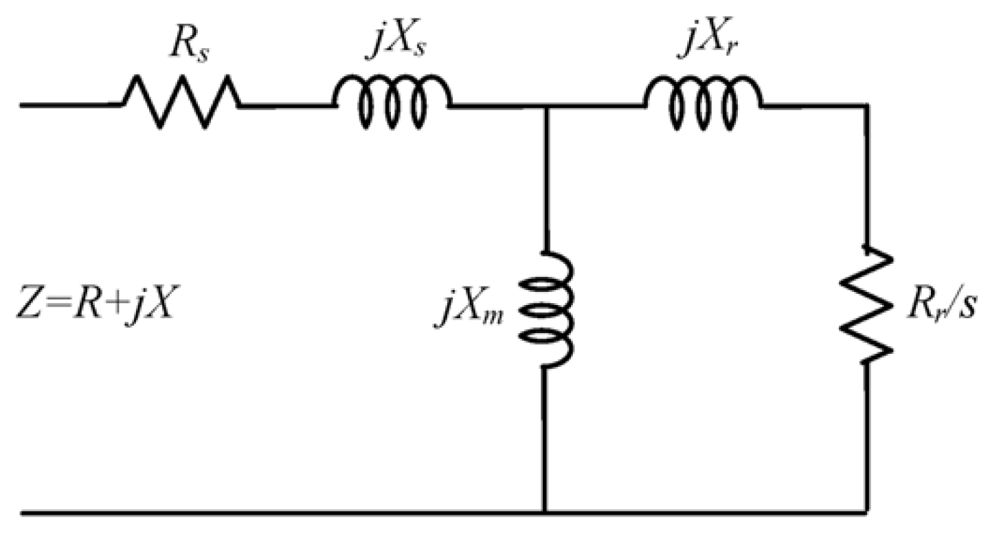
The most commonly used models in induction machine analysis can be divided into two categories: the transient model and the steady state model. As the transient time of the induction machine is very short, the transience caused by the inductor will quickly fall to the negligible range in the early stage of start-up, so the characteristics of voltage and current will be dominated by the steady-state impedance. The equivalent circuit of the induction machine under the steady state is shown in
Figure 1, where
Rs is the stator resistance;
Rr is the rotor resistance referred to the stator side;
Xm is the excitation reactance;
Xs is the stator equivalent reactance;
Xr is the rotor reactance referred to the stator side;
Z is the input impedance;
R is the input resistance;
X is the input reactance; and
s is the slip rate. The input impedance of the induction machine can be expressed as
Dividing the resistance and reactance in the impedance, the input resistance and input reactance are respectively:
In
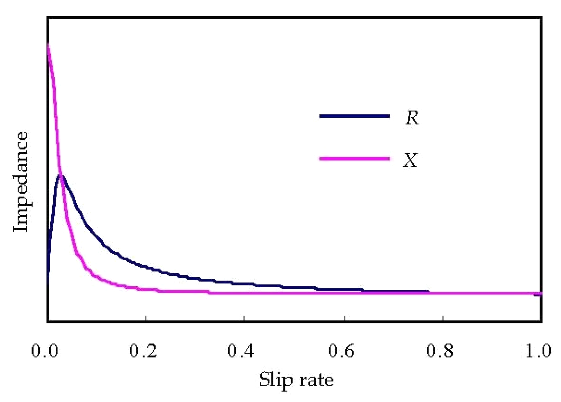
Figure 1, only the resistance is affected by the slip rate. Due to the change in the resistance, both the input resistance and the input reactance are affected and become time-varying impedance. When the rotor speed changes from a static to synchronous state, the slip rate changes from 1 to 0, and the resistance and reactance changes are shown in
Figure 2. The values of the curves will vary with the capacity, however, the trend of the curve will remain the same. Therefore, the vertical axis does not mark the scale. In
Figure 2, the reactance is a monotonically decreasing curve. At the beginning of the start-up, the reactance is flat and there is no change, but the resistance increases at the beginning of the start-up, with a maximum reading near the synchronous speed [
23]. The reactance value and the resistance value will intersect near the maximum resistance value, and when the slip rate continues to decrease, the resistance drops rapidly, so when the slip rate is zero, the resistance drops to nearly zero. Expressed in polynomial fractions, the input resistance and input reactance can be expressed as
Therefore, the input impedance can be expressed as a polynomial fraction.
Comparing Equations (4)–(6), the relationship between the polynomial fractional coefficients and the induction machine parameters is
2.2. Polynomial Fractional Regression
This paper used polynomial fractional regression to obtain the relevant parameters. The principle is to use polynomial fractions to represent the relationship between the variables and dependent variables. By minimizing the objective function, the set of results can be close to the actual value. When the induction machine is started, instantaneous values of voltage, current, and rotation speed can be obtained through the sensors. From these instantaneous values, a series of time-varying effective values can be obtained [
24]. A series of data,
n, can be obtained from the above experiment
where
N is the number of acquisitions.
Assume that the relation between the two variables is polynomial, as shown in Equation (6). The error between the experimental data and polynomial fraction,
En, is
To estimate the optimal solution of the polynomial, the objective function
EE can be set as
The minimum of
E, that can be found by each partial derivative of
EE, is 0, which satisfies the following conditions:
Therefore, the following equations can be obtained
It can be expressed in a matrix form:
where
The coefficients of the polynomial fraction can be found as
2.3. Equivalent Circuit Parameter Calculation
Although there are five variables and six equations in Equations (7)–(12), it does not mean that each parameter of the equivalent circuit can be obtained independently.
Xm,
Xr, and
Rr/
s form series/parallel circuits. The equivalent circuit is a series connection of resistor and reactance. The resistance is shown in Equation (2), where it can be seen that
Rs and
Rr are independent of each other and their solutions can be obtained separately. The reactance part is shown in Equation (3), and is equivalent to a fixed reactance and a reactance that changes with the slip rate due to the series/parallel circuit. The fixed reactance will be combined with the stator reactance as a complete reactance so that the three reactances cannot be obtained separately. This article set the distribution of reactance to a specific ratio
η, i.e.,
The general
η value was about 0.95 to 1.05. Introducing Equations (7)–(12) into
η values
The excitation reactance
Xm is
Rotor reactance referred to the stator side
Xr is
Rotor resistance referred to the stator side
Rr is
This article uses an optimized method to estimate
Rs as
2.4. Dynamic Simulation
This paper calculated the torque of the induction machine by dynamic simulation. The parameters of the equivalent circuit can be obtained by the aforementioned method. Under the stator reference architecture, the dynamic model can be expressed as [
25]
where
iqs and
ids are the d-q coordinates stator currents;
iqr and
idr are the d-q coordinates rotor currents;
vqs and
vds are the d-q coordinates stator voltages;
vqr and
vdr are the d-q coordinates rotor voltages;
Ls is stator inductance;
Lm is excitation inductance;
Lr is equivalent rotor inductance;
is rotor speed; and
p is the differentiation factor. Therefore, the output torque
Tout can be further obtained.
where
P is the number of poles.
2.5. Inertia and Friction Coefficient
Inertia and the friction coefficient determine the relationship between output torque and rotor speed. That is, when the output torque and rotor speed are known, inertia
J and friction coefficient
B can be further obtained. Assuming that the torque only causes the rotor speed to change, in time domain,
t, the relationship between rotor speed and torque conforms to the following differential equations:
In discrete data, this can be expressed as
When considering the inertia and friction coefficient is constant, to obtain the most appropriate parameters, set the objective function
ET as
When the objective function is the minimum, the most appropriate
J and
B are obtained, i.e., the gradients for Equation (44) are both zero, and thus
J and
B can be obtained by
2.6. Procedure
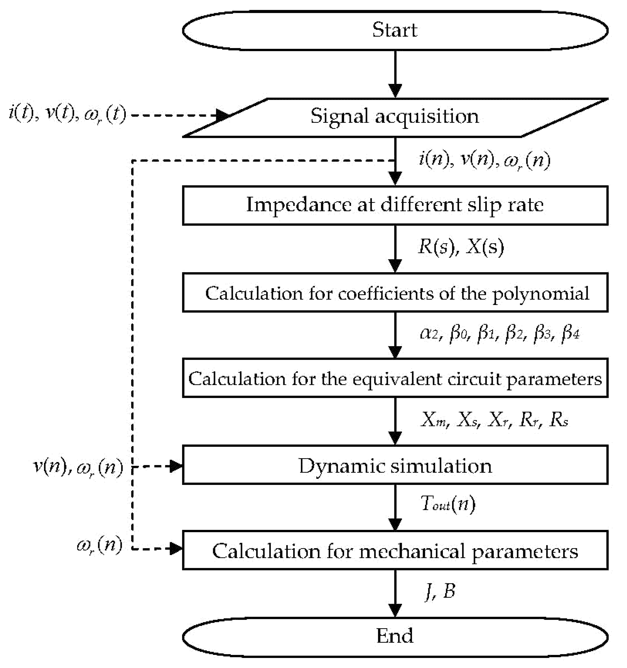
This section organizes the above theory as a complete procedure.
Figure 3 presents the flowchart, and the illustration shows the following:
Step 1, signal acquisition. Acquire the signals of the voltage, current, and rotor speed when the induction machine is started.
Step 2, impedance at different slip rate. According to Equation (13), calculate the input resistance and reactance values at different slip rates.
Step 3, calculation for coefficients of the polynomial fraction. According to Equation (29), the coefficients of the polynomial fraction can be obtained.
Step 4, calculation for the equivalent circuit parameters. Equivalent circuit parameters can be obtained from Equations (32)–(36).
Step 5, dynamic simulation. Based on the equivalent circuit parameters, input voltage, and the rotor speed, dynamic simulation of Equations (37)–(41) can be performed.
Step 6, calculation for mechanical parameters. Inertia and the friction coefficient can be obtained according to Equation (45).
Step 7, calculation completed.
3. Results and Discussion
The first section explains the estimation results of the polynomial fractions and verifies the reliability of the method. Following this, the analysis of a practical induction machine was used as an example to illustrate the application of this method. The second section estimates the parameters of the actual induction machine. The third section simulates the dynamic performance by the obtained parameters and compares it with the actual signal. The last section explains the results of the mechanical parameter analysis.
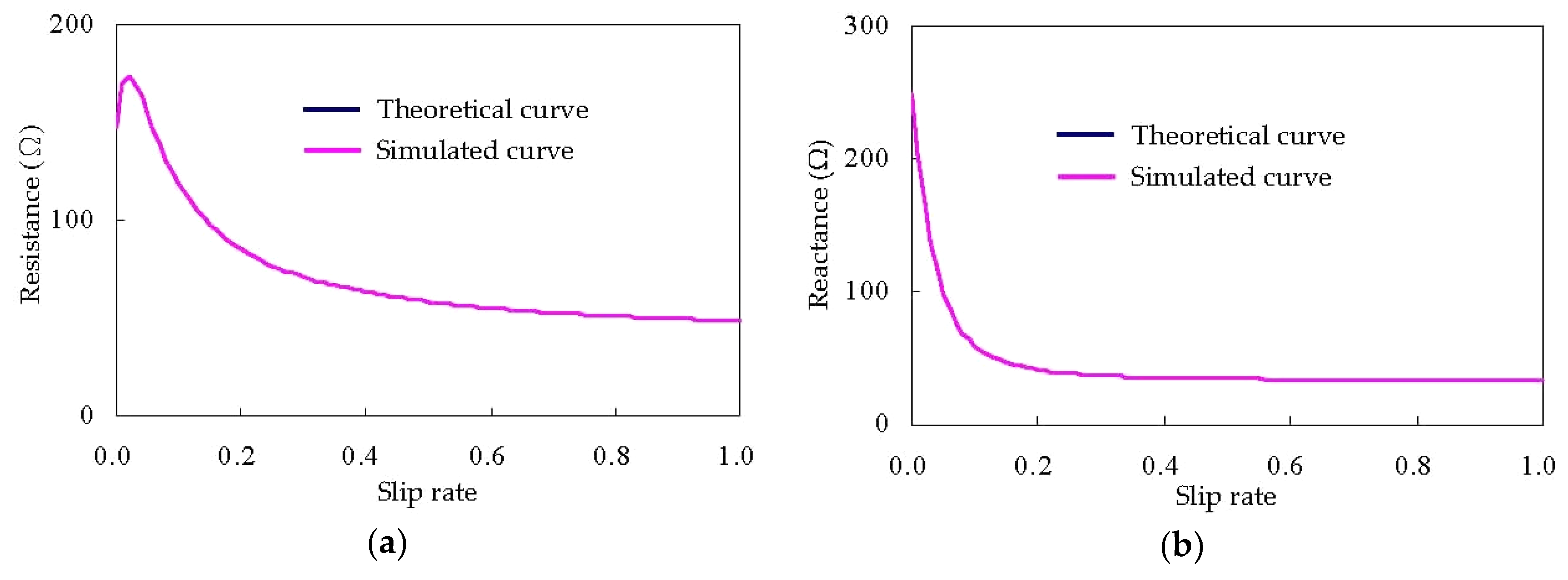
3.1. Theoretical Verification Analysis
This paper evaluated the analysis results of the polynomial fractions with theoretical values. The equivalent circuit of a three-phase induction machine is shown in
Figure 1. The parameters were set as
Rs = 38 Ω,
Rr = 12 Ω,
Xm = 288 Ω,
Xs = 17 Ω, and
Xr = 17 Ω. The slip-impedance characteristic curve was obtained as shown in
Figure 4. Using the polynomial fractional fitting of Equation (29), the parameters were obtained as per
Table 1. It was found that this method could obtain the optimal parameters of the equivalent circuit in one calculation. As the values of
Xm,
Xs, and
Xr depend on each other, this paper set their proportional relationship to
η. The significance of
η has already been described in Equation (30), but regardless of the value of
η, the slip-impedance characteristic curves obtained from these values are all in perfect agreement with the theoretical values, as shown in
Figure 4, demonstrating the reliability of this method.
3.2. Equivalent Circuit Parameters of Field Test
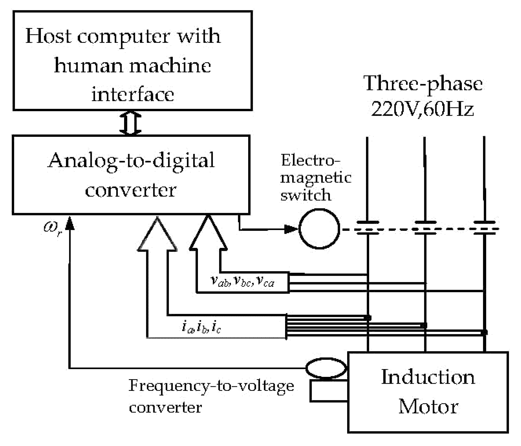
This paper built a practical set of equipment based on personal computers by using personal computers with peripheral equipment, data acquisition systems and data output modules and appropriate software programs to complete a real-time online monitoring system. The complete hardware architecture consisted of an induction machine, sensors, analog–to–digital converters, control circuitry, a computer, and setup as shown in
Figure 5. The induction machine was three-phase, four-pole, 1/2 HP, 60 Hz. The voltage and current signals were obtained from the voltage probe and the current transformer, respectively, and the rotor speed was obtained through the frequency–to–voltage converter, then converted into the deuterium signal by the analog–to–digital converter and stored in the computer. The analog–to–digital converter was a National Instruments 6036E data acquisition device. The sample rate was set at 1024 samples/s, with the number of samples set at 922 and a sample period of 0.9 s. The power control circuit was switched by an electromagnetic switch, while independent on/off control of the device could be performed on command. The host computer was used as a monitoring device using National Instruments LabVIEW as a human machine interface.
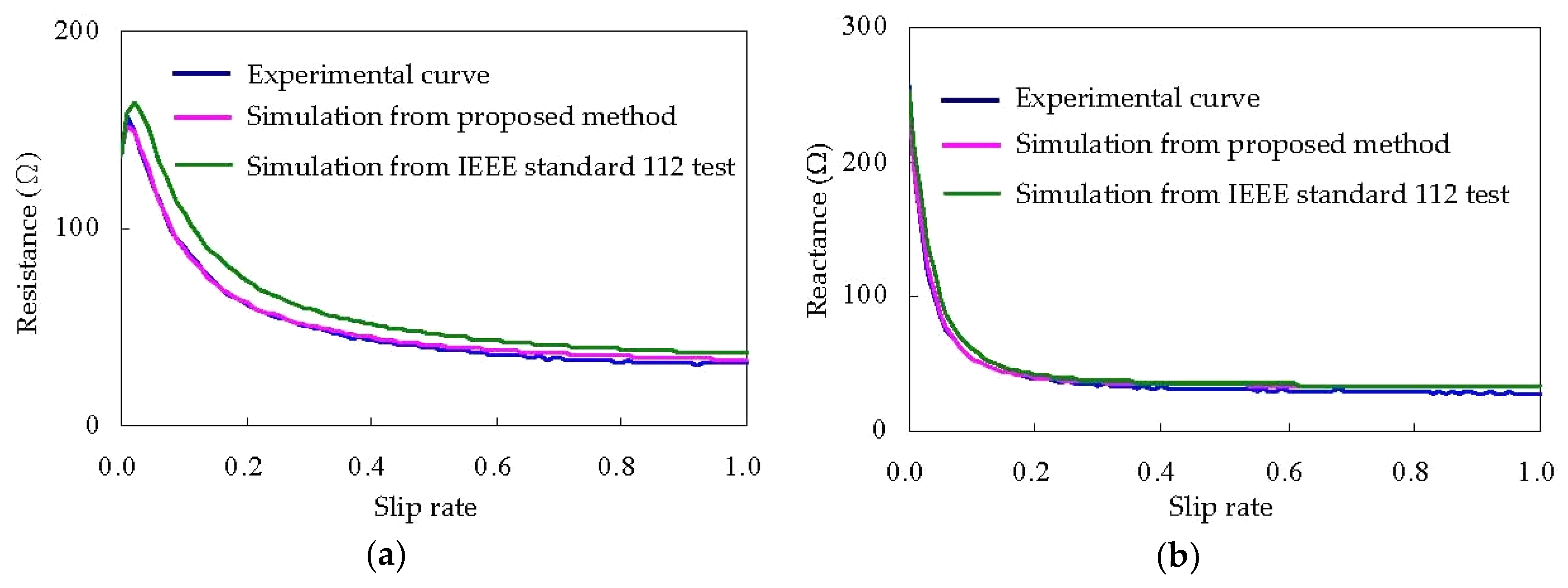
The simulated slip-impedance characteristic curve is shown in
Figure 6. It was found that these coefficients were very high-fitting to the experimental one and had quite satisfactory results. The simulated slip-impedance characteristic curve with induction machine parameters from IEEE 112 test is also shown in
Figure 6. Some obvious errors were found, which arose from unpredictable nonlinear components and other disturbances; however, this method still obtained the largest approximation.
Due to the saturation phenomenon in the induction machine, some of the parameters appeared nonlinear as the operating point changed. For the saturation phenomenon, generally speaking, the nonlinear inductance represents the magnetic saturation effect, and the inductance value at saturation is smaller than that at unsaturation, and under different currents, different inductance values are used. This will also complicate the equivalent circuit; however, since the estimated curve was very close to the actual curve in this example, magnetic saturation was not considered.
3.3. Dynamic Simulation
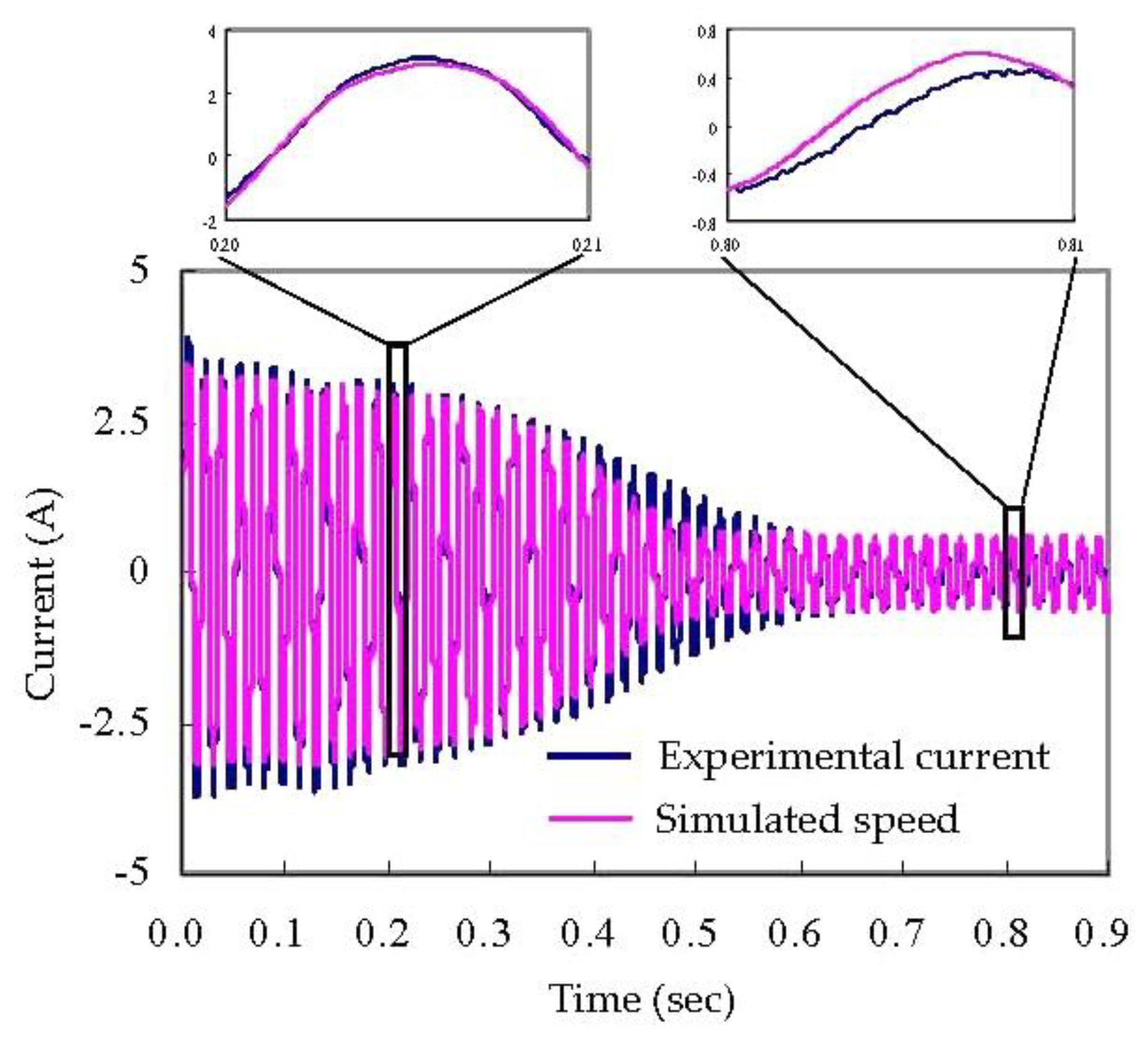
In this paper, the obtained parameters were used to simulate the dynamic behavior of the speed and compare it with the experimental values. The simulation result and the experimental one are shown in
Figure 7. It was found that the two were quite close. The current in
Figure 7 will show steady-state results, and confirms the steady-state term dominates the current variation.
3.4. Inertia and Friction Coefficient
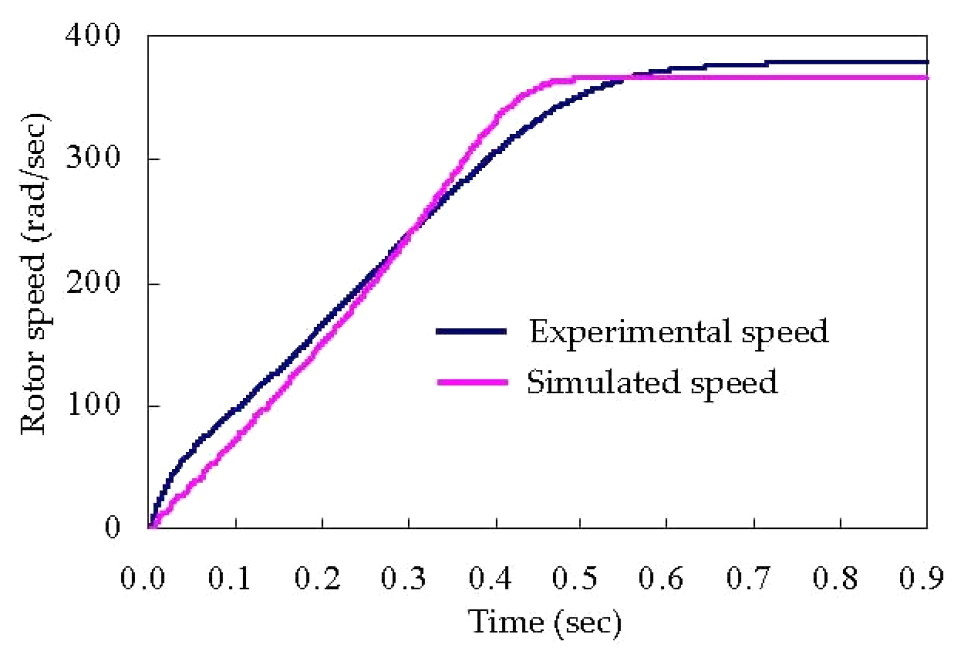
Figure 8 shows the comparison of the simulated speed and the experimental one. According to Equation (45), the inertia and friction coefficient of the induction machine were
J = 0.38 (g·m
2) and
B = 0.61 (mN·m/(rad/s)). This result also determined the objective function of Equation (44) as 8.388 (rad/s), which was a rather low value. It confirmed that the parameters obtained by this method were quite consistent with the actual situation.
However, it was found that the objective function of the mechanical system was larger than the objective function of the equivalent circuit. The reason was due to the non-linear relationship between the mechanical load and the rotor speed, where the well-known wind loss is the third power of the rotor speed. Therefore, fixing the operating conditions will inevitably result in errors.
In addition, errors occur in the steady state. The reason is that the polynomial fraction optimization optimizes the curve segment, and if the optimization result has a more accurate estimation in the transient state, there will be a less accurate estimation in the steady state; similarly, if the steady-state signal is increased, that of the transient will have poor estimation results.
This method uses polynomial fractions to calculate the curve parameters and will vary depending on the curve segment. It estimates the induction machine parameters in two stages: equivalent circuit parameters and mechanical system parameters. The equivalent circuit parameter estimation range was s = 0~1, and the analysis scope was clear, so a stable result could be obtained. The mechanical system parameter estimation range was t = 0~T, where T is the time of the sampling section, which will vary due to the length of the steady-state selection period, and different Ts will produce different parameters. As a result, the estimation of the mechanical system parameter changes greatly. This is a common problem faced by the estimation methods.
4. Conclusions
The proposed method is an off-line estimation, which uses the time-varying voltage, current, and rotor speed to calculate the parameters of an induction machine. In this paper, polynomial regression was used to calculate the steady-state equivalent circuit parameters. The output torque and the rotor speed can be used to estimate the inertia and the friction coefficient of the machine. The evaluation showed that this method was fully consistent with the analysis of theoretical values, and maintained a very high degree of fit in the analysis of real values, verifying the accuracy and reliability of the method. Through this method, the user can analyze the signal of the induction machine at one time and completely grasp the parameters of the induction machine.
This method was based on polynomials. The result of polynomial analysis will be affected by the sampling section, and different sections will have different results. This characteristic will not produce differences in the equivalent circuit parameter estimation, but will cause slight differences in the mechanical system parameter estimation.
In future studies, researchers might consider the representation and estimation of equivalent magnetic circuits for magnetic saturation phenomena. Non-linear loads might also significantly affect the accuracy of the parameters, so if more accurate results are needed, further modeling of non-linear loads is required.


