Article

HM3alD: Polymorphic Malware Detection Using Program Behavior-Aware Hidden Markov Model

Faculty of Electrical and Computer Engineering, Tarbiat Modares University, P.O. Box 14115-194 Tehran, Iran
*
Author to whom correspondence should be addressed.
Appl. Sci. 2018, 8(7), 1044; https://doi.org/10.3390/app8071044
Submission received: 24 May 2018 / Revised: 15 June 2018 / Accepted: 25 June 2018 / Published: 26 June 2018

Abstract

:
Malware have been tremendously growing in recent years. Most malware use obfuscation techniques for evasion and hiding purposes, but they preserve the functionality and malicious behavior of original code. Although most research work has been mainly focused on program static analysis, some recent contributions have used program behavior analysis to detect malware at run-time. Extracting the behavior of polymorphic malware is one of the major issues that affects the detection result. In this paper, we propose HM3alD, a novel program behavior-aware hidden Markov model for polymorphic malware detection. The main idea is to use an effective clustering scheme to partition the program behavior of malware instances and then apply a novel hidden Markov model (called program behavior-aware HMM) on each cluster to train the corresponding behavior. Low-level program behavior, OS-level system call sequence, is mapped to high-level action sequence and used as transition triggers across states in program behavior-aware HMM topology. Experimental results show that HM3alD outperforms all current dynamic and static malware detection methods, especially in term of FAR, while using a large dataset of 6349 malware.

1. Introduction

Endpoint security is regarded as the most important and the last defense point in security threats [1]. According to this requirement, malware detection is the vital issue in computer security. Today, malware are assumed as essential threats in the software industry [2]. In an annual report, Symantec mentions that just in 2015 alone more than 430 × 106 malware variants were created [3]. In this regard, many methods have been proposed that focus on detecting and classifying malware [1]. Due to the increasing growth of malware, anti-viruses are usually unable to completely detect them, because malware programs usually attempt to hide themselves using obfuscation methods so they are hard to detect by static analysis [4].

1.1. Malware

The terms malicious software and malware refer to any computer program that performs malicious activities on a host or accesses a private computer system to gather sensitive information from users without their knowledge. From the beginning of malware’s existence, they used code obfuscation to evade detection. Using the obfuscation technique, malware authors generate new malware variants of known malware and easily bypass detection methods. Polymorphism is another attribute that is commonly employed by malware. Polymorphism is an encryption technique that is used to mutate the static binary code of malware to prevent their detection [5]. When an infected program is run, the malware is decrypted and loaded into memory and then infects other programs and/or any type of executable content and tries to run a new version of itself [5]. These malware use a permutation engine to produce a new encryption procedure at runtime. If a malware presents a new behavior (by new functionalities or by combining the features of existing malware), it is called a zero day malware. Malware variants refer to all new malware that are produced manually or automatically from any existing malware [4,5].

1.2. Malware Analysis and Detection

Malware analysis is the process of understanding malware behavior and how to detect and eliminate them by capturing the important characteristics of a given malware sample [6]. This is particularly important for preventing and detecting future cyber attacks against the host and network. There are two main methods of analyzing malware, known as static and dynamic analyses. Static analysis (i.e., code analysis) examines the sample program without running it and inspects the program’s binary code to determine its behavior. Static analysis explores all possible execution paths in a program—not just those invoked during execution—but it cannot deal with malware employing anti-reverse engineering technologies such as code packing and obfuscation [6]. Dynamic analysis (i.e., behavior analysis) executes the program in a controlled environment and monitors its behavior. Thus, dynamic analysis explores what function with what arguments is called and detects most obfuscation attempts [6]. The combination of these two methods, hybrid method, could certainly further improve the detection results [7].
Based on malware analysis type, malware detection methods in general fall into two categories: signature-based and anomaly-based. Signature-based (i.e., knowledge or misuse) detection methods use some common sequence patterns (i.e., signatures found in the binary code of malware instances) to identify malware. Most often, signature-based detection methods are very fast because they do not run samples to identify malware. Note that this method is used on most popular commercial antivirus software. The main drawback of signature-based methods is that they are not effective against polymorphism and obfuscation methods, so they cannot detect modified and unknown malicious executables [8,9].
Anomaly-based detection methods build a reference model for the normal behavior of benign programs and look for deviation of programs from the normal behavior to detect them as malware [10]. While anomaly-based methods can detect unknown and zero-day malware, their main weakness is their high false positive rate [10,11].
In this paper, we propose H M 3 a l D , a dynamic malware detection method based on HMM and high level actions to detect polymorphic malware such as bots, worms, viruses and Trojan horses. Specifically, the proposed method includes the following steps in the training phase: (1) It extracts high level action sequences from system call sequences correspondingly. (2) It clusters only malware action sequences (i.e., malware programs) to group similar sequences. (3) It uses HMM as a one-class classifier to learn the model of malware action sequences per each cluster. (4) It calculates the decision threshold of each malware HMM to discriminate between benign and malware programs. Finally, the detection phase of H M 3 a l D gives the action sequence of a ran program to all learned HMMs and receives the probabilities returned from them. H M 3 a l D detects the ran program as benign, if all of the probabilities are less than the corresponding decision thresholds of learned HMMs, otherwise it is considered as malware.
H M 3 a l D outperforms important previous dynamic and static malware detection methods especially in term of FAR that is a hard work to decrease it without sacrificing DR, and its advantages are: (1) high detection rate; (2) low false alarm rate; (3) low performance overhead; and (4) near to online malware detection.

1.3. Contributions

In the proposed method, HMM is used to stochastically represent program behavior using traces of action sequences issued by processes at run time. The main contributions of this paper are: (1) HMM topology is devised based on program stages (i.e., initialization, running, and termination) to achieve low false alarm rate and high detection rate; and (2) HMM is applied on malware action sequences (derived from system call sequences of programs) to detect polymorphic malware dynamically and decrease the complexity of training phase dramatically. As a result, the proposed method is scalable because it uses only 26 actions (i.e., observations in HMM) that are not increased by increasing the number of malware samples.

1.4. Paper Structure

The rest of paper is organized as follows: Section 2 presents the research literature of malware analysis and detection methods. Section 3 briefly describes the necessary background. In Section 4, the proposed method is explained along with an analysis of its time complexity. In Section 5, we evaluate the performance of H M 3 a l D using a large dataset and compare it with other methods. In Section 6, we analyze and discuss the idea behind H M 3 a l D . In Section 7 the paper is concluded.

2. Related Work

We introduce research that detects polymorphic and metamorphic malware by behavioral methods. According to the type of analysis, we divide this section into two parts: “static analysis” and “dynamic analysis”.

2.1. Static Analysis-Based Methods

Faruki et al. [12] used API call gram (i.e., the sequence of API calls of a program) to detect malware. They first extracted a call graph from the disassembled instructions of a binary program, and then converted the graph to a call gram. Finally, their pattern-matching engine performs the detection, according to the call gram. Unfortunately, the authors did not report their performance overhead. Kalbhor et al. [13] introduced a method to detect metamorphic malware based on HMMs. They analyzed metamorphic malware that are produced by malware generators such as NGVCK. One HMM is trained for each malware generator and finally malware are detected by similarity degree. Wong and Stamp [14] also presented a method to detect metamorphic malware using HMMs. Similar to the previously mentioned method, an offline static analysis based on Opcodes has been used in this work too. Austin et al. [15] proposed a model using HMM in which they try to distinguish the compiled codes and the assembly codes written by malware developers. Song and Touili [16] presented a detection scheme based on model checking. In this work, a program and its behavior are explained using formal language. Then, the program behavior is checked to detect malware. Shahid et al. [5] proposed a detection framework that uses control graphs to detect metamorphic malware online. Ding et al. [17] proposed QOOA that is an API-based association mining method for malware detection. Hellal et al. [18] presented a new graph mining method to detect variants of malware using static analysis. They proposed a novel algorithm, called minimal contrast frequent subgraph miner algorithm (MCFSM), for extracting minimal discriminative and widely employed malicious behavioral patterns which can identify an entire family of malicious programs.

2.2. Dynamic Analysis-Based Methods

Park et al. [19] proposed a method that clusters polymorphic worms. It uses system call graphs. Thus, it has a high complexity, but its false alarm rate is zero. Shahzad et al. [20] used process control blocks (PCB) at runtime and recorded runtime information of processes such as memory data and execution addresses. They detected malware by decision trees. Elhadi et al. [21] proposed a method to build call graphs of programs at runtime and distinguish malware and benign programs by comparing their call graphs with known malware call graphs. Shehata et al. [22] presented a detection method based on observing system calls at runtime. They mapped system calls to some high-level actions and considered them as features to learn decision trees in order to detect malware. Salehi et al. [23] proposed a dynamic malware feature selection method, called MAAR, based on the name of API calls and their arguments and/or return values recorded during runtime. Several well-known classifiers such as Random forest (RF), Decision Trees, Sequential minimal optimization (SMO), and Bayesian logistic regression (BLR) are used in this study. Christodorescu et al. [24] designed an algorithm to build a call graph by which its nodes are system calls and its edges correspond to the interdependency of system calls. Kolbitsch et al. [25] also generated behavioral graphs by using taint analysis without considering system call arguments. In these graphs, only the data dependencies are considered. Ding et al. [26] built a common behavior graph for each malware family. They used a dynamic taint analysis technique to find the dependency relations between system calls, and then built a system call dependency graph by tracing the propagation of the taint data. Based on the dependency graphs of malware samples, they proposed an algorithm to extract the common behavior graph to detect malware.

3. Background

In this section, we introduce some basic concepts and techniques used throughout this paper.

3.1. Malware Obfuscation

Obfuscation is a technique that obscure the control flow and data structures of a program without differing in its functionality and behavior. Originally, this technology was introduced for the intellectual property of software developers, but it has been broadly used by malware authors to evade from detection engines. Obfuscation techniques are classified into the three categories: “data obfuscation”, “static code rewriting”, and “dynamic code rewriting”. Data obfuscation modifies the form in a program storing the data to hide it from direct analysis. Static code rewriting is similar to compiler optimization, as it modifies program code during obfuscation without any further modifications at runtime. Dynamic code rewriting modifies programs such that the executed code differs from the code that is statically visible in the executable [27].
Polymorphic malware is a type of malware that constantly changes its identifiable features with the help of the obfuscation methods to elude detection. Even though the polymorphic malware effectively thwarts the signature based detection techniques relied on by security solutions such as antivirus software [28].

3.2. Hierarchical Clustering

Clustering is defined as an unsupervised learning to find groups such that objects in the same group (called a cluster) are more similar to each other than to those in other groups. Among many approaches for clustering, hierarchical clustering only uses similarities of objects, without any other requirement on the data [29].
There are two hierarchical clustering algorithms: divisive and agglomerative. A divisive clustering algorithm follows the top-down approach, starting with a single group and breaking up large groups into smaller groups, until each group contains a single object or it meets certain termination conditions. The agglomerative clustering algorithm follows the bottom-up approach, starting with groups, each initially containing one training object, and then merging similar groups into larger groups, until there is a single one or certain termination conditions are satisfied. At each iteration of an agglomerative clustering algorithm, the two closest groups are selected to merge based on similarity measures or links. In single-link clustering, the distance between groups is defined as the smallest distance between their closest objects of the two groups. In complete-link clustering, the distance between groups is taken as the farthest distance between their objects of the two groups [29].
Choosing the number of clusters in a dataset is a fundamental issue. There are various ways to fine-tune the number of clusters. One of the common methods is the “elbow method”. In this method, first the reconstruction error or log likelihood is plotted as a function of k (i.e., the number of clusters) and then the “elbow” points are sought as an indicator of the appropriate number of clusters. In this method, the number of clusters is chosen such that adding another cluster does not give much better modeling of the data [29].

3.3. Hidden Markov Model

Markov models [29] are state machines in which the current state depends on previous states statistically. In a first order Markov model, the next state depends on only the current state. A hidden Markov model (HMM) is a statistical Markov model in which the states are not observable directly so they are called hidden states. In summary and formally, HMM includes the following elements, the set of N distinct states: S = { s 1 , s 2 , , s N } ; the set of M distinct observations in each state: V = { v 1 , v 2 , , v M } ; A: state transition probabilities, A = [ a r j ] where a r j = P ( q t + 1 = S j | q t = S r ) ; B: observation probabilities, B = [ b j ( m ) ] where b j ( m ) = P ( O t = v m | q t = S j ) ; π : initial state probabilities; and π = [ π r ] where π r = P ( q 1 = S r ) . Recall that q t denotes the state at time t where t = 1 , 2 , , N . Thus, an HMM, λ = ( A , B , π ) , is defined by A, B, and π (and implicitly by M and N dimensions). For a set of observation sequences X = { O l } l , an HMM λ is trained such that P ( X | λ ) , the probability X generated from λ is maximized. Then, for any given observation sequence O l , and the learned model λ , HMM by applying a forward algorithm finds the corresponding state sequence Q = { q 1 , q 2 , , q T } of O l , such that it maximizes P ( O l | λ ) .
The last issue is HMM topology, which is defined by the number of the states and their connections. Three kinds of general topologies can be found: “Bakis topology”, “left–right topology” and “fully connected topology” [30]. In Bakis topology, the rule is: a r j > 0 only for j = r or j = r + 1 . In the left–right topology, the rule is: a r j > 0 for j r ; and in the fully connected topology the rule is: a r j > 0 for any r , j . The third topology is also called the ergodic model. Note that the HMM topology can be serial or parallel. In a parallel mode, a sequence of states is parallelized with another sequence of states.

4. Proposed Method: HM 3 alD

H M 3 a l D dynamically detects polymorphic malware based on system calls. It comprises two main phases: the training phase and detection phase. Figure 1 shows the architecture of the H M 3 a l D method. In the following subsections, we describe each of these phases in detail.

4.1. Training Phase

In the training phase, first we collect the behavior (i.e., sequence of system calls) of malware programs in a controlled environment called sandbox and we extract high-level action sequences from system call sequences. After that, we cluster all malware action sequences. Therefore, we get some malware clusters where the action sequences of each cluster are very similar to each other. We denote the malware cluster set by C = { c 1 , c 2 , , c k } where k is the number of malware clusters. Then, we consider a fraction of action sequences of each malware cluster c i as training observation sequences, X c i = { O l } l = 1 | X c i | and train its corresponding HMM, λ c i , where O l = { O 1 l , O 2 l , , O T l l } is the lth action sequence and | X c i | (cardinality of X c i ) denotes the number of training action sequences in cluster c i . Finally, we compute a decision threshold, T c i , for each malware HMM, λ c i , based on another fraction of c i , called V c i and some benign action sequences, called V b .

4.1.1. Training Profiler

In dynamic program analysis, we monitor programs’ executions and extract their system calls using “API (Application programming interface) hooking” [31]. This technique allows us to intercept all system call sequences made by running processes. A system call is basically a user request to the kernel of the operating system to get some services, such as opening and closing files, creating and executing a process, or accessing network resources. Sandbox [32] is used to record system calls of a program that are being executed. The training profiler module provides an application level virtualization using sandbox.

4.1.2. Preprocessing

System call sequence is an important resource for dynamic malware detection, but it is too fine-grained, so we map a system call sequence S = { s 1 , s 2 , , s n } to a high-level action sequence A S = { v 1 , v 2 , , v T } where each action v i is a subsequence of system calls. Twenty-six actions are defined that are classified in seven sets and are described in Appendix A. The process of generating an action sequence from a system call sequence is presented by Algorithm 1.

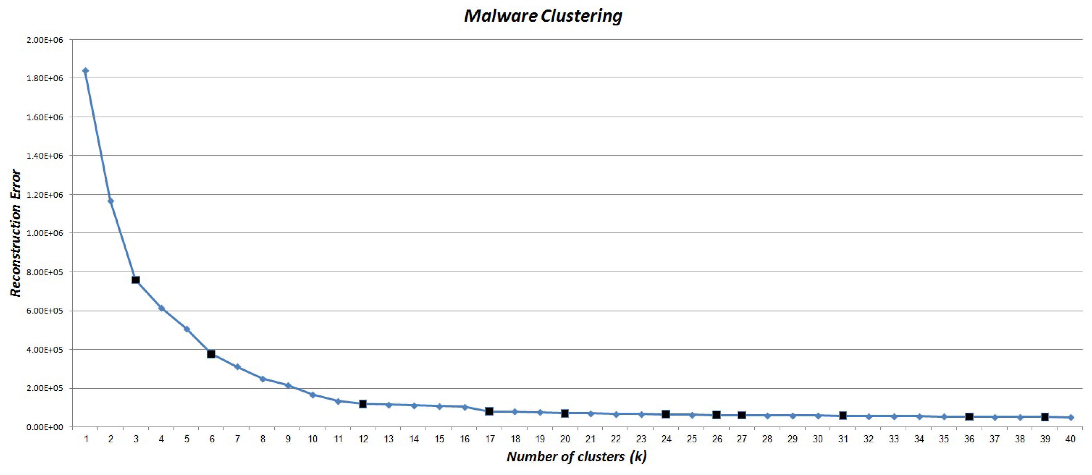
4.1.3. Clustering Action Sequences

Since learning techniques (i.e., HMM) have high performance when input samples are more similar to each other and since malware programs may have different classes of action sequences, we therefore partition all action sequences of malware set to some clusters (i.e., C = { c 1 , c 2 , , c k } ) using complete-link agglomerative hierarchical clustering method [33], where each cluster has high cohesion (i.e., high similarity) and less similarity with other clusters. In the process of clustering, we compute the normalized similarity of every two action sequences A S i and A S j based on Equation (1). Here, E D ( A S i , A S j ) is the edit distance of A S i and A S j , which is computed by the Levenshtein technique [34].
S i m ( A S i , A S j ) = 1 E D ( A S i , A S j ) m a x ( l e n g t h ( A S i ) , l e n g t h ( A S j ) ) .
Algorithm 1 : Preprocessing, generating an action sequence from a system call sequence
Input:
  • S = A system call sequence S = { s 1 , s 2 , , s n } .
Output:
  • A S = An action sequence for system call sequence S.
1:Define an empty array B such that each array element specifies a system call sequence during the execution of algorithm.
2:Initialize A with 26 base actions: A = { v 1 , v 2 , , v 26 }
3:for each s i S do
4: = OS_Handle( s i )            ▷ get the Operating System handle pointer of s i
5:insert( B ( ) , s i )              ▷ for any system call, insert it to B ( )
6:if s i is a releasing system call then ▷ A releasing system call releases the dependent resources and invalidate the handle.
7:  v = Match(A, B ( ) )   ▷ Match B ( ) to the corresponding action in A by a hash function
8:  insert( A S ,v)                  ▷ Insert action (v) to A S
9:end if
10:end for
In the hierarchical clustering method, we plot the reconstruction error as a function of k and look for an elbow. Then, we set k at elbow. k _ S e t denotes the set of all candidate k values that points to the one of the elbow points. In H M 3 a l D , the principle rule is to select the smallest possible k that leads to set of suitable HMMs. We select the smallest k such that: (1) k k _ S e t ; and (2) there is only at most one cluster c i where its members are not similar enough and has just few action sequences. Note that, according to our experience on HMM, if the average similarity of a cluster is less than 0.5, then the corresponding HMM is not converged accurately and leads to a high false alarm rate.

4.1.4. Training HMMs

This section is presented in three parts: (1) input sequences; (2) HMM topology; and (3) yraining.
Input sequences: Action sequences of programs at runtime are observation sequences.
HMM topology: We define the topology of HMMs based on program behavior. Recall that each program consists of three main stages at runtime: (1) initialization; (2) running; and (3) termination. In the initialization stage, each program sets its variables by initial values and allocates its required resources. Thus, we consider this stage as following the serial Bakis topology. In the running stage, programs perform some iterative units of work in the form of conditions and loops. Thus, we consider this stage as following the parallel fully connected (ergodic) topology. The termination stage is somewhat similar to the initialization stage: it publishes the program outputs, deallocates the resources, and terminates the program. Thus, we consider this stage as following the Bakis topology. Figure 2 expresses the novel program behavior-aware HMM topology where the number of states at running stage should be determined.
Training: To learn an HMM, λ c i = ( π c i , A c i , B c i ) , on each malware cluster c i , we must set its initial state probability π c i = { π 1 = 1 } ; its transition probability matrix A c i = { a r j = P ( q t + 1 = S j | q t = S r ) } ; and its observation probability matrix B c i = { b j ( v m ) = P ( O t = v m | q t = S j ) } . To learn HMM λ c i , we first determine the number of states N c i and then initialize A c i and B c i matrices.
According to the proposed program behavior-aware topology (Figure 2), matrix A c i consists of some transitions so the weights of other transitions are zero. Thus, we initialize the values of its non-zero elements randomly with constraint j = 1 N c i a r j = 1 . We initialize matrix B c i randomly with constraint m = 1 M b j ( v m ) = 1 , where M = 26 (i.e., the number of actions). Figure 3 shows a six-state HMM topology and its corresponding matrix A.
To estimate the number of states of each cluster (i.e., N c i ), we compute the number of unique actions that are observed across all sequences corresponding to that cluster. Since they are based on three-stage program behavior-aware topology, the minimum and maximum values of N c i are 3 and 26, respectively.
After calculation of N c i and initialization of A c i and B c i , we apply the Baum–Welch algorithm [29] on each cluster c i to train (the parameters of) its corresponding HMM, λ c i . The Baum–Welch algorithm is an EM-like algorithm and guarantees to converge towards local optima. The Baum–Welch algorithm iterates the E step and the M step, yielding monotonically increasing log-likelihoods, and the algorithm is terminated when the difference of two subsequent log-likelihoods falls below ε that is near to zero or the maximum number of iterations is met. Typically, the algorithm reaches different local maxima or saddle points for different initializations, so we run it multiple times on each cluster c i with different initializations and we finally select HMM, λ c i that has the highest probability. Algorithm 2 shows the steps of training HMMs.

4.1.5. Computing Decision Thresholds

Recall that, in H M 3 a l D , we learn only malware HMMs λ c i , to distinguish between malware and benign programs at detection phase. In this section, we compute a threshold T c i on each HMM λ c i using another fraction of malware action sequences and some benign action sequences. To present well the process of computing the decision thresholds, first we devise some definitions about the HMM threshold concept.
Algorithm 2 : HM3alD-Training phase
Input:
  • C = { c 1 , c 2 , , c k } denotes the set of malware clusters
Output:
  • Trained HMMs set, T r a i n e d H M M s = { λ c 1 , λ c 2 , , λ c k } .
1: T r a i n e d H M M s =                   ▷ an empty set
2:for i = 1 to | C | do
3:  Estimate the number of states ( N c i ) for cluster c i
4:  Initialize π c i , A i and B i using the proposed program behavior-aware topology
5:  Compute λ c i ( A i , B i ) using Baum–Welch algorithm
6:  Add λ c i to T r a i n e d H M M s
7:end for
Definition 1.
For each malware HMM λ c i and its corresponding threshold T c i , the pair ( λ c i , T c i ) is a discriminator such that an observation (action) sequence O l is identified as a malware action sequence if Equation (2) is satisfied. Note that, from now on, we use L P ( O | λ ) instead of l o g ( P ( O | λ ) ) for simplicity.
L P ( O l | λ c i ) T c i = 1 , if O l is a malware action sequence 0 , otherwise , no decision .
In Equation (2), if the output is zero, the result (benign/malware) depends on the other HMM decisions.
Definition 2.
For each malware HMM λ c i , its corresponding rejection rate R c i is a certain fraction of V c i (the validation part of observation sequences of malware cluster c i ) that specifies the maximum permissible error on HMM λ c i . For simplicity, we set R c 1 = R c 2 = = R c k , which leads to different values of the decision thresholds T c i .
Definition 3.
For each malware HMM λ c i , the maximum benign probability P b c i is the greatest log probability that is returned by HMM λ c i for V b , benign action sequences, and is computed by Equation (3).
P b c i = max l { L P ( O l | λ c i ) , for all O l V b } .
The pseudo-code of computing decision thresholds is shown in Algorithm 3.
To compute threshold T c i by using Algorithm 3, we proceed as follows. First, we estimate the log probabilities of the all action sequences belong to V c i and reorder them in ascending order (Lines 3–8). Then, we obtain the malware threshold point t m (Lines 9–10). In many conditions, we find that the P b c i is less than or equal to t m , which means that the corresponding HMM λ c i is sufficiently powerful and returns small log probabilities for benign action sequences. Thus, we finally compute T c i based on this condition (lines 12–16).
Algorithm 3 : Computing decision thresholds for all malware HMMs, λ c i
Input:
  • f r a c r e j = R c 1 = R c 2 = = R c k .
  • V C = { V c 1 , V c 2 , , V c k } and each V c i = { O l } l = 1 | V c i | is the malware validation part of cluster c i .
  • V b = { O l } l = 1 | V b | , is a set of benign action sequences.
  • M a l w a r e _ H M M = { λ c 1 , λ c 2 , , λ c k } , learned HMM set corresponding to malware clusters.
Output:
  • T V = { T c 1 , T c 2 , , T c k } , the threshold vector corresponding to malware HMMs. In other words, { ( λ c 1 , T c 1 ) , ( λ c 2 , T c 2 ) , , ( λ c k , T c k ) }
1:for i = 1 to k do
2: T V =                      ▷ an empty set
3: P V =                      ▷ an empty set
4:for each O l V c i do
5:   P m = L P ( O l | λ c i )
6:  insert( P V , P m )
7:end for
8:sort( P V )                  ▷ sort in ascending order
9: t _ i n d e x =round( f r a c r e j × | P V | )
10: t m = P V ( t _ i n d e x )
11: Compute P b c i by using Equation (3)
12:if P b c i t m then
13:   T c i = P b c i
14:else
15:   T c i = t m
16:end if
17:insert( T V , T c i )
18:end for

4.2. Detection Phase

In the detection phase, as shown in the bottom part of Figure 1, for each program P l at runtime, first its corresponding system call sequence is collected (by detection profiler module), and then its corresponding action sequence O l is generated (by preprocessing module). The induced action sequence O l is given to all learned malware HMMs, { ( λ c 1 , T c 1 ) , ( λ c 2 , T c 2 ) , , ( λ c k , T c k ) } and then H M 3 a l D aggregates their returned results by Algorithm 4. Note that, in Algorithm 4, the forward values are calculated by multiplying small probabilities, and with long action sequences we risk getting underflow. To avoid this, at each time step in the forward algorithm, we normalize the forward values. This technique is presented as Algorithm 5 in Appendix B.
Algorithm 4 applies HMM forward algorithm, forward( O l , λ c i ) on the induced action sequence O l from the running of program P l and it calculates L P ( O l | λ c i ) iteratively. The result will be “Malware” when at least one of the malware HMMs return the probability value f o r w a r d _ v a l u e i greater than or equal to the corresponding threshold value T c i , otherwise it will be “Benign”.

4.3. Time Complexity Analysis

In this subsection, we analyze the time complexity of H M 3 a l D . Recall that H M 3 a l D consists of two main phases: training and detection. In the following, we discuss the time complexity of these steps in detail.

4.3.1. Training Phase

Without loss of generality, we focus on the core of the training phase: Clustering malware action sequences and Training HMMs. For an initial training set X of N t samples generated from the malware program dataset, first we partition X to the k malware cluster. The complexity of the naive complete-link agglomorative algorithm becomes O ( N t 3 ) . Because we exhaustively scan the N t × N t matrix for the largest similarity in each of N t 1 iterations [29]. After clustering malware action sequences, we train HMMs for each of them using Baum–Welch algorithm. if the number of HMM states is N and the length of an action sequence is T, then the time complexity of Baum–Welch algorithm is O ( N 2 T ) [29]. We suppose the average length of each malware action sequence is T and, without loss of generality, the average number of states of all malware clusters is N. Thus, the time complexity of Algorithm 2 becomes O ( N t N 2 T ) . Therefore, we conclude that the overall time complexity of the training phase is O ( N t N 2 T + N t 3 ) .

4.3.2. Detection Phase

In the detection phase, Algorithm 4 applies HMM forward algorithm to the action sequence O l and then aggregates their returns. The time complexity of the forward algorithm is O ( N 2 T ) [29]. Therefore, the time complexity of the detection phase for action sequence O l becomes O ( k N 2 T l ) , where N, T l , and k are the average number of states of all malware clusters, the length of action sequence O l , and the number of malware clusters, respectively.
Algorithm 4 : HM3alD-Detection phase
Input:
  • O l = an induced action sequence O l from the running of program P l in the real environment.
  • M a l w a r e _ H M M = { ( λ c 1 , T c 1 ) , ( λ c 2 , T c 2 ) , , ( λ c k , T c k ) } , learned HMM set corresponding to malware clusters.
Output:
  • program type: Malware/Benign
  •  
  • /*Compute L P ( O l | λ c i ) of action sequence O l with the forward algorithm, for all i = 1 k malware HMMs.*/
1:for i = 1 to k do
2: f o r w a r d _ v a l u e i =forward( O l , λ c i )
/* The forward() is presented as Algorithm 5 in Appendix B.*/
3:if f o r w a r d _ v a l u e i T c i then
4:  return “Malware” & exit              ▷ returns “Malware” and then exit.
5:end if
6:end for
/* If none of the malware HMMs detect the program P l as malware, then the algorithm decides that it is a benign program. */
7:return “Benign”

5. Experimental Evaluation

This section is composed of: (1) introducing dataset; (2) experimental setup; (3) evaluation metrics; (4) presenting the performance of H M 3 a l D with different settings; and (5) the comparison of H M 3 a l D with the state-of-the-art methods.

5.1. Dataset

We used a dataset that consists of 9025 programs, such that 6349 of them are polymorphic malware including bots, worms, viruses and Trojan horses, and the rest (2676) are benign programs. The malware programs are downloaded from VX Heaven virus collection [35] and belong to different families. Each family includes polymorphic samples of a malware that malware writers have made gradually and then they have been registered in VX Heaven’s dataset. For the benign program set, several applications were downloaded from sourceforge.net [36]. These applications also fall into different categories including: video and audio, scientific, educational, games, communications, etc.

5.2. Experimental Setup

Detection in H M 3 a l D was performed at runtime, so recording the system call sequence of a running program must be started when the program begins to run. H M 3 a l D uses Cuckoo sandbox tool which provides an isolated and safe environment to run programs. All the benign and malware programs are executed under Cuckoo sandbox tool [32] on a host, in a virtual environment. A machine with Intel Core i7-4790K processor and 16 GB RAM was used to execute all experiments. We installed the sandbox tool under Ubuntu-13.03 on this machine. The guest OS in this experiment was Windows XP 32 bit. For each program, Cuckoo sandbox restores the guest OS to a safe state, and then, after executing the program, it returns the corresponding system call sequence in JSON format comprehensively. To extract the action set, we developed a set of basic tools in C++ and they are executed in the sandbox environment. We implemented Algorithm 1 as a python script to drive the action sequence of a program from its corresponding system call sequence. We clustered benign (malware) action sequence sets using MATLAB toolbox. We used GHMM library with python wrapper [37] to implement HMM algorithms.
To evaluate the performance of H M 3 a l D , we used cross-validation strategy. The malware program set was randomly partitioned into two parts, 70% for learning malware HMMs λ c i and computing the corresponding malware decision thresholds, and 30% for detection phase. Similarly, the benign program set was randomly partitioned into two parts, i.e. 30% for computing the decision thresholds and 70% for detection phase. To train good HMMs, λ c i , we randomly repeated the cross-validation strategy 10 times. Note that, in the learning process, Algorithm 2 (Baum–Welch algorithm) was repeated 30 times.

5.3. Evaluation Metrics

According to the general definitions, true positive (TP) is the number of truly detected malware programs, true negative (TN) is the number of truly recognized benign programs, false positive (FP) is the number of benign programs that are detected as malware, and false negative (FN) is the number of malware that are detected as benign programs. N m and N b are the number of malware and benign programs, respectively.
Accuracy (Equation (4)) indicates the ratio of malware and benign programs that are truly identified. TP rate (Equation (5)), also called detection rate (DR), is the proportion of malware that are recognized as malware and FP rate (Equation (6)), also called false alarm rate (FAR), is the proportion of benign programs that are incorrectly detected as malware.
A c c u r a c y = T P + T N N m + N b ,
D R = T P N m ,
F A R = F P N b .
Note that one-class classification methods typically suffer from a relatively large value of FAR, because they learn from just samples with the same label [38]. Thus, we intended to maximize DR and Accuracy and minimize FAR.

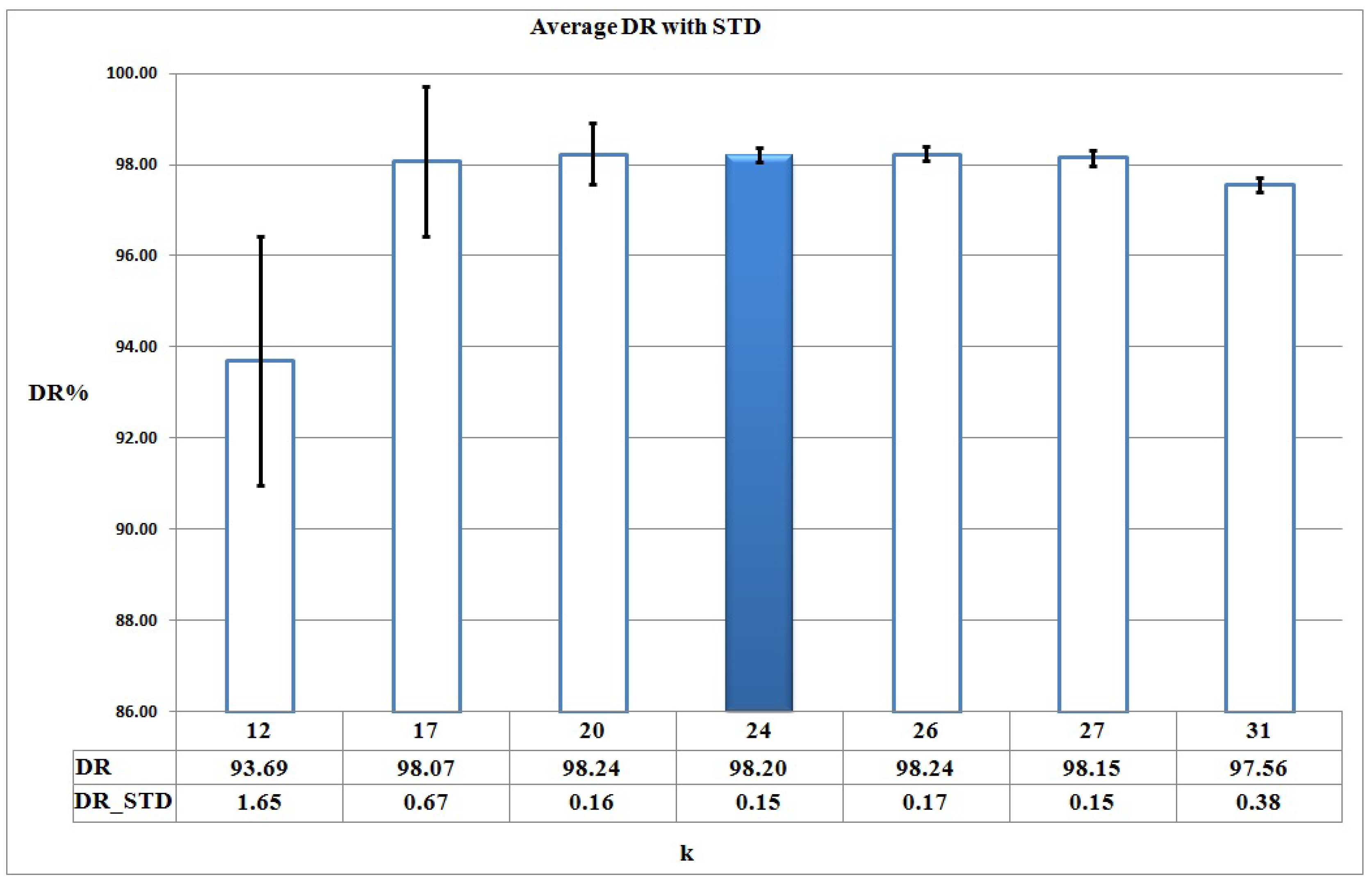
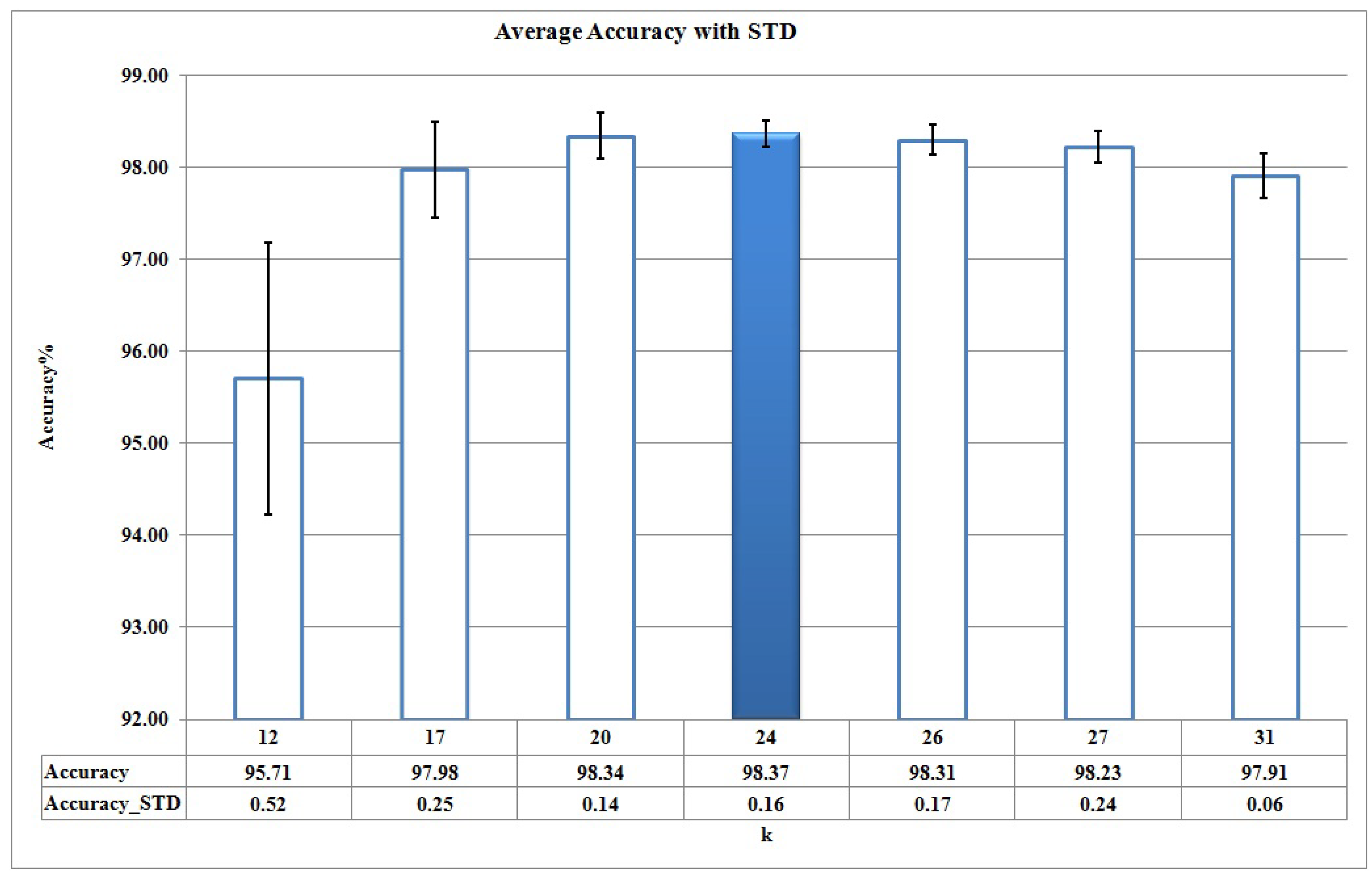
5.4. The Performance of H M 3 a l D

In this section, the different parameters of the proposed method are determined and the results of H M 3 a l D , in different conditions, are presented.

5.4.1. Training Phase

First, we determined the basic parameters such as the number of malware clusters and the number of states for each malware HMM. Then, we clustered malware action sequence sets, and, according to the program based HMM topology (Figure 2), we trained HMMs λ c i on the training part of all malware clusters { X c i } i = 1 k . Finally, we applied Algorithm 3 to compute their corresponding decision thresholds, T c i .
Determining the number of malware clusters
According to the cross-validation strategy, we should choose different values for k in hierarchical agglomerative clustering method. As stated in Section 4.1.3, we applied the complete-link agglomerative clustering method on malware action sequence set. Then, for different values of k, its results in terms of reconstruction error are presented in Figure 4.
As Figure 4 shows, different values can be considered for k. According to the elbow method (see Section 4.1.3), the suitable value of k is one of the candidate values of k _ S e t = {3, 6, 12, 17, 20, 24, 26, 27, 31, 36, 39}. As mentioned in Section 4.1.3, we tended to select the smallest k from the k _ S e t such that it satisfies Conditions (1) and (2). To summarize, Table 1 and Table 2 show the results of two values of k in which k = 17 satisfies the corresponding conditions but k = 12 does not. In other words, by considering k = 12 , we have a cluster (i.e., Cluster 4) such that its size is great and its centroid is less than 0.5 (highlighted row in Table 1). Thus, we can choose one of the k values that is greater than or equal to 17. According to the experiments, which are discussed in Section 5.4.2, the best value of k is 24.
Training HMMs
As in Section 4.1.4, first we calculated the number of states of each cluster (i.e., N c i ). Table 3 presents the number of states for each malware cluster as their corresponding unique actions on training data. According to Figure 2 and Table 3, we design program behavior-aware topology of each HMM, λ c i . Then, by applying Algorithm 3, we computed their corresponding decision thresholds, T c i and finally built all malware HMMs, ( λ c i , T c i ) . Note that we only use 15% of benign action sequences to compute decision thresholds, T c i .

5.4.2. Detection Phase

In the detection phase, we monitor the running of programs and compute the probability of their corresponding action sequences by applying Algorithm 4. In the experiments, we assume the rejection rate f r a c r e j = 0.05 in Algorithm 3 and, by default, we use program behavior-aware topology to train the HMMs, λ c i .
The impact of clustering on the performance of HM3alD
When k, the number of clusters, increases in the clustering process of H M 3 a l D , the corresponding reconstruction error decreases and also the number of clusters is increased, so it means we should learn more HMMs. It means we should trade off between k and the set of {DR, FAR, Accuracy} metrics derived from corresponding HMMs, ( λ c i , T c i ) . Figure 5, Figure 6 and Figure 7 show the average and STD (Standard deviation) of DR, FAR, and Accuracy of H M 3 a l D for different candidate values of k, based on Figure 4 respectively.
As it can be seen in Figure 5, Figure 6 and Figure 7, DR, FAR, and Accuracy metrics for k = 24 are better in comparison with the results for other k values. This happens because, when considering a small number of clusters (for example k = 3, 6, 12), malware action sequences that are less similar are assigned to the same cluster, so no suitable HMMs are learned. Thus, the learned HMMs are neither able to detect malware programs properly nor discriminate between malware and benign programs as good as possible. On the other hand, the large number of clusters increases the complexity of H M 3 a l D and causes each cluster to have too few action sequences (for example, k = 26, 27, 31).
Cross-validation results show that 19 of 24 malware HMMs (i.e., 80% of the learned HMMs) compute their decision thresholds based on the maximum benign probability P b c i in Algorithm 3. This fact means that HMMs are trained suitably and effectively discriminate between malware and benign action sequences.
The impact of program behavior-aware topology
Figure 8 shows the comparison results of H M 3 a l D and H M 3 a l D ̲ R (without program behavior-aware topology). As it is seen, H M 3 a l D ̲ R dramatically increases FAR. In other words, H M 3 a l D that preserves program behavior-aware topology, effectively reduces FAR 227%, which is hard work without any impact on DR.
The impact of expressing system call sequences as action sequences
To explain the importance of the action sequences, we examine the proposed method by considering the raw system call sequences (called H M 3 a l D ̲ S ) instead of the action sequences. H M 3 a l D ̲ S ̲ R denotes the random topology version of H M 3 a l D ̲ S . Recall that it is shown that methods based on raw system call sequences produce many false positives [39], and not considering their parameters such as frequency and arguments would result in high false alarm rate [40,41]. Figure 9 shows the efficiency of H M 3 a l D in comparison with H M 3 a l D ̲ S and H M 3 a l D ̲ S ̲ R in terms of FAR and DR. It is seen that in H M 3 a l D , FAR is decreased 453%, and DR is increased 5.8%. As an important result, using action sequences in H M 3 a l D achieves high DR and low FAR, that is a difficult task in HMM methods as a one-class classifier approach.

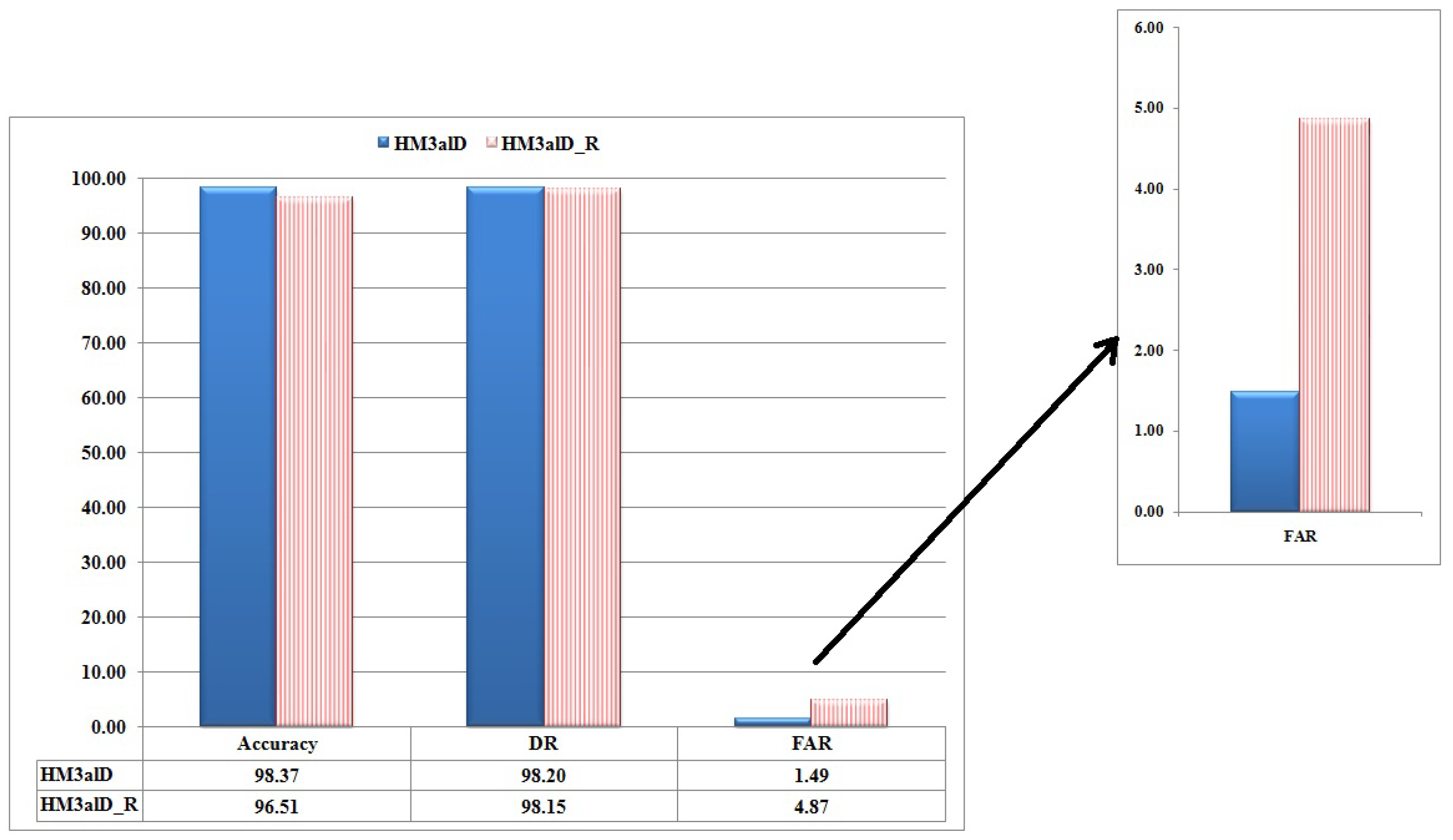
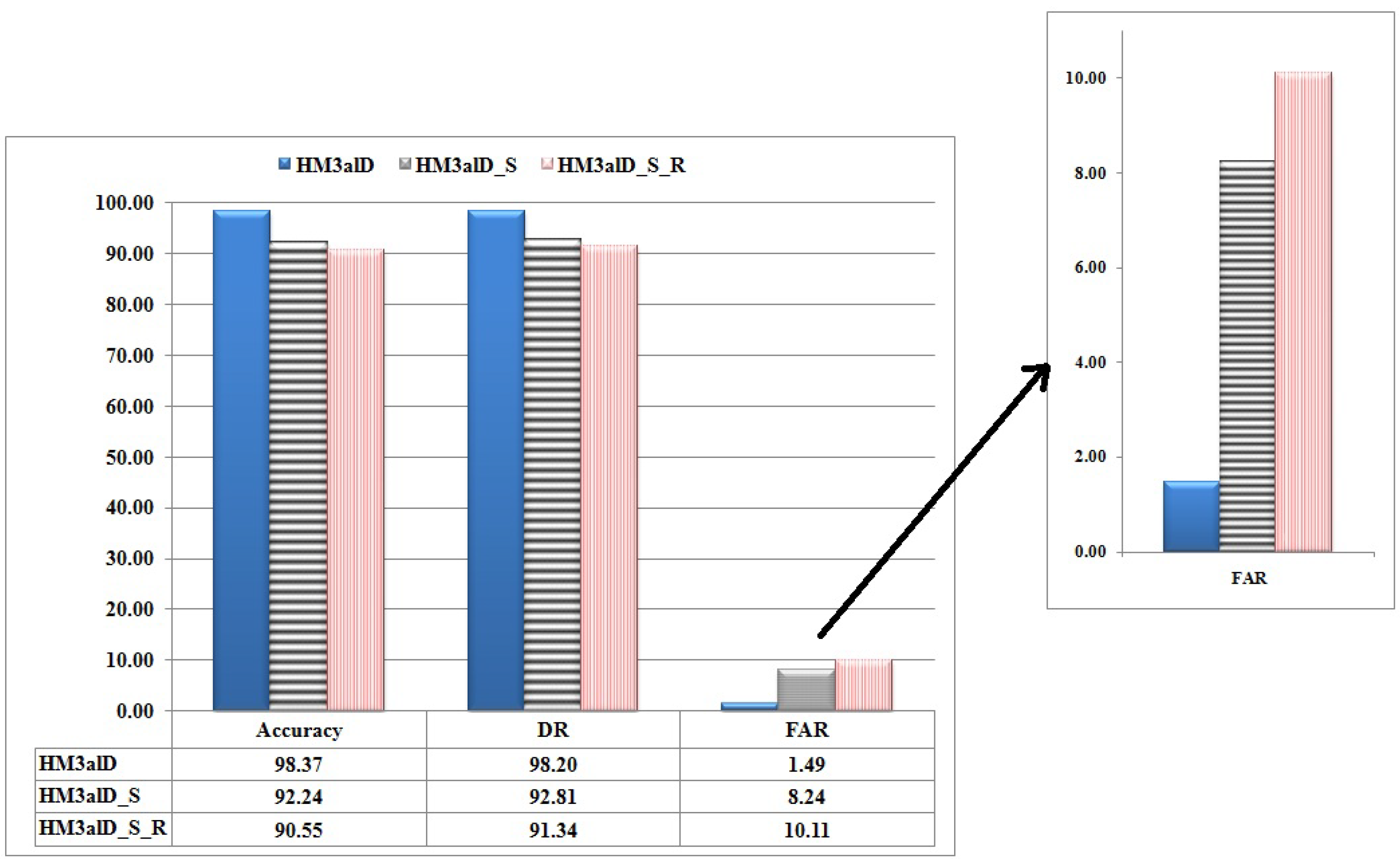
5.5. Comparing with Other Work

In this section, the performance of H M 3 a l D in terms of DR, FAR, and Accuracy is compared to important previous works. For fair comparison, we consider the number of dataset members same as the compared methods when we train HMMs of H M 3 a l D . To express the detection performance of H M 3 a l D , we compare H M 3 a l D to dynamic malware detection methods and show the corresponding results in Table 4. Moreover, Table 5 shows the results of H M 3 a l D in comparison with static malware detection methods. As shown in Table 4 and Table 5, H M 3 a l D outperforms all dynamic and static malware detection methods especially in term of FAR that is a hard work to decrease it without affecting DR.
Expressing the behavior of a malware program leads to detect its polymorphic instances, effectively. H M 3 a l D tries to extract realistic behavior of malware from polymorphic instances. First, H M 3 a l D abstracts malware behavior by using high-level action sequences instead of system call sequences. Then, it clusters similar malware action sequences leading to integrate polymorphic instances of a malware. Finally, H M 3 a l D models the realistic behavior of each malware cluster using HMM. Thus, H M 3 a l D provides a high detection rate and low false rate in comparison with other work.
Note that a false positive occurs when H M 3 a l D erroneously labels a benign program as malware. If a malware detector blocks access or deletes a program or file that is vital to the proper functioning of some system programs, those may become unusable and, in some cases, the deletion may render a system unstable, although the anti-malware methods try to reduce FAR to zero. For Virus Bulletin [42], “the `no false positives’ rule is one of the main requirements for certification in the VB100 test process”. AV-Comparatives [43] considers false positives “an important measurement for AV quality”, and an important factor in determining the reliability of a product, besides its detection capabilities. Thus, we introduce new metric, P e n a l i z e d D R , as Equation (7).
P e n a l i z e d D R = D R α F A R ,
We analyze the impact of α by increasing it from 0 to 10 in increments of 0.5. Figure 10 and Figure 11 show the results of P e n a l i z e d D R for H M 3 a l D and current dynamic and static methods, respectively.
The important findings from the results shown in Figure 10 and Figure 11 are as follows: (1) FAR is the most important and impressive measurement for malware detection methods; (2) high DR is not enough to have a good result and its effectiveness depends on FAR; and (3) high FAR significantly reduces the usefulness and applicability of such methods. According to Table 4 and Table 5, and Figure 10 and Figure 11, the performance of H M 3 a l D is always higher than the other methods in terms of DR and Accuracy and is significantly better than the other methods in term of FAR.

6. Analysis and Discussion

We analyze the proposed method, H M 3 a l D , from three aspects: action sequences, HMM topology, and the impact of clustering and decision thresholds on learned HMMs.
Expressing the realistic behavior of a malware program is definitely effective in detecting its polymorphic instances. Therefore, it is crucial to have an effective yet feasible way to express malware behavior. According to experimental results, raw data from malware at runtime that is merely a sequence of system calls is too fine-grained to be helpful in expressing the realistic behavior of a suspicious program. Therefore, H M 3 a l D defines and operates on some high-level “actions” (i.e., read file, write file, send data, and remove a registry key) where a sequence of these actions represents a more meaningful behavior. Results shown in Figure 9 indicate that, without a high level action sequence, we would not find acceptable performance for the proposed method especially in term of FAR.
In HMM, designing HMM topology is really important. Taking this fact into account, H M 3 a l D employs a special HMM topology to learn malware behaviors in coarse grain. The resulting HMM topology is built based on a triple-stage (initialization, running, and termination) execution of a program. This approach has a great impact on training and building suitable HMMs and, compared to the other similar methods (e.g., [13]), H M 3 a l D provides a drastic decrease in FAR without any alteration in DR. As Figure 8 shows, if we use a random topology rather than a program behavior-aware topology in the training phase, the learned HMMs are not much effective.
Furthermore, a key feature of H M 3 a l D is that we train each HMM using only malware action sequences (i.e., without using any benign action sequences) that leads to reducing the complexity of H M 3 a l D dramatically, in the training phase. Note that, in computing the HMM decision thresholds, we use malware and a few benign action sequences.
Clustering action sequences makes it possible to put similar action sequences in the same group. Results indicate that without proper clustering of action sequences, we cannot train suitable HMMs in the training phase, which leads to unacceptable malware detection results.
Our implementation of H M 3 a l D shows great promise in DR and especially in FAR even when the number of programs goes beyond the capability of some current methods.

7. Conclusions and Future Work

In this study, we showed that it is possible to employ HMMs to detect polymorphic malware in a dynamic manner. In this paper, we propose a novel dynamic detection method, named H M 3 a l D , based on HMM to detect polymorphic malware. We show that the proposed method could effectively distinguish between benign and malware programs. H M 3 a l D was trained only by malware action sequences to detect polymorphic malware on the host side at runtime.
In the future, we will work on the applications of this method in classifications of malware programs, detecting anomalies and generating behavioral signatures. We will also try to perform the detection at the early stages of program execution, as much as possible.

Author Contributions

A.T. is the author who mainly contributed to this research, performing experiments, and writing the manuscript. S.J. read and approved the final manuscript, and reviewed the results.

Funding

This research received no external funding.

Conflicts of Interest

The authors declare no conflict of interest.

Appendix A. Mapping a Subsequence of System Calls to Actions

High-level actions derived from subsequences of system calls are classified into seven sets:
  • File Actions include “write file”, “read file”, “delete file”, “execute file”, “copy file”, and “move file”.
  • Registry Actions indicate the program behavior regarding the registry of Windows operating system (OS), which includes writing, reading, and deleting in the registry.
  • Service Actions relate to the registered services in Windows OS. These actions include creating, deleting, and executing a service in Windows.
  • Network Actions cover the behavior of executing sample in the transport layer. This Action set is formed based on the state diagram in the TCP protocol, which includes opening and closing a connection (socket), listening on a socket, binding a socket, accepting a socket, sending and receiving on a socket, etc.
  • Internet Actions include all actions that occur during communications of a running program in the Application Layer. These actions include opening a session, session connection, and sending and reading files via the network.
  • System Actions consist of the sequence of system calls which express a system operation to begin the execution. Load library, memory allocation, address allocation to procedures, etc. are some examples of system actions.
  • Process Actions include all the actions related to process and threads, (e.g., creating, executing, and killing a thread.)
For example, we map the subsequence of system call {NTCreateFile, NTOpenFile, NTReadFile, NTReadFile, NTReadFile, NTCloseFile} to the action R e a d F i l e .

Appendix B. The Forward Algorithm

Algorithm 5 : Forward algorithm
It implements the scaled forward algorithm and returns:
(1) log( P ( O | λ ) ); (2) scale factor set F = { f 1 , f 2 , , f T } ; and (3) scale forward variables, α ^ t ( i ) .
Input:
  • O = an induced action sequence { O 1 , O 2 , , O T } corresponding to a program P
  • A = state transition probability matrix with the number of states (N)
  • B = observation probability matrix
Outputs:
  • scaled forward value = l o g P ( O | λ )
  • scale factor set F = { f 1 , f 2 , , f T }
  • scale forward variables, α ^ t ( i ) for all i = 1 N and t = 1 N
Initialization:
1: f 1 = 0
2:for i = 1 to N do
3: α 1 ( i ) = π i b i ( O 1 )
4: α 1 ( i ) = α 1 ( i )
5: f 1 = f 1 + α 1 ( i )
6:end for
7: f 1 = 1 f 1
8:for i = 1 to N do
9: α ^ 1 ( i ) = f 1 α 1 ( i )
10:end for
Induction:
11:for t = 2 to T do
12: f t = 0
13:for i = 1 to N do
14:   x = 0
15:  for j = 1 to N do
16:    x = x + α ^ t 1 ( j ) a j i
17:  end for
18:   α t ( i ) = b i ( O t ) x
19:   f t = f t + α t ( i )
20:end for
21: f t = 1 f t
22:for i = 1 to N do
23:   α ^ t ( i ) = f t α t ( i )
24:end for
25:end for
Termination
26: l o g _ p = 0
27:for t = 1 to T do
28: l o g _ p = l o g _ p + l o g ( f t )
29:end for
30: l o g _ p = l o g _ p
31:return l o g _ p

References

  1. Kang, B.; Han, K.S.; Kang, B.; Im, E.G. Malware categorization using dynamic mnemonic frequency analysis with redundancy filtering. J. Digit. Investig. 2014, 11, 323–335. [Google Scholar] [CrossRef]
  2. Shin, S.; Zhaoyan, X.; Guofei, G. EFFORT: A new host–network cooperated framework for efficient and effective bot malware detection. Comput. Netw. 2013, 57, 2628–2642. [Google Scholar] [CrossRef] [Green Version]
  3. Symantec. Available online: http://www.symantec.com/threatreport/ (accessed on 25 June 2018).
  4. Lu, H.; Wang, X.; Zhao, B.; Wang, F.; Su, J. ENDMal: An anti-obfuscation and collaborative malware detection system using syscall sequences. J. Math. Comput. Model. 2013, 58, 1140–1154. [Google Scholar] [CrossRef]
  5. Shahid, A.; Horspool, R.N.; Traore, I.; Sogukpinar, I. A framework for metamorphic malware analysis and real-time detection. J. Comput. Secur. 2015, 48, 212–233. [Google Scholar]
  6. Cha, S.K.; Moraru, I.; Jang, J.; Truelove, J.; Brumley, D.; Andersen, D.G. SplitScreen: Enabling efficient, distributed malware detection. J. Commun. Netw. 2011, 13, 187–200. [Google Scholar] [CrossRef] [Green Version]
  7. Egele, M.; Scholte, T.; Kirda, E.; Kruegel, C. A survey on automated dynamic malware-analysis techniques and tools. ACM Comput. Surv. 2012, 44, 6. [Google Scholar] [CrossRef]
  8. Bruschi, D.; Martignoni, L.; Monga, M. Code normalization for self-mutating malware. IEEE J. Secur. Priv. 2007, 5, 46–54. [Google Scholar] [CrossRef]
  9. Chandola, V.; Banerjee, A.; Kumar, V. Anomaly detection: A survey. J. ACM Comput. Surv. 2009, 41, 15. [Google Scholar] [CrossRef]
  10. Grill, M.; Pevny, T. Learning combination of anomaly detectors for security domain. Comput. Netw. 2016, 107, 55–63. [Google Scholar] [CrossRef]
  11. Preda, M.D.; Christodorescu, M.; Jha, S.; Debray, S. A semantics-based approach to malware detection. ACM Trans. Program. Lang. Syst. 2008, 30, 25. [Google Scholar] [CrossRef]
  12. Faruki, P.; Laxmi, V.; Gaur, M.S.; Vinod, P. Mining control flow graph as API call-grams to detect portable executable malware. In Proceedings of the ACM International Conference on Security of Information and Networks, Jaipur, India, 25–27 October 2012. [Google Scholar]
  13. Kalbhor, A.; Austin, T.H.; Filiol, E.; Josse, S.; Stamp, M. Dueling hidden Markov models for virus analysis. J. Comput. Virol. Hacking Tech. 2015, 11, 103–118. [Google Scholar] [CrossRef]
  14. Wong, W.; Stamp, M. Hunting for metamorphic engines. J. Comput. Virol. 2006, 2, 211–229. [Google Scholar] [CrossRef]
  15. Austin, T.H.; Filiol, E.; Josse, S.; Stamp, M. Exploring hidden markov models for virus analysis: A semantic approach. In Proceedings of the 46th Hawaii International Conference on System Sciences, Wailea, HI, USA, 7–10 January 2013. [Google Scholar]
  16. Song, F.; Touili, T. Efficient malware detection using model-checking. J. Formal Methods (FM) 2012, 7436, 418–433. [Google Scholar]
  17. Ding, Y.; Yuan, X.; Tang, K.; Xiao, X.; Zhang, Y. A fast malware detection algorithm based on objective-oriented association mining. J. Comput. Secur. 2013, 39, 315–324. [Google Scholar] [CrossRef]
  18. Hellal, A.; Lotfi, B.R. Minimal contrast frequent pattern mining for malware detection. J. Comput. Secur. 2016, 62, 19–32. [Google Scholar] [CrossRef]
  19. Park, Y.; Reeves, D.S.; Stamp, M. Deriving common malware behavior through graph clustering. J. Comput. Secur. 2013, 39, 419–430. [Google Scholar] [CrossRef]
  20. Shahzad, F.; Shahzad, M.; Farooq, M. In-execution dynamic malware analysis and detection by mining information in process control blocks of Linux OS. J. Inf. Sci. 2013, 231, 45–63. [Google Scholar] [CrossRef]
  21. Elhadi, A.A.E.; Maarof, M.A.; Barry, B.I.; Hamza, H. Enhancing the detection of metamorphic malware using call graphs. J. Comput. Secur. 2014, 46, 62–78. [Google Scholar] [CrossRef]
  22. Shehata, G.H.; Mahdy, Y.B.; Atiea, M.A. Behavior-based features model for malware detection. J. Comput. Virol. Hacking Tech. 2015, 12, 59–67. [Google Scholar]
  23. Salehi, Z.; Sami, A.; Ghiasi, M. MAAR: Robust features to detect malicious activity based on API calls, their arguments and return values. J. Eng. Appl. Artif. Intell. 2017, 59, 93–102. [Google Scholar] [CrossRef]
  24. Christodorescu, M.; Jha, S.; Kruegel, C. Mining specifications of malicious behavior. In Proceedings of the the 6th Joint Meeting of the European Software Engineering Conference and the ACM SIGSOFT Symposium on the Foundations of Software Engineering, Dubrovnik, Croatia, 3–7 September 2007. [Google Scholar]
  25. Kolbitsch, C.; Comparett, P.M.; Kruegel, C.; Kirda, E.; Zhou, X.; Wang, X. Effective and efficient malware detection at the end host. In Proceedings of the International Conference on USENIX Security Symposium, Montreal, QC, Canada, 10–14 August 2009. [Google Scholar]
  26. Ding, Y.; Xiaoling, X.; Sheng, C.; Ye, L. A malware detection method based on family behavior graph. J. Comput. Secur. 2018, 73, 73–86. [Google Scholar] [CrossRef]
  27. Schrittwieser, S.; Stefan, K.; Johannes, K.; Georg, M.; Edgar, W. Protecting software through obfuscation: Can it keep pace with progress in code analysis? ACM Comput. Surv. 2016, 49, 4:1–4:37. [Google Scholar] [CrossRef] [Green Version]
  28. Cohen, Y.; Danny, H. Scalable Detection of Server-Side Polymorphic Malware. Knowl.-Based Syst. 2018, 156, 113–128. [Google Scholar] [CrossRef]
  29. Alpaydin, E. Introduction to Machine Learning; MIT Press: London, UK, 2014. [Google Scholar]
  30. Camastra, F.; Vinciarelli, A. Machine Learning for Audio, Image, and Video Analysis; Springer: London, UK, 2008. [Google Scholar]
  31. Francis, H.; Chen, H.; Ristenpart, T.; Li, J.; Su, Z. Back to the future: A framework for automatic malware removal and system repair. In Proceedings of the 22nd Annual Computer Security Applications Conference, Miami Beach, FL, USA, 11–15 December 2006. [Google Scholar]
  32. Cuckoo Foundation. Available online: https://www.cuckoosandbox.org (accessed on 25 June 2018).
  33. Murtagh, F. A survey of recent advances in hierarchical clustering algorithms. Comput. J. 1983, 26, 354–359. [Google Scholar] [CrossRef]
  34. Yujian, L.; Bo, L. A normalized Levenshtein distance metric. IEEE Trans. Pattern Anal. Mach. Intell. 2007, 29, 1091–1095. [Google Scholar] [CrossRef] [PubMed]
  35. VxHeavens. Available online: http://vxheaven.org/vl.php (accessed on 1 March 2016).
  36. Sourceforge. Available online: https://sourceforge.net/ (accessed on 25 June 2018).
  37. GHMM Library. Available online: http://www.ghmm.org/ (accessed on 25 June 2018).
  38. Giacinto, G.; Perdisci, R.; Del Rio, M.; Roli, F. Intrusion detection in computer networks by a modular ensemble of one-class classifiers. J. Inf. Fusion 2008, 9, 69–82. [Google Scholar] [CrossRef] [Green Version]
  39. Lanzi, A.; Balzarotti, D.; Kruegel, C.; Christodorescu, M.; Kirda, E. Accessminer: Using system-centric models for malware protection. In Proceedings of the 17th ACM conference on Computer and communications security, Chicago, IL, USA, 4–8 October 2010; pp. 399–412. [Google Scholar]
  40. Das, S.; Liu, Y.; Zhang, W.; Chandramohan, M. Semantics-Based Online Malware Detection: Towards Efficient Real-Time Protection Against Malware. IEEE Trans. Inf. Forensics Secur. 2016, 11, 289–302. [Google Scholar] [CrossRef]
  41. Maggi, F.; Matteucci, M.; Zanero, S. Detecting intrusions through system call sequence and argument analysis. IEEE Trans. Dependable Secur. Comput. 2010, 7, 381–395. [Google Scholar] [CrossRef]
  42. Virus Bulletin. Available online: https://www.virusbulletin.com (accessed on 25 June 2018).
  43. AV-Comparatives. Available online: http://www.av-comparatives.org/false-alarm-tests (accessed on 1 September 2016).
Figure 1. The architecture of H M 3 a l D .
Applsci 08 01044 g001
Figure 2. The proposed program behavior-aware HMM topology in H M 3 a l D .
Applsci 08 01044 g002
Figure 3. A six-state program behavior-aware HMM topology and its corresponding transition probability matrix A.
Applsci 08 01044 g003
Figure 4. Variation of reconstruction error for different number of malware clusters. Black points shows candidate k values.
Applsci 08 01044 g004
Figure 5. DR for different candidate values of k based on Figure 4.
Applsci 08 01044 g005
Figure 6. FAR for different candidate values of k based on Figure 4.
Applsci 08 01044 g006
Figure 7. Accuracy for different candidate values of k based on Figure 4.
Applsci 08 01044 g007
Figure 8. The performance comparison of H M 3 a l D with and without the program behavior-aware topology for k = 24 and f r a c r e j = 0.05 .
Applsci 08 01044 g008
Figure 9. The performance comparison of H M 3 a l D (for k = 24 ), H M 3 a l D ̲ S (for k = 26 ) and H M 3 a l D ̲ S ̲ R (for k = 26 ).
Applsci 08 01044 g009
Figure 10. P e n a l i z e d D R for H M 3 a l D and current dynamic methods: (a) Salehi (2017) [23]; and (b) Shehata (2015) [22].
Applsci 08 01044 g010
Figure 11. P e n a l i z e d D R for H M 3 a l D and current static methods: (a) Shahid (2015) [5]; (b) Furuki (2012) [12]; (c) Ding (2013) [17]; and (d) Kalbhor (2015) [13]. Note that we estimated FAR value of Ding work [17] from DR and Accuracy.
Applsci 08 01044 g011
Table 1. The malware clusters for k = 12 .
Cluster No.Cluster SizeCentroid
12730.65
216380.59
32430.89
43180.41
53110.82
62680.81
73760.56
85100.62
93720.73
105880.68
115920.83
128600.95
Table 2. The malware clusters for k = 17 .
Cluster No.Cluster SizeCentroid
14680.79
211700.61
3540.13
42640.58
54920.90
61000.63
7920.72
82840.59
93080.79
10640.56
112730.65
122430.89
133110.82
142680.81
155100.62
165880.68
178600.95
Table 3. The number of HMM states for k = 24 .
Cluster No.123456789101112131415161718192021222324
N c i 21221718161517232623152120192218142323101216219
Table 4. Comparison of H M 3 a l D with current dynamic malware detection methods.
ApproachesDataset Size (Benign/Malware)DR(%)FAR(%)Accuracy (%)
Shahzad (2013) [20]105/11493.7096.65
H M 3 a l D 105/1141000100
Elhadi (2014) [21]98/41697.57098.05
H M 3 a l D 98/4161000100
Salehi (2017) [23]1359/300998.44.6
H M 3 a l D 1359/300998.891.1298.88
Shehata (2015) [22]2000/200097.62.3796.89
H M 3 a l D 2000/200098.831.1898.87
Table 5. Comparison of H M 3 a l D with the current static malware detection methods.
MethodsDataset Size (Benign/Malware)DR(%)FAR(%)Accuracy (%)
Kalbhor (2015) [13]370/76088.950.297.58
H M 3 a l D 370/76099.120.2399.38
Song (2012) [16]8/20010012.599.52
H M 3 a l D 8/2001000100
Shahid (2015) [5]2330/102098.94.5
H M 3 a l D 2330/102098.991.2798.85
Furuki (2012) [12]2595/363998.42.797.85
H M 3 a l D 2595/363998.811.3698.70
Ding (2013) [17]3760/441097.391.2
H M 3 a l D 2676/441098.791.8598.39

