Stabilization of Underactuated Surface Vessels: A Continuous Fractional Power Control Method

Abstract

This paper investigates the problem of global asymptotic stabilization of underactuated surface vessels (USVs) whose dynamics features off-diagonal inertia and damping matrices. By using input and state transformations, the dynamic model of USV is converted into an equivalent system consisting of two cascade connected subsystems. For the transformed system, a continuous fractional power control framework is given to achieve global asymptotic stabilization of USVs. Then, the convergence under this framework is analyzed showing that the rate can be improved by adjusting the fractional power term. Finally, a continuous control algorithm is proposed to guarantee the global convergence rate of the USV system. Simulations are given to demonstrate the effectiveness of the presented method.

1. Introduction

1.1. Background Material

Dynamic positioning of underactuated surface vessels (USV) plays an important role in many offshore applications such as cable laying, mine sweeping, platform supplying, rock dumping and, especially, oil field operations like drilling, pipe-laying and diving support. Critical to the dynamic positioning problem of an USV is its capability for accurate and reliable control subject to environmental disturbances as well as to configuration related changes. It is an underactuated control problem, since the number of independent actuators of the system is less than that of the degree of freedom. In this paper, we consider the stabilization problem of an USV that has no side thruster but only two independent main thrusters to provide surge force and yaw moment. The challenging problem is how to design a feedback control law that stabilizes both the position and the orientation of the vessel using only two available control inputs.

1.2. Formulation of the Problem of Interest for This Investigation

It is shown in [1] that USVs cannot be asymptotically stabilized to a desired equilibrium point using time-invariant continuous feedback law, since the dynamic models of USVs result in systems with nonholonomic constraints that does not satisfy Brockett’s necessary condition in [2]. Moreover, the control methods developed for stabilizing nonholonomic systems cannot be directly used to stabilize USVs, since the dynamics of an USV are not drift-less [3]. For these reasons, the stabilization problem of USVs has been an active research topic for decades and various approaches can be found in the literature.

1.3. Literature Survey

To name some, in the reference [4], a discontinuous feedback stabilization control law with $\sigma$ process was proposed. In the reference [1], Pettersen presented a discontinuous control law via homogeneous-transformation, which can stabilize the system into a neighborhood of the equilibrium point. Then in the reference [5] an improved scheme was given to increase the convergence rate of the method in the reference [1]. Although these results can stabilize underactuated surface vessels, they are limited by the singular point problem. To deal with this problem, in references [6,7], switching control methods that can avoid singularity by controlling the convergence rate were proposed. In the reference [8], Zhang also gave a switching control law that has no singular point problem.

The above research works have one thing in common, namely, the control laws are discontinuous and difficult for implementation in engineering systems. Therefore, considerable research attention has been paid to USV stabilization with a continuous control law. For example, in the reference [9], Pettersen proposed a continuous control law based on backstepping method that can guarantee semi-global asymptotic stability. In references [10,11], backstepping methods are investigated to ensure global asymptotic stability of USVs. In the reference [12], a simpler backstepping control law is proposed with the aid of a state transformation first presented in the reference [13]. In references [14,15,16], backstepping methods are given to asymptotically stabilize the USV system with off-diagonal dynamics and unknown model parameters respectively. Although the methods in references [10,11,12,14,15,16] asymptotically stabilize USVs with continuous control laws, backstepping-based control laws are difficult to guarantee convergence rates (especially near the origin). In fact, the second and third methods in the reference [12] can achieve global exponential convergence to the origin; however, they can not guarantee even local asymptotic stability of the origin. Therefore, it is necessary to asymptotically stabilize the system by a continuous method with a faster rate.

As is well known, fractional power control can improve convergence performance and robustness near the origin [17,18,19]. However, most methods of fractional power control cannot be directly used to stabilize USVs, since the dynamics of USVs are strongly nonlinear and coupled. Although in [8], a finite-time switching scheme for stabilizing USVs based on fractional power control was provided, the method is discontinuous. To the best of the authors’ knowledge, the stabilization of USVs by continuous fractional power control law has not been solved.

1.4. Scope and Contribution of This Study

Motivated by the above observations, this paper aims to address the stabilization problem of USVs with off-diagonal dynamics using a continuous fractional power control method. A transformation is introduced from references [8,20] to transform the system model to a simple pure cascade form, which is realized by a sequence of coordinate transformations including input transformation and diffeomorphism state transformation. The main contributions of this paper are twofold:

(1)

For the transformed system, a novel continuous fractional power control framework is derived by combining the fractional power control scheme with the Lyapunov method and Barbalat Lemma, which can globally asymptotically stabilize the USVs. What makes the framework interesting is that, compared with the backstepping method, there is no need for the above controller to track any smooth state trajectories, so that the fractional power term can be used to improve the convergence rate (especially near the origin).

(2)

Then for the aforementioned controller, the effects of parameters on the convergence rate are analyzed, which shows that we can improve the rate both near and far from the origin by adjusting the fractional power term. On this basis, we construct a continuous control algorithm of the USVs and prove that the control algorithm can improve the overall convergence rate. The presented fractional power control method is simpler and faster near the origin than methods in references [10,11,12].

1.5. Organization of the Paper

This paper is organized as follows. Section 2 is the modeling of underactuated surface vessels and the objective. Section 3 contains the input and state transformations by which the underactuated USV model is transformed into two cascade subsystems. Section 4 gives the continuous fractional power control framework and the analysis of convergence. Also in this section, proofs of global asymptotic stability are also given. Numerical simulations and discussions are given in Section 5.

2. System Modeling and the Objective

2.1. Modeling

The complete configuration of an USV (the position and orientation) can be described by six independent coordinates, or six degree of freedom (DOF), i.e., surge, sway, heave, roll, pitch and yaw. It is common to reduce the six-DOF model to a three-DOF one with surge, sway and yaw, since the other three states (heave, roll and pitch) are open loop stable for most ships and hence are neglected. Define the state vector as $\eta ={[x,y,\psi ]}^T$, where $[x,y]\in R^2$ is the position of the vessel in the inertial frame, and $\psi \in [0,2\pi ]$ is the heading angle of the ship relative to the geographic north. Then model of the USV can be the same as that of [21,22,23]:

$$\begin{array}{c}\hfill \left\{\begin{array}{cc}\hfill \dot{x}=& u\cos \psi -v\sin \psi ,\hfill \\ \hfill \dot{y}=& u\sin \psi +v\cos \psi ,\hfill \\ \hfill \dot{\psi }=& r,\hfill \end{array}\right.\end{array}$$

(1a)

and

$$\begin{array}{c}\hfill \left\{\begin{array}{cc}\dot{u}\hfill & =-{\displaystyle \frac{d_{11}}{m_{11}}}u+{\displaystyle \frac{m_{22}}{m_{11}}}vr+{\displaystyle \frac{m_{23}+m_{32}}{2m_{11}}}{r}^2+{\displaystyle \frac{{\tau }_u}{m_{11}}},\hfill \\ \hfill \dot{v}& =-{\displaystyle \frac{d_{22}}{m_{22}}}v-{\displaystyle \frac{m_{11}}{m_{22}}}ur-{\displaystyle \frac{d_{23}}{m_{22}}}r-{\displaystyle \frac{m_{23}}{m_{22}}}\dot{r},\hfill \\ \dot{r}\hfill & =\frac{m_{22}}{m_{22}{m}_{33}-m_{32}{m}_{23}}\{{\tau }_r+\frac{uv}{m_{22}}(m_{11}{m}_{22}-m_{22}^2)\hfill \\ & +\frac{ur}{m_{22}}\left[m_{11}{m}_{32}-\frac{m_{22}(m_{23}-m_{32})}{2}\right]\hfill \\ & +(m_{32}{d}_{22}-m_{22}{d}_{32})\frac{v}{m_{22}}\hfill \\ & -(m_{22}{d}_{33}-m_{32}{d}_{23})\frac{r}{m_{22}}\},\hfill \end{array}\right.\end{array}$$

(1b)

where $u,v,r$ are, respectively, the forward velocity, the transverse velocity and the angular velocity in yaw, $m_{11},m_{22},m_{23},m_{32}$ and $m_{33}$ are the inherent and added mass of the vehicle, $d_{11},d_{22},d_{23},d_{32}$ and $d_{33}$ are the hydrodynamic damping coefficients, ${\tau }_u$ and ${\tau }_r$ are the force in surge and the torque in yaw. The USV considered has bilateral asymmetry, so $m_{23}=m_{32}\ne 0$ and $d_{23}\ne d_{32}\ne 0$. The details are in Figure 1.

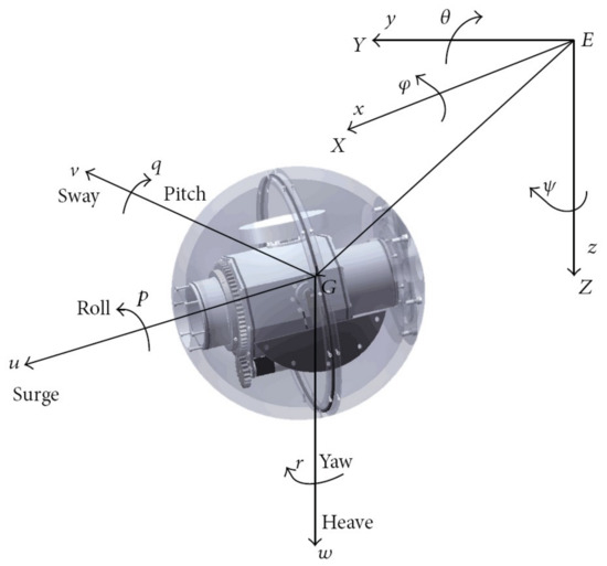
Figure 1. Earth-fixed and body-fixed coordinate systems.

2.2. The Objective

The objective of this paper is to establish a control methodology that can globally asymptotically stabilize the USV system in (1), namely, the following holds true for any initial conditions

$$\begin{array}{c}\hfill \begin{array}{c}\hfill \underset{t\to +\infty }{\lim }\left[x\left(t\right),y\left(t\right),\psi \left(t\right),u\left(t\right),v\left(t\right),r\left(t\right)\right]=0.\end{array}\end{array}$$

(2)

Since there is no direct input to transverse velocity v, i.e., (1) is underactuated, and the system model is off-diagonal, it is quite challenging to stabilize system (1) to the origin and no smooth static state feedback control law can asymptotically stabilize such a system.

2.3. Model Transformation

For reasons mentioned above, to design a stabilizing controller for an underactuated vessel with off-diagonal dynamics is rather difficult. A necessary step toward a feasible solution is to reduce the complexity of system model in a certain way. Here in this paper, we introduce the following coordinate transformation [24],

$$\begin{array}{c}\hfill \begin{array}{c}\hfill \tilde{x}=x+ϵ(\cos \psi -1),\tilde{y}=y+ϵ\sin \psi ,\tilde{v}=v+ϵr,\end{array}\end{array}$$

(3)

where $ϵ=m_{23}{m}_{22}^{-1}$, and input transformation

$$\left\{\begin{array}{cc}{\tau }_1& =\frac{1}{m_{11}}\left[{\tau }_u+m_{22}vr+\frac{(m_{23}+m_{32})}{2}{r}^2-d_{11}u\right],\hfill \\ {\tau }_2& =\frac{m_{22}}{m_{22}{m}_{33}-m_{32}{m}_{23}}\{{\tau }_r+\frac{uv}{m_{22}}(m_{11}{m}_{22}-m_{22}^2)\hfill \\ & +\frac{ur}{m_{22}}\left[m_{11}{m}_{32}-0.5m_{22}(m_{23}-m_{32})\right]\hfill \\ & +(m_{32}{d}_{22}-m_{22}{d}_{32})\frac{v}{m_{22}}\hfill \\ & -(m_{22}{d}_{33}-m_{32}{d}_{23})\frac{r}{m_{22}}\}.\hfill \end{array}\right.$$

(4)

Hereinafter, we will consider $(\tilde{x},\tilde{y},\psi )$ as the output variables of the USV instead of $(x,y,\psi )$. Using the above change of coordinates, the USV dynamics in (1) can be written as

$$\begin{array}{c}\hfill \left\{\begin{array}{c}\dot{\tilde{x}}=u\cos \psi -\tilde{v}\sin \psi ,\hfill \\ \dot{\tilde{y}}=u\sin \psi +\tilde{v}\cos \psi ,\hfill \\ \dot{\psi }=r,\dot{\tilde{v}}=-{\gamma }_1\tilde{v}-{\gamma }_{2}ur+{\gamma }_{3}r,\hfill \\ \dot{u}={\tau }_1,\dot{r}={\tau }_2,\hfill \end{array}\right.\end{array}$$

(5)

where ${\gamma }_1={\displaystyle \frac{d_{22}}{m_{22}}}$, ${\gamma }_2={\displaystyle \frac{m_{11}}{m_{22}}}$ and ${\gamma }_3={\displaystyle \frac{d_{22}{m}_{23}}{m_{22}^2}}-{\displaystyle \frac{d_{23}}{m_{22}}}$.

To simplify the forthcoming analysis and design, we further introduce the following global diffeomorphism and input transformation [10],

$$\begin{array}{c}\hfill \left\{\begin{array}{c}{\vartheta }_1=\tilde{x}\cos \psi +\tilde{y}\sin \psi ,\hfill \\ {\vartheta }_2=-\tilde{x}\sin \psi +\tilde{y}\cos \psi +{\displaystyle \frac{1}{{\gamma }_1}}\tilde{v}-{\displaystyle \frac{{\gamma }_3}{{\gamma }_1}}\psi ,\hfill \\ {\vartheta }_3=\psi ,{\vartheta }_4=\tilde{v},\hfill \\ {\vartheta }_5=-{\displaystyle \frac{{\gamma }_2}{{\gamma }_1}}u-{\vartheta }_1{\vartheta }_6=r,\hfill \end{array}\right.\end{array}$$

(6)

and

$$\begin{array}{c}\hfill \left\{\begin{array}{cc}\hfill {\varpi }_1=& \frac{{\gamma }_1}{{\gamma }_2}({\vartheta }_1+{\vartheta }_5)-\frac{{\gamma }_3}{{\gamma }_1}{\vartheta }_3{\vartheta }_6-\frac{{\gamma }_2}{{\gamma }_1}{\tau }_1+\frac{1}{{\gamma }_1}{\vartheta }_4{\vartheta }_6\hfill \\ & -{\vartheta }_2{\vartheta }_6,\hfill \\ \hfill {\varpi }_2=& {\tau }_2.\hfill \end{array}\right.\end{array}$$

(7)

Then, combining the derivative of Equation (6) with Equations (5) and (7) yields that

$$\begin{array}{c}\hfill \left\{\begin{array}{c}{\dot{\vartheta }}_1=-\frac{{\gamma }_1}{{\gamma }_2}{\vartheta }_1-\frac{{\gamma }_1}{{\gamma }_2}{\theta }_5+{\vartheta }_2{\vartheta }_6-\frac{1}{{\gamma }_1}{\vartheta }_4{\vartheta }_6+\frac{{\gamma }_3}{{\gamma }_1}{\vartheta }_3{\vartheta }_6,\hfill \\ {\dot{\vartheta }}_4=-{\gamma }_1{\vartheta }_4+{\gamma }_1{\vartheta }_6({\vartheta }_1+{\vartheta }_5)+{\gamma }_3{\vartheta }_6,\hfill \end{array}\right.\end{array}$$

(8)

$$\begin{array}{c}\hfill \left\{\begin{array}{c}{\dot{\vartheta }}_2={\vartheta }_5{\vartheta }_6,{\dot{\vartheta }}_5={\varpi }_1,\hfill \\ {\dot{\vartheta }}_3={\vartheta }_6,{\dot{\vartheta }}_6={\varpi }_2,\hfill \end{array}\right.\end{array}$$

(9)

where ${\vartheta }_1$, ${\vartheta }_2$, ${\vartheta }_3$, ${\vartheta }_4$, ${\vartheta }_5$ and ${\vartheta }_6$ are transformed states, ${\varpi }_1$ and ${\varpi }_2$ are the inputs of transformed model.

Please note that with the above model transformations, the USV system is decomposed into a cascade system comprising (8) and (9). For the system (8) and (9), we introduced following results from [8].

Lemma 1 (Ref. [8]).

Stabilization of system (1) is equivalent to that of system (8) and (9).

Lemma 2 (Ref. [8]).

If subsystem (9) is globally asymptotically stable, then systems (8) and (9) are globally asymptotically stable.

According to Lemmas 1 and 2, for the system in (1) to be stabilized globally and asymptotically, we need only to design a controller that can globally asymptotically stabilize subsystem (9).

3. Main Results

In this section, we first present a continuous fractional power control framework under which the states of system (9) globally asymptotically converge to zero. Then, the analysis of convergence for this framework shows that we can improve the rate both near and far from the origin by adjusting the fractional power term. On this basis, we establish a continuous fractional power control scheme with guaranteed overall convergence rate for the transformed chained system by designing the parameters. Finally, for convenience of application, we give a stabilizing control algorithm for the original USV system.

Before presenting the main results, we first introduce Barbalat Lemma:

Lemma 3 (Ref. [25]).

Let $z:R\to R$ be a uniformly continuous function on $[0,\infty )$. Suppose that $\underset{t\to \infty }{\lim }{\int }_0^{t}z\left(s\right)ds$ exists and is finite. Then, $\underset{t\to \infty }{\lim }z\left(t\right)=0$.

3.1. A Continuous Fractional Power Control Framework

The traditional time-varying control laws in previous works can guarantee all the states of system (9) to converge to zero. However, with these control laws, high-order nonlinear terms may appear in the closed loop system dynamics, partly due to the fact that ${\dot{\vartheta }}_2={\vartheta }_5·{\vartheta }_6$. This means when the magnitude of states ${\vartheta }_5$ and ${\vartheta }_6$ is less than one near the origin, the convergence rate of ${\vartheta }_2$ will become negligible.

To this end, we present the following control method, which allows us to improve the system performance by using arbitrary order state feedback control inputs.

$$\begin{array}{c}\hfill \left\{\begin{array}{c}{\varpi }_1=-{\kappa }_{1}sign\left({\vartheta }_2\right){\left|{\vartheta }_2\right|}^{{\xi }_1}{\vartheta }_6-{\kappa }_2{\vartheta }_5,\hfill \\ {\varpi }_2=-{\kappa }_3{\vartheta }_3-{\kappa }_4{\vartheta }_6+\lambda sign\left({\vartheta }_2\right){\left|{\vartheta }_2\right|}^{{\xi }_2}\sin t,\hfill \end{array}\right.\end{array}$$

(10)

where ${\kappa }_1>0$, ${\kappa }_2>0$, ${\kappa }_3>0$, ${\kappa }_4>0$, ${\xi }_1>0$, ${\xi }_2>0$ and $\lambda \ne 0$ are the constant parameters satisfying ${\kappa }_4>{\kappa }_2+1$ and ${\kappa }_3>\max \{2,{\displaystyle \frac{{({\kappa }_2+{\kappa }_4)}^2}{2({\kappa }_4-{\kappa }_2-1)}}\}.$ Here, ${\xi }_1={\displaystyle \frac{p_1}{q_1}}$ and ${\xi }_2={\displaystyle \frac{p_2}{q_2}}$, where $p_1$, $q_1$, $q_2$ are positive odds and $q_2$ is positive even.

With this fractional power controller, we have the following result.

Theorem 1.

System (9) can be globally asymptotically stabilized with the fractional power controller in (10). Namely, the states ${\vartheta }_2,{\vartheta }_3,{\vartheta }_5$ and ${\vartheta }_6$ converge to zero globally and asymptotically.

Proof. 

Substituting (10) to (9), one can have

$$\begin{array}{c}\hfill \left\{\begin{array}{c}{\dot{\vartheta }}_2={\vartheta }_5{\vartheta }_6,{\dot{\vartheta }}_3={\vartheta }_6,\hfill \\ {\dot{\vartheta }}_5=-{\kappa }_{1}sign\left({\vartheta }_2\right){\left|{\vartheta }_2\right|}^{{\xi }_1}{\vartheta }_6-{\kappa }_2{\vartheta }_5,\hfill \\ {\dot{\vartheta }}_6=-{\kappa }_3{\vartheta }_3-{\kappa }_4{\vartheta }_6+\lambda {\left|{\vartheta }_2\right|}^{{\xi }_2}\sin t.\hfill \end{array}\right.\end{array}$$

(11)

☐

Consider the following Lyapunov function

$$\begin{array}{c}\hfill V_1={\displaystyle \frac{{\kappa }_1}{1+{\xi }_1}}\mid {\vartheta }_2{\mid }^{1+{\xi }_1}+{\displaystyle \frac{1}{2}}{\vartheta }_5^2\ge 0,\end{array}$$

(12)

whose derivative satisfies

$$\begin{array}{c}\hfill {\dot{V}}_1=-{\kappa }_2{\vartheta }_5^2\le 0.\end{array}$$

(13)

The Lyapunov function $V_1$ is monotonically decreasing for ${\vartheta }_5\ne 0$ and bounded, there must be a minimum value of $V_1$. Since ${\vartheta }_2$ and ${\vartheta }_5$ are bounded, and the dynamics of ${\vartheta }_3$ and ${\vartheta }_6$,

$$\begin{array}{c}\hfill \left\{\begin{array}{c}{\dot{\vartheta }}_3={\vartheta }_6,\hfill \\ {\dot{\vartheta }}_6=-{\kappa }_3{\vartheta }_3-{\kappa }_4{\vartheta }_6+\lambda {\left|{\vartheta }_2\right|}^{{\xi }_2}\sin t.\hfill \end{array}\right.\end{array}$$

(14)

It is easy to know that states ${\vartheta }_3$ and ${\vartheta }_6$ are bounded. Take the derivative of ${\dot{V}}_1$,

$$\begin{array}{c}\hfill \begin{array}{c}\hfill {\ddot{V}}_1=-2{\kappa }_2{\vartheta }_5(-{\kappa }_{1}sign\left({\vartheta }_2\right)|{\vartheta }_2{|}^{{\xi }_1}{\vartheta }_6-{\kappa }_2{\vartheta }_5).\end{array}\end{array}$$

(15)

Since states ${\vartheta }_2$ and ${\vartheta }_5$ are bounded, then ${\dot{V}}_1$ and ${\ddot{V}}_1$ are continuous and bounded. This implies that ${\dot{V}}_1$ is uniformly continuous, according to the Lemma 3, we can have that $\underset{t\to +\infty }{\lim }{\vartheta }_5=0$. Define positive odd numbers $p_3$ and $q_3$ as ${\displaystyle \frac{p_3}{q_3}}-{\xi }_1>2.$ Since the state ${\vartheta }_2$ is bounded and $\underset{t\to +\infty }{\lim }{\vartheta }_5=0$, there must be a positive real number $K_1={\xi }_1+{\displaystyle \frac{p_3}{q_3}}$ satisfying that $\underset{t\to +\infty }{\lim }{\vartheta }_2^{K_1-{\xi }_1}{\vartheta }_5=0$. Define ${\Gamma }_1={\vartheta }_2^{K_1-{\xi }_1}{\vartheta }_5$, according to Appendix A, ${\dot{\Gamma }}_1$ is uniformly continuous. Together with Lemma 3, we can have

$$\begin{array}{c}\hfill \begin{array}{c}\hfill \underset{t\to +\infty }{\lim }{\dot{\Gamma }}_1=\underset{t\to +\infty }{\lim }\left[{\kappa }_1{\vartheta }_2^{K_1}{\vartheta }_6-(K_1-{\xi }_1){\vartheta }_2^{K_1-{\xi }_1-1}{\vartheta }_5^2{\vartheta }_6+{\kappa }_2{\vartheta }_5{\vartheta }_2^{K_1-{\xi }_1}\right]=0.\end{array}\end{array}$$

(16)

Since $\underset{t\to +\infty }{\lim }{\vartheta }_5=0$ and states ${\vartheta }_2$ and ${\vartheta }_6$ are bounded, Equation (16) indicates that

$$\begin{array}{c}\hfill \begin{array}{c}\hfill \underset{t\to +\infty }{\lim }{\vartheta }_2^{K_1}{\vartheta }_6=0.\end{array}\end{array}$$

(17)

Define even $p_4$ and odd $q_4$ as ${\displaystyle \frac{p_4}{q_4}}-{\xi }_2>K_1>2.$ Due to ${\vartheta }_2$ is bounded, Equation (17) indicates that there must be a positive real number $K_2={\xi }_2+{\displaystyle \frac{p_4}{q_4}}$ satisfying that

$$\begin{array}{c}\hfill \begin{array}{c}\hfill \underset{t\to +\infty }{\lim }{\vartheta }_2^{K_2-{\xi }_2}{\vartheta }_6=\underset{t\to +\infty }{\lim }{\vartheta }_2^{K_2-K_1-{\xi }_2}·{\vartheta }_2^{K_1}{\vartheta }_6=0.\end{array}\end{array}$$

(18)

Define ${\Gamma }_2={\vartheta }_2^{K_1}{\vartheta }_6=$, according to Appendix B, ${\dot{\Gamma }}_2$ is uniformly continuous. We can then have

$$\begin{array}{c}\hfill \begin{array}{c}\hfill \underset{t\to +\infty }{\lim }{\dot{\Gamma }}_2=\underset{t\to +\infty }{\lim }\left[-{\kappa }_3{\vartheta }_3{\vartheta }_2^{K_2-{\xi }_2}-{\kappa }_4{\vartheta }_6{\vartheta }_2^{K_2-{\xi }_2}+\lambda {\vartheta }_2^{K_2}\sin t+(K_2-{\xi }_2){\vartheta }_2^{K_2-{\xi }_2-1}{\vartheta }_5{\vartheta }_6^2\right]=0.\end{array}\end{array}$$

(19)

Due to the fact that $\underset{t\to +\infty }{\lim }{\vartheta }_5=0$ and ${\vartheta }_3$, ${\vartheta }_2$, ${\vartheta }_6$ are bounded. The Equation (19) means that

$$\begin{array}{c}\hfill \begin{array}{c}\hfill \underset{t\to +\infty }{\lim }\left[{\kappa }_3{\vartheta }_3{\vartheta }_2^{K_2-{\xi }_2}-\lambda {\vartheta }_2^{K_2}\sin t\right]=0.\end{array}\end{array}$$

(20)

Define $\Gamma =[{\kappa }_3{\vartheta }_3{\vartheta }_2^{K_2-{\xi }_2}-\lambda {\vartheta }_2^{K_2}\sin t]$, according to the Appendix C, we can have that $\dot{\Gamma }$ is uniformly continuous, and hence

$$\begin{array}{c}\hfill \begin{array}{cc}& \underset{t\to +\infty }{\lim }\dot{\Gamma }\left(t\right)\hfill \\ \hfill =& \underset{t\to +\infty }{\lim }\left[{\kappa }_3{\vartheta }_6{\vartheta }_2^{K_2-{\xi }_2}+{\kappa }_3(K_2-{\xi }_2){\vartheta }_3{\vartheta }_2^{K_2-{\xi }_2-1}{\vartheta }_5{\vartheta }_6-\lambda K_2{\vartheta }_2^{K_2-1}{\vartheta }_5{\vartheta }_6\sin t-\lambda {\vartheta }_2^{K_2}\cos t\right]=0.\hfill \end{array}\end{array}$$

(21)

Together with the fact that $\underset{t\to +\infty }{\lim }{\vartheta }_2^{K_2-{\xi }_2}=0$, $\underset{t\to +\infty }{\lim }{\vartheta }_5=0$ and states ${\vartheta }_2$, ${\vartheta }_3$ and ${\vartheta }_6$ are bounded, we can have

$$\begin{array}{c}\hfill \begin{array}{c}\hfill \underset{t\to +\infty }{\lim }\lambda {\vartheta }_2^{K_2}\cos t=0.\end{array}\end{array}$$

(22)

Obviously, the state ${\vartheta }_2$ converges to zero, according to (11), we know that ${\vartheta }_3$ and ${\vartheta }_6$ can all converge to zero globally and asymptotically. The proof is completed.

Remark 1.

The presented continuous control law can globally asymptotically stabilize USVs with off-diagonal dynamics, which is the first of its kind. In comparison with the backstepping method in [10,12], the new controller also has a simpler structure.

Please note that there exists a trade-off in selecting parameters like ${\kappa }_3$ and ${\kappa }_4$. Generally, larger positive values of these parameters can result in faster convergence of the system state. However, too large ${\kappa }_3$ and ${\kappa }_4$ may lead to slowdown of the convergence of ${\vartheta }_2$, while too small ${\kappa }_3$ and ${\kappa }_4$ may result in slowdown of the convergence of ${\vartheta }_3$ and ${\vartheta }_6$. Moreover, a large ratio of ${\kappa }_1$ and ${\kappa }_2$ is good for quick convergence of ${\vartheta }_2$. Similarly, a large ratio of ${\kappa }_3$, ${\kappa }_4$ and λ is also preferable.

3.2. Convergence Analysis

Compared with the methods in [10,12], the presented control law can improve the system performance by designing the order of ${\vartheta }_2$. In this subsection, the roles what parameters ${\xi }_1$ and ${\xi }_2$ play on improving the convergence rate.

As we know, in the system (11), if we define

$$\begin{array}{c}\hfill V_2={\displaystyle \frac{{\kappa }_1}{1+{\xi }_1}}\mid {\vartheta }_2{\mid }^{1+{\xi }_1}+{\displaystyle \frac{1}{2}}{\vartheta }_5^2,\end{array}$$

(23)

we can then have

$$\begin{array}{c}\hfill \begin{array}{c}\hfill {\dot{V}}_2=-{\kappa }_2{\vartheta }_5^2.\end{array}\end{array}$$

(24)

Define $\beta$ as $\sin \beta ={\displaystyle \frac{{\vartheta }_5}{\sqrt{V_2}}},\sin \beta ={\displaystyle \frac{{\vartheta }_2^{\frac{1+{\xi }_1}{2}}}{\sqrt{V_2}}}$, Equation (24) can be written as

$$\begin{array}{c}\hfill \begin{array}{c}\hfill {\dot{V}}_2=-{\kappa }_2{\sin }^2\beta V_2.\end{array}\end{array}$$

(25)

Obviously, when $V_2>0$, a larger ${\sin }^2\beta \left(t\right)$ implies a faster convergence rate of $V_2$. Therefore, we can improve the convergence rate by increasing ${\sin }^2\beta ={\displaystyle \frac{{\vartheta }_5^2}{V_2}}$. For this matter, define ${\Theta }_3={\displaystyle \frac{{\vartheta }_3}{V_2^{\frac{1}{2}-\frac{{\xi }_1}{1+{\xi }_1}}}}$, ${\Theta }_6={\displaystyle \frac{{\vartheta }_6}{V_2^{\frac{1}{2}-\frac{{\xi }_1}{1+{\xi }_1}}}}$. Since the effects of the parameters are different in each cases, the analysis is divided into two cases: $V_2$ near and far from the origin.

When $V_2$ converge to zero, the dynamics of $\beta$, ${\Theta }_3$ and ${\Theta }_6$ can be

$$\begin{array}{c}\hfill \left\{\begin{array}{c}{\displaystyle \frac{d\sin \beta }{dt}}=-{\kappa }_2{\cos }^2\beta \sin \beta +{\displaystyle \frac{{\kappa }_1}{2}}·{\Theta }_6{\left(\cos \beta \right)}^{\frac{2{\xi }_1}{1+{\xi }_1}},\hfill \\ {\dot{\Theta }}_3={\Theta }_6-{\kappa }_2{ϵ}_1{\Theta }_3{\sin }^2\beta ,\hfill \\ {\dot{\Theta }}_6=-{\kappa }_3{\Theta }_3-{ϵ}_2{\Theta }_6+{ϵ}_3\sin t.\hfill \end{array}\right.\end{array}$$

(26)

where

$$\begin{array}{c}\hfill {ϵ}_1={\displaystyle \frac{1}{2}}-{\displaystyle \frac{{\xi }_1}{1+{\xi }_1}},{ϵ}_2={\kappa }_4-{\kappa }_2{ϵ}_1{\sin }^2\beta ,\end{array}$$

(27)

$$\begin{array}{c}\hfill {ϵ}_3=\lambda V_2{\left(0\right)}^{({\xi }_1+{\xi }_2-1)}{e}^{(1-{\xi }_1-{\xi }_2){ϵ}_s},{ϵ}_s={\int }_0^t{\left[\sin \beta \left(s\right)\right]}^{2}ds.\end{array}$$

(28)

Since $V_2$ converges to zero and $V_2=V_2\left(0\right)e^{{ϵ}_s}$, ${ϵ}_s$ must be infinite. Define the Lyapunov function $V_3$ as

$$\begin{array}{c}\hfill V_3={\displaystyle \frac{{\kappa }_3}{2}}{\Theta }_3^2+{\displaystyle \frac{1}{2}}{\Theta }_6^2+{\Theta }_6{\Theta }_3.\end{array}$$

(29)

We can then have

$$\begin{array}{c}\hfill \begin{array}{cc}\hfill {\dot{V}}_3=& -({\kappa }_3+{\kappa }_2{\kappa }_3{ϵ}_1{\Theta }_5^2){\Theta }_3^2-({ϵ}_2-1){\Theta }_6^2-({\kappa }_4+{\kappa }_2{ϵ}_1{\Theta }_5^2){\Theta }_3{\Theta }_6+({\Theta }_6+{\Theta }_3){ϵ}_3\sin t\hfill \\ \hfill \le & -{ϵ}_6{V}_3+{ϵ}_3{ϵ}_5\sqrt{V_3}\hfill \end{array}\end{array}$$

(30)

where

$$\begin{array}{c}\hfill {ϵ}_4={\kappa }_4-{\kappa }_2-1-{\displaystyle \frac{{({\kappa }_2+{\kappa }_4)}^2}{2{\kappa }_3}},{ϵ}_5=\sqrt{2}{\left(\min \left\{{\displaystyle \frac{1}{4}},{\displaystyle \frac{{\kappa }_3-2}{2}}\right\}\right)}^{-\frac{1}{2}},{ϵ}_6=\min \left\{{\displaystyle \frac{{\kappa }_3}{{\kappa }_3-2}},4{ϵ}_4\right\}.\end{array}$$

(31)

Since ${\kappa }_4>{\kappa }_2+1$ and ${\kappa }_3>\max \{2,{\displaystyle \frac{{({\kappa }_2+{\kappa }_4)}^2}{2({\kappa }_4-{\kappa }_2-1)}}\}$, ${ϵ}_4$, ${ϵ}_5$ and ${ϵ}_6$ are positive.

If ${\xi }_1+{\xi }_2>1$, we can have $\underset{t\to \infty }{\lim }{ϵ}_3\sin t=0,$ which implies that

$$\begin{array}{c}\hfill \begin{array}{c}\hfill {\dot{V}}_3\le -{ϵ}_6{V}_3+o_1·\sqrt{V_3}\end{array}\end{array}$$

(32)

where $\underset{t\to \infty }{\lim }{o}_1\left(t\right)=0$. This means that $\underset{t\to \infty }{\lim }{\Theta }_6=0$, hence the dynamics of $\beta$ can be

$$\begin{array}{c}\hfill {\displaystyle \frac{d\sin \beta }{dt}}=-{\kappa }_2{\cos }^2\beta \sin \beta +{\displaystyle \frac{{\kappa }_1}{2}}{\left(\cos \beta \right)}^{\frac{2{\xi }_1}{1+{\xi }_1}}·o_2.\end{array}$$

(33)

where $\underset{t\to \infty }{\lim }{o}_2\left(t\right)=0$. Therefore, $\beta$ converges to zero implying a slow convergence rate of $V_2$.

If ${\xi }_1+{\xi }_2<1$, we can have $\underset{t\to \infty }{\lim }{ϵ}_3\left(t\right)=+\infty$. This means that

$$\begin{array}{c}\hfill {\displaystyle \frac{d\sin \beta }{dt}}=-{\kappa }_2{\cos }^2\beta \sin \beta +{\displaystyle \frac{{\kappa }_1}{2}}{\left(\cos \beta \right)}^{\frac{2{\xi }_1}{1+{\xi }_1}}·f\left(t\right),\end{array}$$

(34)

which $f\left(t\right)$ is periodically oscillating between $(-\infty ,+\infty )$. Hence $\beta$ will also be periodically oscillating between $(-{\displaystyle \frac{\pi }{2}},{\displaystyle \frac{\pi }{2}})$, which means a faster rate than the case that $\underset{t\to \infty }{\lim }\beta \left(t\right)=0$. In addition, the smaller ${\xi }_1+{\xi }_2$ means the larger $f\left(t\right)$ implying a better convergence rate. Therefore, when $V_2$ near the origin, smaller parameters ${\xi }_1$ and ${\xi }_2$ indicate the better convergence rate.

When $V_2$ far from zero, the dynamics of $\beta$, ${\Theta }_3$ and ${\Theta }_6$ can be

$$\begin{array}{c}\hfill \left\{\begin{array}{c}{\displaystyle \frac{d\sin \beta }{dt}}=-{\kappa }_2{\cos }^2\beta \sin \beta +{\displaystyle \frac{{\kappa }_1}{2}}·{\Theta }_6{\left(\cos \beta \right)}^{\frac{2{\xi }_1}{1+{\xi }_1}},\hfill \\ {\dot{\Theta }}_3={\Theta }_6-{\kappa }_2{ϵ}_1{\Theta }_3{\sin }^2\beta ,\hfill \\ {\dot{\Theta }}_6=-{\kappa }_3{\Theta }_3-{ϵ}_2{\Theta }_6+V_2^{{\xi }_1+{\xi }_2-1}\sin t.\hfill \end{array}\right.\end{array}$$

(35)

Due to $V_2$ far from the origin, we consider the case $V_2>1$. According to above statements, we know that the larger $V_3$ means the better convergence rate. Obviously, a larger ${\xi }_1+{\xi }_2$ implies a larger $V_2^{{\xi }_1+{\xi }_2-1}$ since that $V_2>1$. Therefore when $V_2$ far from the origin, larger parameters ${\xi }_1$ and ${\xi }_2$ indicate the better convergence rate.

Obviously, the fractional power control law can improve the convergence rate both far from and near the origin by adjusting the parameters ${\xi }_1$ and ${\xi }_2$. More specifically, when $V_2$ far from the origin, larger ${\xi }_1$ and ${\xi }_2$ have a better convergence rate. When $V_2$ near the origin, smaller ${\xi }_1$ and ${\xi }_2$ have a better convergence rate.

Remark 2.

The fractional power control law can increase the convergence rate of ${\vartheta }_2$ near the origin by introducing fractional power state feedback. While the backstepping control method in [10,12] can only track a smooth trajectory of ${\vartheta }_2$ but cannot increase its convergence rate.

3.3. Fast Convergence Control Law

To improve the convergence rate both near and far from the origin, we give the following continuous control law for stabilization of the USV,

$$\begin{array}{c}\hfill \left\{\begin{array}{c}{\varpi }_1=-{\kappa }_{1}sign\left({\vartheta }_2\right){\left|{\vartheta }_2\right|}^{{\varphi }_1}{\vartheta }_6-{\kappa }_2{\vartheta }_5,\hfill \\ {\varpi }_2=-{\kappa }_3{\vartheta }_3-{\kappa }_4{\vartheta }_6+\lambda {\left|{\vartheta }_2\right|}^{{\varphi }_2}\sin t,\hfill \end{array}\right.\end{array}$$

(36)

where ${\kappa }_1>0$, ${\kappa }_2>0$, ${\kappa }_3>0$, ${\kappa }_4>0$ and $\lambda \ne 0$ are constants to be chosen, and

$$\begin{array}{c}\hfill \left\{\begin{array}{c}{\varphi }_1=0.5(1+{\xi }_1)+0.5(1-{\xi }_1)·sign(\mid {\vartheta }_2\mid -1),\hfill \\ {\varphi }_2=0.5(1+{\xi }_2)+0.5(1-{\xi }_2)·sign(\mid {\vartheta }_2\mid -1),\hfill \end{array}\right.\end{array}$$

(37)

with ${\xi }_1>0$ and ${\xi }_2>0$ are such that ${\xi }_1+{\xi }_2\le 1$.

Please note that the above control law gives a controller with ${\varphi }_1$ and ${\varphi }_2$ being the parameters, which take values in accordance with the magnitude of ${\vartheta }_2$, namely

$$\begin{array}{c}\hfill \left\{\begin{array}{c}{\varphi }_1=1,{\varphi }_2=1\left|{\vartheta }_2\right|\ge 1,\hfill \\ {\varphi }_1={\xi }_1,{\varphi }_2={\xi }_2\left|{\vartheta }_2\right|<1.\hfill \end{array}\right.\end{array}$$

(38)

should satisfy that ${\xi }_1+{\xi }_2<1$. Specifically, when $|{\vartheta }_2|>1$, ${\varphi }_1=1,{\varphi }_2=1$. When the system state enters the region of $|{\vartheta }_2|<1$, ${\varphi }_1={\xi }_1,{\varphi }_2={\xi }_2$. By such a continuous control law, a satisfactory convergence rate can be guaranteed.

In what follows, we show that the control law in (36) and (37) is continuous when ${\vartheta }_2$ approaches 1 and $-1$ from both sides. Around ${\vartheta }_2=1$, we have

$$\begin{array}{c}\hfill \left\{\begin{array}{c}\underset{{\vartheta }_2\to 1^{-}}{\lim }{\varpi }_1=-{\kappa }_1{\vartheta }_6-{\kappa }_2{\vartheta }_5=\underset{{\vartheta }_2\to 1^{+}}{\lim }{\varpi }_1,\hfill \\ \underset{{\vartheta }_2\to 1^{-}}{\lim }{\varpi }_2=-{\kappa }_3{\vartheta }_3-{\kappa }_4{\vartheta }_6+\lambda \sin t=\underset{{\vartheta }_2\to 1^{+}}{\lim }{\varpi }_2,\hfill \end{array}\right.\end{array}$$

(39)

which means that ${\varpi }_1$ and ${\varpi }_2$ are continuous around ${\vartheta }_2=1$. Similar arguments apply to ${\vartheta }_2=-1$. Therefore, the control law is continuous at $|{\vartheta }_2|=1$.

Remark 3.

Compared with continuous method in [10,11,12,14,16], the presented control method has a faster convergence rate. Although [6,7,8] gave a discontinuous control method to increase the convergence rate, the control law here is superior as it is a continuous control method.

3.4. The Control Algorithm for USVs

Based on the above discussions, we are now in a position to come back to the USV system in (1) and give the following controller,

$$\begin{array}{c}\hfill {\tau }_u={\eta }_1,{\tau }_r={\eta }_2,\end{array}$$

(40)

where

• $$\begin{gathered} {\eta }_1=m_{11}\left\{d_{22}{m}_{11}^{-1}\left[m_{11}{d}_{22}^{-1}\left({\vartheta }_1+{\vartheta }_5\right)+m_{22}{d}_{22}^{-1}{\vartheta }_4{\vartheta }_6-\left(d_{22}{m}_{33}-m_{22}{d}_{23}\right)d_{22}^{-1}{m}_{22}^{-1}{\vartheta }_3{\vartheta }_6-{\vartheta }_2{\vartheta }_6 \\ -\left(-{\kappa }_{1}sign\left({\vartheta }_2\right){\left|{\vartheta }_2\right|}^{{\varphi }_1}{\vartheta }_6-{\kappa }_2{\vartheta }_5\right)\right]\right\}-m_{22}vr-0.5\left(m_{23}+m_{32}\right)r^2+d_{11}u, \end{gathered}$$
• $$\begin{gathered} {\eta }_2=m_{22}^{-1}\left\{\left(m_{11}{m}_{33}-m_{22}{m}_{32}\right)\left[-{\kappa }_3{\vartheta }_3-{\kappa }_4{\vartheta }_6+\lambda {\left|{\vartheta }_2\right|}^{{\varphi }_2}\sin t\right]-\left(m_{11}{m}_{22}-m_{22}^2\right)uv \\ -\left[m_{11}{m}_{32}-0.5m_{22}\left(m_{23}+m_{32}\right)\right]ur-\left(m_{32}{d}_{23}-m_{22}{d}_{32}\right)r\right\}, \end{gathered}$$
• ${\kappa }_1>0$, ${\kappa }_2>0$, ${\kappa }_3>0$, ${\kappa }_4>0$ and $\lambda \ne 0$ are constants to be chosen, and

  $$\begin{array}{c}\hfill \left\{\begin{array}{c}{\varphi }_1=0.5(1+{\xi }_1)+0.5(1-{\xi }_1)·sign(\mid {\vartheta }_2\mid -1),\hfill \\ {\varphi }_2=0.5(1+{\xi }_2)+0.5(1-{\xi }_2)·sign(\mid {\vartheta }_2\mid -1),\hfill \end{array}\right.\end{array}$$

  (41)

  with ${\xi }_1>0$ and ${\xi }_2>0$ are such that ${\xi }_1+{\xi }_2\le 1$.

We now have the following theorem, whose proof can be made along similar lines of Lemmas 1 and 2 and Theorem 1.

Theorem 2.

For off-diagonal underactuated surface vessels (1) with the continuous controller in (40), the states $x,y,\psi ,u,v,r$ can be globally asymptotically converged to zero.

To sum up with the main results, we give the following algorithm for implementation of the presented method and results in USVs.

Algorithm 1: The continuous control algorithm of USVs.

Step 1. Choose parameters ${\kappa }_1$, ${\kappa }_2$, ${\kappa }_3$, ${\kappa }_4$, $\lambda$, ${\xi }_1$, ${\xi }_2$ and initial values of x, y, $\psi$, u, v, r. Step 2. Let $ϵ=m_{23}{m}_{22}^{-1}$, ${\gamma }_1=d_{22}{m}_{22}^{-1}$, ${\gamma }_2=m_{11}{m}_{22}^{-1}$ and ${\gamma }_3=d_{22}{m}_{23}{m}_{22}^{-2}-d_{23}{m}_{22}^{-1}$. Step 3. Make state transformation ${\vartheta }_1$, ${\vartheta }_2$, ${\vartheta }_3$, ${\vartheta }_4$, ${\vartheta }_5$${\vartheta }_6$ as ${\vartheta }_1=\left[x+ϵ(\cos \psi -1)\right]\cos \psi +(y+ϵ\sin \psi )\sin \psi$, ${\vartheta }_2=-\left[x+ϵ\left(\cos \psi -1\right)\right]\sin \psi +\left(y+ϵ\sin \psi \right)\cos \psi$ $-{\gamma }_3{\gamma }_1^{-1}\psi +{\gamma }_1^{-1}\left(v+ϵr\right)$, ${\vartheta }_3=\psi$, ${\vartheta }_4=v+ϵr$, ${\vartheta }_5=-{\gamma }_2{\gamma }_1^{-1}u-\left[x+ϵ\left(\cos \psi -1\right)\right]\cos \psi -\left(y+ϵ\sin \psi \right)\sin \psi$,     ${\vartheta }_6=r$. Step 4. Calculate the parameters ${\varphi }_1$ and ${\varphi }_2$ ${\varphi }_1=0.5(1+{\xi }_1)+0.5(1-{\xi }_1)·sign(\mid {\vartheta }_2\mid -1)$, ${\varphi }_2=0.5(1+{\xi }_2)+0.5(1-{\xi }_2)·sign(\mid {\vartheta }_2\mid -1)$. Step 5. Compute virtual control inputs ${\varpi }_1$ and ${\varpi }_2$ ${\varpi }_1=-{\kappa }_{1}sign\left({\vartheta }_2\right){\left|{\vartheta }_2\right|}^{{\varphi }_1}{\vartheta }_6-{\kappa }_2{\vartheta }_5$ ${\varpi }_2=-{\kappa }_3{\vartheta }_3-{\kappa }_4{\vartheta }_6+\lambda {\left|{\vartheta }_2\right|}^{{\varphi }_2}\sin t$ Step 6. Take measurements $m_{11}$, $m_{22}$, $m_{23}$, $m_{32}$, $m_{33}$, $d_{11}$, $d_{22}$, $d_{23}$, $d_{32}$, $d_{33}$ of the USV. Step 7. Compute virtual control inputs ${\tau }_1$ and ${\tau }_2$ ${\tau }_1=d_{22}{m}_{11}^{-1}[m_{11}{d}_{22}^{-1}\left({\vartheta }_1+{\vartheta }_5\right)+m_{22}{d}_{22}^{-1}{\vartheta }_4{\vartheta }_6-{\vartheta }_2{\vartheta }_6-{\varpi }_1$ $-\left(d_{22}{m}_{33}-m_{22}{d}_{23}\right)d_{22}^{-1}{m}_{22}^{-1}{\vartheta }_3{\vartheta }_6]$, ${\tau }_2={\varpi }_2$. Step 8. Compute real control inputs ${\tau }_u$ and ${\tau }_r$ ${\tau }_u=m_{11}{\tau }_1$-$m_{22}vr-0.5\left(m_{23}+m_{32}\right)r^2+d_{11}u$, ${\displaystyle {\tau }_r=m_{22}^{-1}\{\left(m_{11}{m}_{33}-m_{22}{m}_{32}\right){\tau }_2-\left(m_{11}{m}_{22}-m_{22}^2\right)uv-\left(m_{32}{d}_{23}-m_{22}{d}_{32}\right)r}$ $-\left[m_{11}{m}_{32}-0.5m_{22}\left(m_{23}+m_{32}\right)\right]ur\}$.

4. Numerical Simulations

Numerical simulations are given to illustrate the effectiveness of the presented method. In Section 4.1, let the USV have the following initial conditions: ${[x\left(0\right),y\left(0\right),\psi \left(0\right),u\left(0\right),v\left(0\right),r\left(0\right)]}^T={[3,-3,0,0,0,0]}^T.$ In Section 4.2 and Section 4.3, the initial conditions are chosen as: ${[x\left(0\right),y\left(0\right),\psi \left(0\right),u\left(0\right),v\left(0\right),r\left(0\right)]}^T={[0.3,-0.3,0,0,0,0]}^T.$ The damping and inertial coefficients of the USV model cited from [26] and the parameters in controller (40) are as shown in Table 1:

Table 1. Damping and inertial coefficients of the underactuated surface vessels (USV) [26] and the parameters in controller.

${\kappa }_1$	${\kappa }_2$	${\kappa }_3$	${\kappa }_4$	$\lambda$	${\xi }_1$	${\xi }_2$	$m_{11}$	$m_{22}$
3	3	1	1	0.5	$1/6$	$1/3$	25.8	33.8
$m_{33}$	$m_{23}$	$m_{32}$	$d_{11}$	$d_{22}$	$d_{33}$	$d_{23}$	$d_{32}$
2.76	6.2	6.2	$12+2.5\left|u\right|$	17	$0.5+0.1\left|r\right|$	$0.2$	0.5

4.1. Stability

We first show the stability performance of the USV system in (1) with controller (40). From Figure 2, it is clear that states x, y, $\psi$, u, v and r converge to zero.

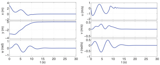
Figure 2. Trajectories of states x, y, $\psi$, u, v and r.

4.2. Comparison of Convergence Rate

To demonstrate that the control scheme in this paper has the faster convergence rate than that of first method in [12], especially near the origin, in the comparisons, we choose the initial value as ${[x\left(0\right),y\left(0\right),\psi \left(0\right),u\left(0\right),v\left(0\right),r\left(0\right)]}^T={[0.3,-0.3,0,0,0,0]}^T$.

Figure 3 shows that the trajectory of a key stabilizing variable ${\vartheta }_2$, which converges to zero in 10 s, is much faster than the method in [12]. The convergence is especially much faster near the origin due to the fractional power control law that overcomes the effect of high order nonlinear dynamics. Figure 3 and Figure 4 give three simulation results to further demonstrate the advantage of the proposed controller, wherein the positions and angle x, y and $\psi$ converge to zero in 30 s in our case, while oscillations and slower convergence are seen in the case of [12].

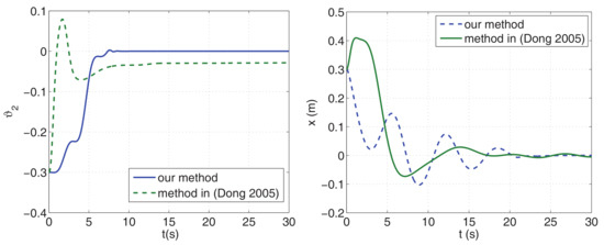
Figure 3. Comparison of the state ${\vartheta }_2$ and x-coordinate position of this paper and [12].

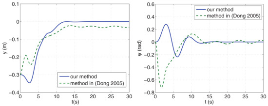
Figure 4. Comparison of the y-coordinate position and heading angel $\psi$ of this paper and [12].

To emphasize the quality of the method and the results obtained in the paper, we define a quantitative metric E as speed performance index:

$$E={(u^2+v^2+r^2)}^{\frac{1}{4}}.$$

and a quantitative metric W as states error performance index:

$$V={(x^2+y^2+{\psi }^2+u^2+v^2+r^2)}^{\frac{1}{4}}.$$

Figure 5 shows that the convergence rates of both speed performance E and states error performance W are faster with our method. It is worth mentioning that the reason we choose the order as ${\displaystyle \frac{1}{4}}$ is to show the effects of our method near the origin.

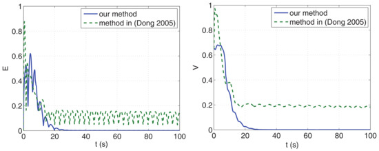
Figure 5. Comparison of the speed performance E and states convergence performance W of this paper and [12].

4.3. Comparison of Performance and Control Energy

We now look at the difference in the surge force and yaw torque of the present method and [12], shown in Figure 6. It is clearly seen that the maximum values of $|{\tau }_u|$ and $|{\tau }_r|$ in our method are smaller than [12]. It means that we can achieve a better performance with smaller control effort or energy cost. To be specific, consider the following energy cost, $J={\int }_0^t\left|\right|{\tau }_u\left(s\right),{\tau }_r\left(s\right){\left|\right|}_{2}ds$, and the accumulated error performance index, $Q={\int }_0^t{\left|\right|x\left(s\right),y\left(s\right),\psi \left(s\right),u\left(s\right),v\left(s\right),r\left(s\right)\left|\right|}_{2}ds$. We show the energy cost and performance index respectively in Figure 7, from which we can see that both the energy consumption and the accumulated error in our case are less than one third of that of [12].

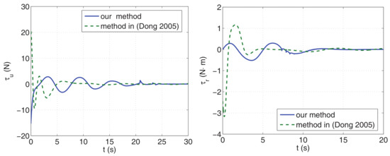
Figure 6. Comparison of surge force ${\tau }_u$ and yaw torque ${\tau }_r$ of this paper and [12].

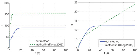
Figure 7. Comparison of energy consumption J and performance Q of this paper and [12].

5. Conclusions and Future Work

In this paper, a continuous control method is proposed for stabilization of USVs with off-diagonal inertia and damping matrices. Based on a global diffeomorphism transformation, a continuous control law is presented, which is then extended to yield a fractional power control law to increase the convergence rate of the system near the origin. Then, combing the two control laws, a switching control method is proposed to guarantee global asymptotic stabilization of USVs with faster convergence rate.

Actuator saturation due to mechanical constraints may have important impact on the system transient behavior and even stability. Stabilization of USVs subject to actuator saturation is still an open problem. Energy consumption optimized stabilization control of USVs is another interesting problem to be studied in future. Moreover, applying the theory of mechanical system [27,28,29,30,31,32] to USVs control is another problem.

References

- Pettersen, K.Y.; Egeland, O. Exponential stabilization of an underactuated surface vessel. In Proceedings of the 35th IEEE Conference on Decision and Control, Kobe, Japan, 13 December 1996; Volume 1, pp. 967–972. [Google Scholar]
- Brockett, R.W.; Millman, R.S.; Sussmann, S.J. Asymptotic stability and feedback stabilization. Differ. Geometr. Control Theory 1983, 27, 181–191. [Google Scholar]
- Oriolo, G.; Nakamura, Y. Control of mechanical systems with second-order nonholonomic constraints: Underactuated manipulators. In Proceedings of the 30th IEEE Conference on Decision and Control, Brighton, UK, 11–13 December 1991; pp. 2398–2403. [Google Scholar]
- Reyhanoglu, M. Control and stabilization of an underactuated surface vessel. In Proceedings of the 35th IEEE Conference on Decision and Control, Kobe, Japan, 13 December 1996; Volume 3, pp. 2371–2376. [Google Scholar]
- Pettersen, K.Y.; Fossen, T.I. Underactuated dynamic positioning of a ship-experimental results. IEEE Trans. Control Syst. Technol. 2000, 8, 856–863. [Google Scholar] [CrossRef]
- Ghommam, J.; Mnif, F.; Benali, A.; Derbel, N. Asymptotic backstepping stabilization of an underactuated surface vessel. IEEE Trans. Control Syst. Technol. 2006, 14, 1150–1157. [Google Scholar] [CrossRef]
- Ma, B.L. Global κ-exponential asymptotic stabilization of underactuated surface vessels. Syst. Control Lett. 2009, 58, 194–201. [Google Scholar] [CrossRef]
- Zhang, Z.; Wu, Y. Switching-based asymptotic stabilisation of underactuated ships with non-diagonal terms in their system matrices. IET Control Theory Appl. 2014, 9, 972–980. [Google Scholar] [CrossRef]
- Pettersen, K.Y.; Nijmeijer, H. Semi-global practical stabilization and disturbance adaptation for an underactuated ship. In Proceedings of the 39th IEEE Conference on Decision and Control, Sydney, Australia, 12–15 December 2000; Volume 3, pp. 2144–2149. [Google Scholar]
- Mazenc, F.; Pettersen, K.Y.; Nijmeijer, H. Global uniform asymptotic stabilization of an underactuated surface vessel. IEEE Trans. Autom. Control 2002, 47, 1759–1762. [Google Scholar] [CrossRef]
- Pettersen, K.Y.; Mazenc, F.; Nijmeijer, H. Global uniform asymptotic stabilization of an underactuated surface vessel: experimental results. IEEE Trans. Control Syst. Technol. 2004, 12, 891–903. [Google Scholar] [CrossRef]
- Dong, W.J.; Yi, G. Global time-varying stabilization of underactuated surface vessel. IEEE Trans. Autom. Control 2005, 50, 859–864. [Google Scholar] [CrossRef]
- Samson, C. Control of chained systems application to path following and time-varying point-stabilization of mobile robots. IEEE Trans. Autom. Control 1995, 40, 64–77. [Google Scholar] [CrossRef]
- Ma, B.L.; Xie, W.J. Global asymptotic trajectory tracking and point stabilization of asymmetric underactuated ships with non-diagonal inertia/damping matrices. Int. J. Adv. Robot. Syst. 2013, 10, 336. [Google Scholar]
- Zhang, Z.; Wu, Y. Further results on global stabilisation and tracking control for underactuated surface vessels with non-diagonal inertia and damping matrices. Int. J. Control 2015, 88, 1679–1692. [Google Scholar] [CrossRef]
- Xie, W.J.; Ma, B.L. Robust global uniform asymptotic stabilization of underactuated surface vessels with unknown model parameters. Int. J. Robust Nonlinear Control 2015, 25, 1037–1050. [Google Scholar] [CrossRef]
- Qian, C.; Lin, W. A continuous feedback approach to global strong stabilization of nonlinear systems. IEEE Trans. Autom. Control 2001, 46, 1061–1079. [Google Scholar] [CrossRef]
- Wang, Z.; Li, S.H.; Fei, S. Finite-time tracking control of a nonholonomic mobile robot. Asian J. Control 2009, 11, 344–357. [Google Scholar] [CrossRef]
- Li, S.H.; Ding, S.H.; Tian, Y. A finite-time state feedback stabilization method for a class of second order nonlinear systems. Acta Autom. Sin. 2007, 33, 101. [Google Scholar] [CrossRef]
- Serrano, M.E.; Scaglia, G.J.; Godoy, S.A.; Mut, V.; Ortiz, O.A. Trajectory tracking of underactuated surface vessels: A linear algebra approach. IEEE Trans. Control Syst. Technol. 2014, 22, 1103–1111. [Google Scholar] [CrossRef]
- Fossen, T.I. Marine Control Systems: Guidance, Navigation and Control of Ships, Rigs and Underwater Vehicles; Marine Cybernetics: Trondheim, Norway, 2002. [Google Scholar]
- Fossen, T.I. Guidance and Control of Ocean Vehicles; John Wiley & Sons Inc.: Hoboken, NJ, USA, 1994. [Google Scholar]
- Pettersen, K.Y. Exponential Stabilization of Underactuated Vehicles; Norwegian University of Science Technology: Trondheim, Norway, 1996. [Google Scholar]
- Do, K.D.; Pan, J. Global tracking control of underactuated ships with nonzero off-diagonal terms in their system matrices. Automatica 2005, 41, 87–95. [Google Scholar]
- Slotine, J.; Li, W. Applied Nonlinear Control; Prentice Hall: Englewood Cliffs, NJ, USA, 1991. [Google Scholar]
- Do, K.D.; Pan, J. Underactuated ships follow smooth paths with integral actions and without velocity measurements for feedback: Theory and experiments. IEEE Trans. Control Syst. Technol. 2006, 14, 308–322. [Google Scholar] [CrossRef]
- Guida, D.; Pappalardo, C.M. Forward and inverse dynamics of nonholonomic mechanical systems. Meccanica 2014, 49, 1547–1559. [Google Scholar] [CrossRef]
- Pappalardo, C.M.; Guida, D. Use of the Adjoint Method for Controlling the Mechanical Vibrations of Nonlinear Systems. Machines 2018, 6, 19. [Google Scholar] [CrossRef]
- Pappalardo, C.M.; Guida, D. Control of nonlinear vibrations using the adjoint method. Meccanica 2017, 52, 2503–2526. [Google Scholar] [CrossRef]
- Pappalardo, C.M.; Guida, D. Adjoint-based optimization procedure for active vibration control of nonlinear mechanical systems. J. Dyn. Syst. Meas. Control 2017, 139, 081010. [Google Scholar] [CrossRef]
- Pappalardo, C.M.; Patel, M.D.; Tinsley, B.; Shabana, A.A. Contact force control in multibody pantograph/ catenary systems. Proc. Inst. Mech. Eng. Part K 2016, 230, 307–328. [Google Scholar] [CrossRef]
- Guida, D.; Pappalardo, C.M. Control design of an active suspension system for a quarter-car model with hysteresis. J. Vib. Eng. Technol. 2015, 3, 277–299. [Google Scholar]
© 2018 by the authors. Licensee MDPI, Basel, Switzerland. This article is an open access article distributed under the terms and conditions of the Creative Commons Attribution (CC BY) license (http://creativecommons.org/licenses/by/4.0/).