Article

Variable Tap-Length Algorithm with Mixed Parameter

Key Laboratory of Shenzhen Internet of Things Terminal Technology, Harbin Institute of Technology Shenzhen Graduate School, Shenzhen 518055, China
*
Author to whom correspondence should be addressed.
Appl. Sci. 2018, 8(6), 939; https://doi.org/10.3390/app8060939
Submission received: 23 April 2018 / Revised: 29 May 2018 / Accepted: 4 June 2018 / Published: 6 June 2018
(This article belongs to the Section Acoustics and Vibrations)

Abstract

:

Featured Application

The method can be applied to active noise control (ANC). As all actual environments are unknown, the tap-length considerably influences ANC. The proposed algorithm can determine the optimal tap-length to optimize computation time and avoid the under-modeling problem. The effect of noise reduction can be improved to a certain extent.

Abstract

Convergence speed and steady-state performance are important factors to estimate the variable tap-length algorithm. The step-size of tap-length (ST) and the error width considerably impact the performance of the fractional variable tap-length algorithm. A mixed fractional variable tap-length algorithm that simultaneously applies time-varying ST and error width strategies is presented in this paper. The ST and the error width are analyzed in detail. This method uses the same variable to control both aspects, so their changes are relatively consistent. The parameters have strong adaptive ability at different stages. The proposed algorithm can solve some defects of the previous algorithms, including slow convergence rate, weak steady-state performance and robustness. A novel mean square deviation (MSD) gradient experiment is performed. Experimental results show good agreement with the theoretical analysis.

1. Introduction

The adaptive algorithm involves considerable investigation into signal processing, being widely applied to diverse fields including active noise control, beamforming, and echo canceling [1,2]. The tap-length is a special parameter of the adaptive algorithm. It plays a decisive role in the performance of transient and steady-state. Too small a tap-length will cause divergence [3,4]. To avoid this situation, the tap-length is usually assigned a large value in general algorithms. Nevertheless, a large tap-length also results in a large amount of computation and poor steady-state performance. Thus, finding a method to adjust tap-length is necessary. Many researchers have proposed variable tap-length algorithms. Gu et al. [5] presented a gradient descent algorithm that adjusts tap-length according to the negative gradient direction of squared estimation error. A segmented filter algorithm [6] separated the entirety into some parts and the tap-length updated in one part based on the difference of the error in the previous part. Among these variable tap-length algorithms, the fractional variable tap-length (FT) algorithm [7] is the most favored strategy.
The step-size of tap-length (ST) is important to the performance of the FT algorithm. Large ST causes fluctuations and fast convergence speed. Conversely, small ST causes the under-modeling problem and good steady-state performance [8]. Generally, there is a tradeoff between stability and convergence speed. However, ST is usually fixed in the FT algorithm. The error width of the FT algorithm also influences convergence rate and steady-state performance. Large error width improves convergence rate but results in poor steady-state performance. Small error width causes little fluctuation but decreases convergence performance [9]. Thus, many researchers proposed time-varying strategies [10,11]. Nevertheless, these algorithms cannot avoid the interference of system error or indicate the exact parameter at the same time. More importantly, they are only concerned with either ST or error width and ignore the effect of the other parameters. Coordination of these two parameters is lacking. These algorithms cannot provide the good performance.
Algorithms in [12,13] improved a certain performance compared with algorithms in [10,11]. However, they only concerned with either ST or error width and also ignored the effect of the other one. There is no reasonable analysis or adjustment strategy for the other parameter in algorithms [12,13]. Their performance may be affected by this. Thus, a mixed variable tap-length algorithm that uses the time-varying strategies of ST and error width is proposed in this paper. The proposed algorithm combines algorithms in [12,13] and balances them reasonably. ST and error width of the proposed algorithm all have good adaptive ability. The significant difference between the proposed algorithm and the algorithms in [12,13] is the performance in high noise environment. As ST and error width can meet the corresponding values at different stages, the proposed algorithm can perform well even in the high noise environment. By using a suitable and unified strategy to control ST and error width, the proposed algorithm improves convergence rate and steady-state performance. The accurate tap-length of the proposed algorithm makes the accurate estimate of the corresponding weight coefficients. Moreover, the proposed algorithm avoids interference of the system error and provides a good level of robustness. Some experiments were performed to compare the performance.
The rest of this paper is organized as follows: Section 2 introduces the least mean square (LMS) algorithm, the influence of tap-length and the FT-LMS algorithm. The proposed mixed variable tap-length algorithm and its performance analysis are introduced in Section 3 and Section 4, respectively. The detailed simulation experiments and results are outlined in Section 5. The conclusions are summarized in Section 6.

2. Variable Tap-Length Algorithm

2.1. Least Mean Square Algorithm

The LMS algorithm is composed of an input signal X , an error signal e ( n ) , an output signal y ( n ) and a weight coefficient vector W. The full equation is as follows:
y ( n ) = W ( n ) T X
e ( n ) = ( W o p t W ( n ) ) T X + v ( n )
W ( n ) = W ( n 1 ) + μ e ( n ) X
where W o p t is the optimal weight. v ( n ) is the noise signal, and μ is the step-size. When μ =   μ = μ X T X + β , it becomes the normalized least mean square algorithm (NLMS). β is a small positive number multiplied by the unit matrix. The length of the weight coefficient vector W is the tap-length. The lengths of the optimal weight W o p t and actual weight W are L o p t and L, respectively. When the tap-length L is much smaller than L o p t , the algorithm diverges. Similarly, when the tap-length L is much larger than L o p t , we can infer from Equation (2) that e ( n ) increases as well. As the computational complexity of the LMS algorithm is proportional to the tap-length L, a large tap-length L also requires a large amount of computation. To maintain the same performance level, a smaller tap-length requires less computation. Therefore, the tap-length L is a tradeoff among stability, computation, and convergence speed.

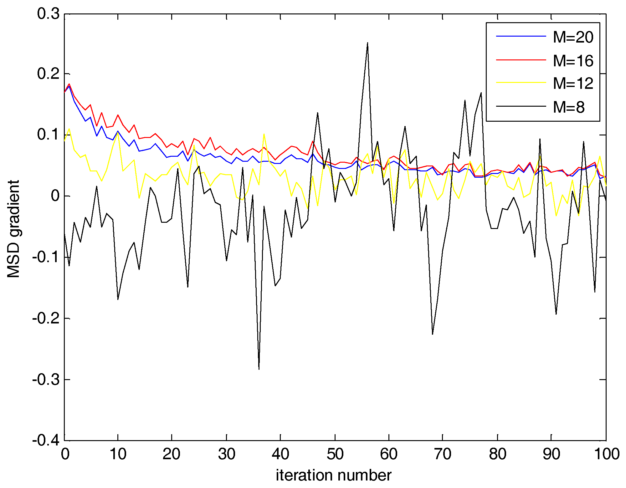
2.2. Mean Square Deviation Gradient

Next, the mean square deviation (MSD) gradient is used to discuss the effect of different tap-lengths on the algorithm. For a more intuitive comparison, we analyzed the MSD gradient first. Define p as follows:
p ( n ) = W o p t W ( n )
Taking W opt to subtract Equation (3), Equation (3) becomes as follows:
p ( n ) = p ( n 1 ) μ e ( n ) X
Using t ( n ) to replace E { p ( n 1 ) 2 } E { p ( n ) 2 } , the equation becomes as follows:
t ( n ) = E { p ( n 1 ) 2 } E { p ( n ) 2 } = E { p ( n 1 ) 2 } E { p ( n 1 ) μ X e ( n ) 2 }
Equation (6) can be simplified as follows:
t ( n ) = 2 μ E { e ( n ) 2 } 2 μ σ v 2 M μ 2 σ x 2 E { e ( n ) 2 }
where σ v 2 is the variance of the noise and σ x 2 is the variance of the input. The MSD gradient is related to tap-length and noise signal according to Equation (7). Next, an experiment was used to compare the MSD gradient of different tap-lengths.
Figure 1 plots the MSD gradient of different tap-lengths (8, 12, 16, and 20) in an identification system. This system was set up with the best tap-length of 16. The reference input was obtained by passing white Gaussian noise through a transfer system of H ( z ) = 0.35 + z 1 + z 2 . Transfer system H(z) was referenced from Yu and Cowan [7]. The length 16 of the identification system was adopted from the white Gaussian random sequence with zero-mean and unity variance. The signal-to-noise ratio (SNR) of 10 dB was obtained by adding white Gaussian interference noise. Different tap-lengths had different MSD gradient performance. In the first half of the iteration, the red line (M = 16) had the largest t ( n ) . In the latter half, although the black line (M = 8) had a fluctuating and negative MSD gradient, part of the black line was larger than the red line. This is because under-modeling appears in the black line. As its tap-length is smaller than the optimum value, the difference between its coefficient and the optimum is very large. Large and fluctuant MSD results in a large MSD gradient that is incorrect. Thus, the closer to optimum the tap-length is, the larger the amplitude of MSD gradient that will be obtained. For achieving the fastest convergence rate and the best tracking capability, the tap-length should be close to the optimum. In this case, MSD will undergo the largest decrease at each iteration and also guarantees the achievement of the lowest possible steady-state MSE [14]. Furthermore, a variable tap-length potentially gains significant computational savings. For an unknown environment, an efficient variable tap-length algorithm provides better results. The fractional variable tap-length algorithm is a favorable strategy, as explained below.

2.3. Fractional Variable Tap-Length Algorithm

Fractional variable tap-length means that the tap-length varies in the form of fraction. The sectional error refers to M length in front of the filter:
e M ( L ) = d ( n ) W L , 1 : M T X L , 1 : M
where 1 M L ; W L and X L are the weight coefficients and the input in the algorithm, respectively. W L , 1 : M and X L , 1 : M represent the first M elements of the weight coefficients and the input, respectively. The cost function of the tap-length is the square of the fragment error ξ M ( L ) = E { ( e M ( L ) ( n ) ) 2 } . Then, the algorithm outputs the most compatible L to meet the requirements.
ξ L Δ ( L ) ξ L ( L ) ε
where Δ is error width. It is a positive integer less than L. ε is a small positive integer required by the system. The minimum L satisfying Equation (9) is chosen as the optimal filter tap-length.
Tap-length is defined as an FT L f ( n ) and the iterative procedure of FT is:
L f ( n + 1 ) = ( L f ( n ) α ) γ ( n ) * [ ( e L ( n ) ( L ( n ) ) ( n ) ) 2 ( e L ( n ) Δ ( L ( n ) ) ( n ) ) 2 ]
where α is a positive leakage parameter. Its function is to avoid the problem that the tap-length is much larger than the optimal value. γ ( n ) is the step-size of tap-length (ST). It is fixed in FT algorithm. When the cumulative change of the fractional tap-length exceeds a certain value, the tap-length updates as:
L ( n + 1 ) = { L f ( n )     i f | L ( n ) L f ( n ) | > δ L ( n )       o t h e r s  
where represents the nearest integer to L f ( n ) , and δ is a small integer threshold. The weight vector values in the FT algorithm are updated as follows:
W L ( n ) ( n + 1 ) = W L ( n ) ( n ) + μ e L ( n ) ( L ( n ) ) ( n ) X L ( n )
where W L ( n ) , e L ( n ) ( L ( n ) ) , and X L ( n ) represent the weight vector, error, and the input vector, respectively. μ is the normalized step-size. It can be calculated from μ X L ( n ) T X L ( n ) + β ; μ is step-size. β is the regularization factor. It is a small positive number multiplied by the unit matrix.

3. Mixed Parameter Fractional Variable Tap-Length Algorithm

Equation (10) is the updating equation of tap-length in the transient state. As α is a small positive leakage parameter, the core method to increase or decrease the tap-length is γ [ ( e L ( n ) ( L ( n ) ) ( n ) ) 2 ( e L ( n ) Δ ( L ( n ) ) ( n ) ) 2 ] . A large value of the core part is needed to quickly change the tap-length. Thus, large ST γ and error width Δ are required to increase the convergence speed of tap-length in the transient state. In the steady-state, the updating equation of tap-length can be expressed as follows [8]:
L f ( ) = L o p t + Δ α σ x 2 σ c 2 Δ μ σ v 2 ( 2 μ ) L o p t σ x 2 σ c 2
where σ x 2 , σ v 2 are the variances of the input signal and noise signal, respectively. σ c 2 is the variance of the tail elements of the optimal weight W o p t . For the determined noise signal, a small ST and error width are needed to eliminate the last three items in the steady-state. Thus, small ST and error width allow tap-length to avoid the large fluctuations in the steady-state.
From the above, we determined that ST and error width have similar trends. In the beginning, ST and error width should be large to increase convergence speed and avoid the under-modeling problem. In the steady-state, small ST and error width are needed to improve steady-state performance and avoid overestimation of tap-length. In other words, to improve performance, the FT algorithm should simultaneously have the same time-varying strategies of ST and error width. Therefore, a novel method which adjusts ST and error width based on the fragment-full error (FE) is proposed in this study. The proposed algorithm reasonably combines ST and error width so that they coordinate and cooperate with each other. The complete iteration formula is:
F E ( n ) = ( e L ( n ) ( L ( n ) ) ( n ) ) 2 ( e L ( n ) Δ ( L ( n ) ) ( n ) ) 2
q 1 ( n ) = λ q 1 ( n 1 ) + ( 1 λ ) | F E ( n ) |
q 2 ( n ) = λ q 2 ( n 1 ) + ( 1 λ ) F E ( n )
γ ( n ) = ρ 1 q 1 ( n )
Δ ( n ) = min ( Δ m a x , ρ 2 | q 2 ( n ) | )
where q 1 ( 0 ) and q 2 ( 0 ) are zero. λ is a smoothing parameter and should be close to 1. ρ 1 and ρ 2 are the factors and their values can be referenced in Section 4. As the changing trends of ST and error width are the same, we used the same variable FE to make their changes consistent. Full error and fragment error all contain the noise signal. Subtracting them to obtain FE can eliminate the influence of the noise signal. In other words, FE is noise-free. Thus, FE reflects the state accurately and avoids external interference. Once the tap-length is far from the optimum, FE will be large. In the steady state, FE is small. Thus, FE acts as an effective method to adjust ST and error width. In the initial stage, a large FE brings a large ST and error width to avoid the suboptimal value of tap-length and improve the convergence speed. In the steady-state, a small FE produces a corresponding ST and error width to avoid fluctuation and improve the steady-state performance. We also add the restricted function introduced by Han et al. [13] into the proposed algorithm.
ζ ( n ) = C * ( ( e L ( n ) ( L ( n ) ) ( n ) ) 2 ( e L ( n ) Δ ( L ( n ) ) ( n ) ) 2 ) [ 1 + ( ( e L ( n ) ( L ( n ) ) ( n ) ) 2 ( e L ( n ) Δ ( L ( n ) ) ( n ) ) 2 ) 2 ] 0.5
L F F ( n ) = { λ 1 ζ ( n ) + ( 1 λ 1 ) F E ( n )   if   e ( n ) e ( n ) < EST λ 2 ζ ( n ) + ( 1 λ 2 ) F E ( n )           else
L f ( n + 1 ) = ( L f ( n ) α ) γ ( n ) L F F ( n )
where EST is the estimated value of MSE in deficient and sufficient tap-length situations. Its value can be obtained from previous studies [15,16]. λ 1 and λ 2 are scalar mixing parameters and satisfy 0 ≤ λ 1 < λ 2 ≤ 1.
The proposed algorithm can prevent large fluctuations which are caused by interference noise. This method stabilizes the change of the tap-length. Additionally, the restricted function allows the algorithm to adapt to the changing environments better. It also increases the robustness.
In summary, the proposed algorithm reasonably adjusts the values of ST and error width according to different states. Due to characteristics of the proposed algorithm, it can adapt to changing circumstances and return more appropriate ST and error width than other algorithms. The proposed algorithm solves many problems experienced by previous algorithms [10,11,12,13], including steady-state performance, overestimation of tap-length, adaptive ability of parameters, and convergence performance.

4. Performance Analysis

4.1. Parameter Analysis

In this section, the analysis of the proposed algorithm and general guidelines for the parameters ρ 1 and ρ 2 are exhibited. Given the information provided by Zhang et al. [8] and Han et al. [13], we deduced the reasonable values of ρ 1 and ρ 2 . Based on the analysis provided by Zhang et al. [8], the low bound and the up bound of γ are as follows:
γ l = α ( Δ k δ ) σ x 2 σ c 2 Δ μ σ v 2 ( 2 μ ) L o p t
γ u = K 2 α K 3 K 2 2 α 2 K 3 2 + 4 ( η 2 δ 2 + α 2 ) K 3 2
K 1 = Δ μ σ v 2 ( 2 μ ) L o p t
K 2 = 2 + 4 σ v 2 + 4 L o p t K 1 Δ
K 3 = 2 K 1 K 2 2 K 1 σ c 2 ( ( Δ 1 ) σ x 2 + 3 )
where σ c 2 is the variance of the tail sequence of the optimal weight. k and η are small positive numbers which can be selected according to the requirement of the steady tap-length oscillation. The values of γ l and γ u are also the guidelines of ST in all FT algorithms. These two values are coincident in different FT algorithms. The fixed γ is selected by these two parameters in FT algorithms. Then, Equation (15) can also be expressed as:
q 1 ( n ) = λ n q 1 ( 0 ) + ( 1 λ ) i = 1 n λ n i | FE ( i ) |
Taking the expectation on both sides, Equation (27) becomes:
E { q 1 ( n ) } = λ n q 1 ( 0 ) + ( 1 λ ) i = 1 n λ n i E { | FE ( i ) | } λ n q 1 ( 0 ) + ( 1 λ n ) E { | FE ( n ) | }
In the steady-state, n , as λ is smaller than one, and Equation (28) becomes:
E { q 1 { } } = E { | FE ( ) | }
The values of | FE ( n ) | and FE ( n ) can be expressed from Equation (10).
| FE ( n ) | = | e L ( n ) ( L ( n ) ) ( n ) 2 e L ( n ) Δ ( L ( n ) ) ( n ) 2 | = | L f ( n + 1 ) L f ( n ) + α γ ( n ) |
FE ( n ) = e L ( n ) ( L ( n ) ) ( n ) 2 e L ( n ) Δ ( L ( n ) ) ( n ) 2 = L f ( n + 1 ) L f ( n ) + α γ ( n )
In addition, in the steady-state, n , the mean values of Equations (30) and (31) are expressed as follows:
E { | FE ( ) | } = E { | e L ( ) ( L ( ) ) ( ) 2 e L ( ) Δ ( L ( ) ) ( ) 2 | } = E { | L f ( ) L f ( ) + α γ ( ) | } = α γ ( )
E { FE ( ) } = E { e L ( ) ( L ( ) ) ( ) 2 e L ( ) Δ ( L ( ) ) ( ) 2 } = E { L f ( ) L f ( ) + α γ ( ) } = α γ ( )
where γ ( ) is the value of ST in the steady-state. Its value is equal to the fixed γ of FT algorithm. γ ( ) and α are larger than zero. Using the bound of γ , the range of ρ 1 is obtained:
γ l E { q 1 ( ) } < ρ 1 < γ u E { q 1 ( ) }
E { q 1 ( ) } = E { | e L ( ) ( L ( ) ) ( ) 2 e L ( ) Δ ( L ( ) ) ( ) 2 | } = α γ ( )
Then, the value of ρ 2 is analyzed. When n , the steady-state Δ ( ) can be expressed as follows:
Δ ( ) = ρ 2 | E { q 2 ( ) } |
where Δ ( ) can be chosen by the requirement of the system. Too large value of Δ ( ) leads to a large tap-length bias in the steady-state. Thus, it should be a small integer value. The value of | E { q 2 ( ) } | can be deduced as follows:
q 2 ( n ) = λ n q 2 ( 0 ) + ( 1 λ ) i = 1 n λ n i FE ( i )
E { q 2 ( n ) } = λ n q 2 ( 0 ) + ( 1 λ ) i = 1 n λ n i E { FE ( i ) } λ n q 2 ( 0 ) + ( 1 λ n ) E { FE ( i ) }
| E { q 2 ( ) } | = | E { FE ( ) } |
The steady-state of q 2 can be obtained:
| E { q 2 ( ) } | = | E { e L ( ) ( L ( ) ) ( ) 2 e L ( ) Δ ( L ( ) ) ( ) 2 } | = α γ ( )
In the steady-state, the values of E { q 1 ( ) } and | E { q 2 ( ) } | are related with γ ( ) and α . The range of γ ( ) is between 0.1 and 1. However, the value of α is a few percent. It is far less than the value of γ ( ) . Thus, E { q 1 ( ) } and | E { q 2 ( ) } | are small in the steady-state. ρ 2 is expressed as follows:
ρ 2 = Δ ( ) γ ( ) α
From the above, the values of γ l and γ u are required by all FT algorithms and they should be calculated first. Then the fixed γ can be obtained. Thus, the most important parameters which are used to calculate ρ 1 and ρ 2 are γ ( ) , Δ ( ) and α . γ ( ) is equal to the fixed γ of FT algorithm. Δ ( ) and α are the general parameters for all FT algorithms. Once the general parameters that are shown in Section 5 are confirmed, the values of ρ 1 and ρ 2 will be calculated.

4.2. Performance Analysis

In the FT algorithm, a large error width causes a fluctuation and overestimation of tap-length. At the other extreme, a small error width may cause a slow convergence rate and the under-modeling problem. To begin with, a larger error width is needed to converge the tap-length to the optimal interval quickly. According to Zhang et al. [8], the optimal solution of the tap-length tends to be close to L o p t + Δ . In the steady-state, the error width should be as small as possible so that the tap-length is close to the optimal solution. Similarly, we infer that ST has the same characteristic. Thus, ST and error width should be large enough to speed up convergence in the transient state. In the steady-state, ST and error width should be reduced to improve the steady-state performance. Given these characteristics, their changing trends should be the same. The proposed algorithm uses the same FE to control ST and error width so that they are relatively consistent. The main theoretical difference between the proposed algorithm and algorithm [13] is that the proposed algorithm adds the analysis and changing strategy of the other important parameter ST. ST and error width of the proposed algorithm all have good adaptive ability. They can meet the corresponding values at different stages.
In the next step, we analyzed the characteristic of FE at different stages according to Han et al. [13]. In the transient state, W o p t , X L o p t , and P are defined as follows:
W o p t = [ W L ( n ) Δ * W ¯ L ( n ) Δ + 1 : L ( n ) * W = L ( n ) + 1 : L o p t * ]
X L o p t = [ x L ( n ) Δ * x ¯ L ( n ) Δ + 1 : L ( n ) * x = L ( n ) + 1 : L o p t * ]
P = [ W L ( n ) Δ W L ( n ) Δ * W L ( n ) Δ + 1 : L ( n ) W ¯ L ( n ) Δ + 1 : L ( n ) * 0 W = L ( n ) + 1 : L o p t * ] = [ v * v ¯ * v = * ]
Then we rewrite e L ( n ) ( L ( n ) ) ( n ) and e L ( n ) Δ ( L ( n ) ) ( n ) .
e L ( n ) ( L ( n ) ) ( n ) = x L ( n ) Δ * T v * x ¯ L ( n ) Δ + 1 : L ( n ) * T v ¯ * x = L ( n ) + 1 : L o p t * T v = * + v ( n )
e L ( n ) Δ ( L ( n ) ) ( n ) = x L ( n ) Δ * T v * + x ¯ L ( n ) Δ + 1 : L ( n ) * T W ¯ L ( n ) Δ + 1 : L ( n ) * x = L ( n ) + 1 : L o p t * T v = * + v ( n )
where v(n) is the noise signal. The expression of FE in the transient state is:
E { e L ( n ) ( L ( n ) ) ( n ) 2 e L ( n ) Δ ( L ( n ) ) ( n ) 2 } = σ x 2 E { v ¯ * T v ¯ * } σ x 2 E { W ¯ L ( n ) Δ + 1 : L ( n ) * T W ¯ L ( n ) Δ + 1 : L ( n ) * }
e L ( n ) ( L ( n ) ) ( n ) 2 and e L ( n ) Δ ( L ( n ) ) ( n ) 2 all have noise signal v(n). As we subtract the former from the latter to calculate FE, FE is immune to the noise signal. It includes two elements that are associated with the weight vector at the initial stage. The former varies, and the latter does not. Once tap-length is far from the optimum value, the former will increase. Then, FE makes ST and error width increase accordingly. Thus, convergence speed is improved in the transient stage.
Similarly, according to Han et al. [13], the estimated energy of FE in the steady-state is:
E { e L ( n ) ( L ( n ) ) ( n ) 2 e L ( n ) Δ ( L ( n ) ) ( n ) 2 } = σ x 2 E { v = * T v = * }
where v = * = W = L ( n ) Δ + 1 : L ( n ) * 0 and W L ( n ) = [ W 1 : L o p t * W ¯ L o p t + 1 : L ( n ) Δ * W = L ( n ) Δ + 1 : L ( n ) * ] in the steady-state. The expression of FE contains only one part which is associated with excessive weight in the steady-state. As excessive weight is always small, FE is also small in the steady-state. It makes a small ST and error width in the steady-state. Thus, the steady-state performance improves.
The proposed algorithm adopts the same variable FE to adjust ST and error width so that they are relatively consistent. According to the analysis of Equations (47) and (48), FE is noise-free and optimizes ST and error width at the corresponding stage. Once tap-length is far from the optimum, a large FE will bring a large ST and error width. It can avoid a suboptimal value of tap-length and improve the convergence speed. In the steady-state, small FE results in a small ST and error width to avoid fluctuation and improve the steady-state performance. The proposed algorithm equips adaptive parameters in different phases.

5. Simulations and Results

In this section, the proposed method compares with the FT algorithm [7] and other algorithms [11,12,13] via simulation. FT Algorithm 1 adopts the minimum error width and FT Algorithm 2 adopts the maximum error width. To compare the performance fairly, the experimental condition is similar to that used by Yu and Cowan [7] and Han et al. [13]. The reference input was obtained by passing white Gaussian noise through a transfer system of H ( z ) = 0.35 + z 1 + z 2 . Transfer system H ( z ) was referenced form Yu and Cowan [7]. Most experimental conditions used this transfer system. To compare these algorithms fairly, we have adopted the same systems as them. SNR of 20 dB and 0 dB were obtained by adding white Gaussian interference noise. Small-scale system and large-scale system are the typical experimental systems. However, it is difficult to compare the performance of tap-length and MSE in small-scale experimental environment. The tap-length is too small and the changing range of tap-length is very limited. The effect of contrast is not significant. Moreover, the dynamic ranges of error width and ST are relatively small. In this case, the comparison of performance cannot be very prominent. As there is rarely small-scale experimental condition except [7], it is also hard to establish a fair and universal small-scale experimental environment. Thus, the large-scale system is mainly adopted in this section. The experiment used two different unknown systems to evaluate the performance. We define:
W 1 = i = 1 150 a i z i , W 2 = i = 1 80 b i z i
W 3 = i = 1 200 c i z i , W 4 = i = 1 100 d i z i
where a i , b i , c i and d i are adopted from the white Gaussian random sequence with zero-mean and unity variance. We used W o p t = W 1 for n < 10,000 and W o p t = W 2 for 10,000     n < 20,000 in the first unknown system simulation, W o p t = W 3 for n < 10,000 and W o p t = W 4 for 10,000 n < 20,000 in the second unknown system simulation.
The general parameters ( α , μ , ε , β , δ , γ , γ ( ) , Δ ( ) and Δ m a x ) are chosen first according to the algorithm in [7] and algorithms in [11,12,13]. Every parameter is selected fairly. These general parameters have no difference for all algorithms. These general parameters are used to calculate the particular parameters in each algorithm. The detailed parameters are listed in the Table 1. The following figures were acquired from 100 and 500 independent experiments with SNR = 20 dB and SNR = 0 dB respectively.

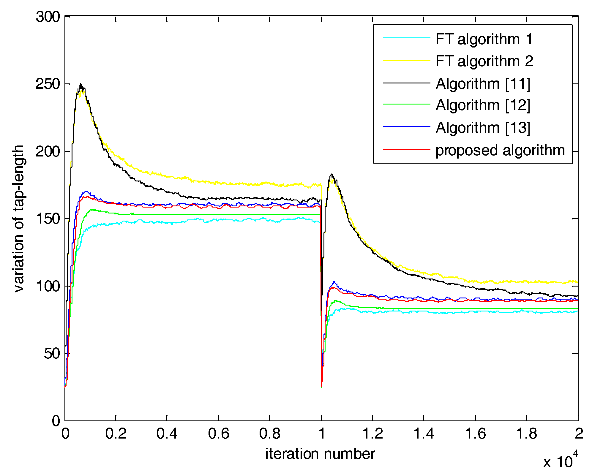
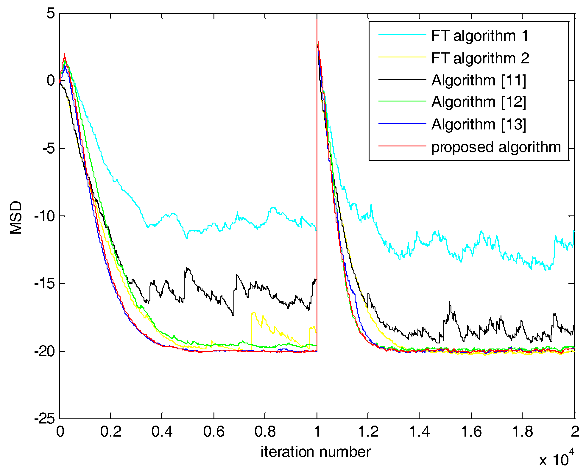
5.1. Case 1: SNR = 20 dB

We show the variation of tap-length in Figure 2 and Figure 3. As FT Algorithm 1 adopted the minimum error width, the under-modeling problem appeared. At the beginning, FT Algorithm 2 and the algorithm introduced by Mayyas et al. [11] had a large convergence rate. However, severe overestimation appeared. Tap-lengths of the algorithms introduced by Han et al. [12,13] were in the optimum range. However, the accurate ST and error width of the proposed algorithm made the corresponding tap-length estimate more accurately. The proposed algorithm maintained their advantages and mitigated their disadvantages. Before 1000, 10,500, 1300 and 10,400 iterations in Figure 2 and Figure 3, the slopes of the proposed algorithm were larger than that of the algorithm in [12]. The variation of tap-length in the proposed algorithm was relatively faster than that in the algorithm in [12]. The algorithm in [13] had a little overestimation at the beginning of iteration. The peak of the algorithm [13] was larger than that of the proposed algorithm. The performance of the proposed algorithm is the balance of these two algorithms in [12,13]. The proposed algorithm slightly improved the initial convergence speed compared with the algorithm in [12] and improved the overestimation of tap-length compared with the algorithm in [13].
Next, we compared MSD performance. The variation of tap-length correlated with MSD performance. Given the under-modeling problem in FT Algorithm 1 shown in Figure 2 and Figure 3, FT Algorithm 1 had the worst MSD performance. Similarly, lacking the varying strategy of ST or error width, MSD of FT Algorithm 2 and that of Mayyas et al. [11] were weaker than the other algorithms. Han and coworkers’ algorithms [12,13] had their respective strategies of error width or ST. However, their performance was also slightly affected by the lack of the other parameters. In the first half of Figure 4 and Figure 5, MSD of Han and coworkers’ algorithm [12] was stable at 4000 and 5000 iterations. Its MSD convergence speed was slower and its MSD was larger than the proposed algorithm. The MSD of Han and coworkers’ algorithm [13] fluctuated in the second half of Figure 5. As the proposed algorithm used strategies of ST and error width, it improved the stability and convergence performance compared with the other algorithms.

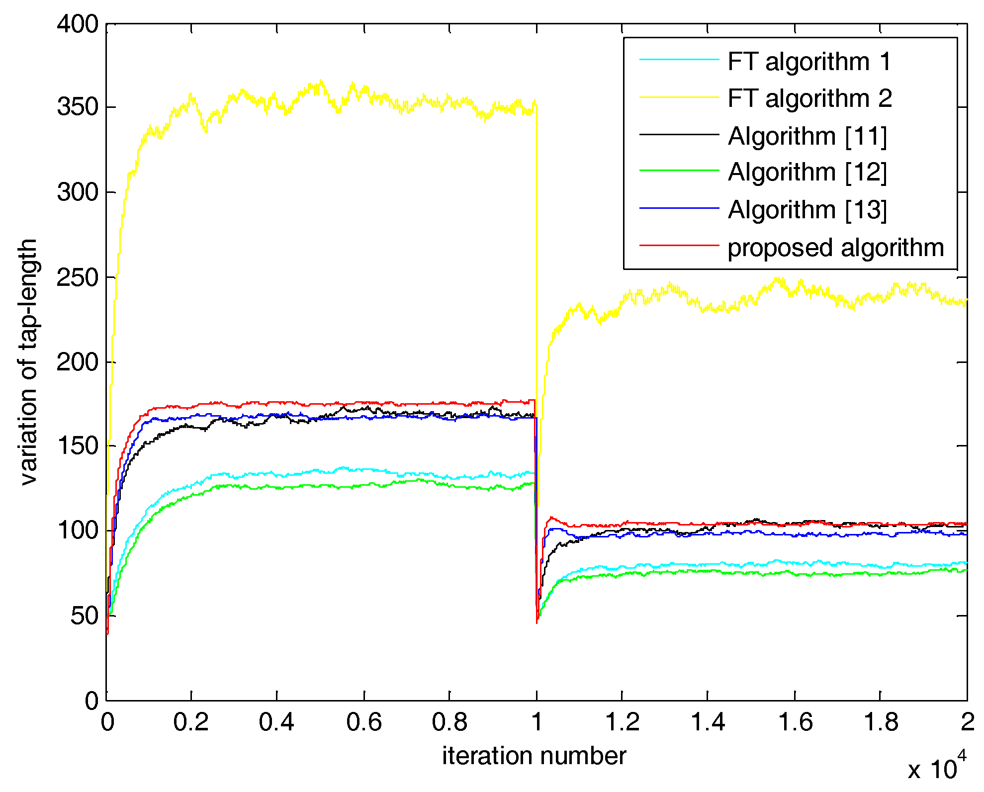
5.2. Case 2: SNR = 0 dB

The tracking abilities of Han and coworkers’ algorithm [12], FT Algorithm 1, and FT Algorithm 2 deteriorated to a certain extent in high noise condition. Under-modeling, large fluctuations and large overestimations of tap-length all appeared in these algorithms. Due to the lack of appropriate error width, the under-modeling problem appeared in Han and coworkers’ algorithm [12]. From the Figure 6 and Figure 7, the effect of error width on algorithm is greater than ST in a high noise environments. The error width acts as a decisive role in a high noise environment. These algorithms performed poorly in the SNR = 0 dB environment.
On the contrary, the algorithms of Mayyas et al. [11] and Han et al. [13], and the proposed algorithm were close to the optimum value. However, the performance of the algorithms of Mayyas et al. [11] and Han et al. [13] were also affected by the lack of reasonable choice for ST. The tap-length of the proposed algorithm converged at 1000, 11,000, 2000, and 10,500 iterations in Figure 6 and Figure 7, respectively. All other algorithms converged after these iterations. Moreover, the proposed algorithm did not fluctuate after completing convergence. The other algorithms still fluctuated. Although the environment changed, the proposed algorithm demonstrated good tracking ability and avoided large overestimations of tap-length.
In Figure 8 and Figure 9, the MSD performance of these algorithms is generally poor except the proposed algorithm. MSD performance of the proposed algorithm is low and stable. This is because accurate tap-length of the proposed algorithm made accurate estimate of the corresponding tap-coefficients. Moreover, the reasonable parameters improved the convergence and steady-state performance of the proposed algorithm. According to the analysis in Section 4, the proposed algorithm was not affected by noise. It has been confirmed by the experimental results of the high noise environment. It also has good robustness. It can adapt to changes of the environment and returns more appropriate ST and error width than the other algorithms.
Moreover, we also experimented with the MSD gradient. We chose an iteration period to compare MSD gradient. Figure 10 and Figure 11 plot the MSD gradient of different variable tap-length algorithms in SNR = 20 dB and SNR = 0 dB.
Different algorithms had different MSD gradient performance. MSD gradient is t ( n ) from Equation (5). It indicates the MSD difference between two moments in each iteration. The larger is the MSD gradient, the better is the performance that will be obtained. In Figure 10 and Figure 11, although the proposed algorithm fluctuated, its peak and bottom values were larger than those of the other algorithms. To better compare these algorithms, we calculated the mean values of the MSD gradient (Table 2). As shown in Table 2, although these variable tap-length algorithms improved MSD gradient to a certain extent, the proposed algorithm still had the largest MSD gradient. In combination with the MSD results and MSD gradient, the proposed algorithm led MSD to undergo the largest descent at each iteration. It also guaranteed the achievement of the best possible MSD performance.
The experimental results agreed with the theoretical analysis. The proposed algorithm simultaneously improved the convergence and steady-state performance.

6. Conclusions

A mixed variable tap-length algorithm which adopts the time-varying strategies of ST and error width is presented in this paper. ST and error width were analyzed in detail. The proposed method used the same variable FE to adjust ST and error width. This method ensured that their changes are relatively consistent. The proposed algorithm reasonably combined ST and error width so that they coordinated and cooperated. The convergence and steady-state performance of the proposed algorithm is improved. The overestimation problem of tap-length was also optimized. At the same time, the restricted function was added to avert large fluctuations of tap-length. The proposed algorithm can adapt to changing environments. It also increased the robustness. The experimental results agreed well with the theoretical analysis.

Author Contributions

Y.H. and M.W. conceived the research theme and designed the experiments; Y.H. and Y.L. performed the experiments; Y.H. analyzed the experimental data and wrote the manuscript; M.W. contributed materials/analysis tools and assisted to supervise the field activities. All authors read and approved the final manuscript.

Funding

This work was supported by the Shenzhen Fundamental Research Project under Grant JCYJ20170412151226061, and Grant JCYJ20170808110410773.

Acknowledgments

The authors would like to thank all the editors and reviewers for valuable feedback on this manuscript. They provided much help and suggestions in this manuscript.

Conflicts of Interest

The authors declare no conflict of interest.

References

  1. Magliacano, D.; Viscardi, M.; Dimino, I.; Concilio, A. Active vibration control by piezoceramic actuators of a car floor panel. In Proceedings of the 23rd International Congress on Sound and Vibration (ICSV), Athens, Greece, 10–14 July 2016. [Google Scholar]
  2. Qu, Y.; He, D. An adaptive remaining useful life prediction method for hybrid ceramic bearing. In Proceedings of the 2016 International Conference on Mechanics Design, Manufacturing and Automation (MDM 2016), Suzhou, China, 14–15 May 2016. [Google Scholar]
  3. Haykin, S. Adaptive Filter Theory, 3rd ed.; Prentice-Hall: Upper Saddle River, NJ, USA, 1996. [Google Scholar]
  4. Sayed, A.H. Fundamentals of Adaptive Filtering; Wiley: New York, NY, USA, 2003. [Google Scholar]
  5. Gu, Y.; Tang, K.; Cui, H. LMS algorithm with gradient descent filter length. IEEE Signal Process. Lett. 2004, 11, 305–307. [Google Scholar] [CrossRef]
  6. Riera-Palou, F.; Noras, J.M.; Cruickshank, D.G.M. Linear equalisers with dynamic and automatic length selection. Electron. Lett. 2001, 37, 1553–1554. [Google Scholar] [CrossRef]
  7. Yu, G.; Cowan, C.F.N. An LMS style variable tap-length algorithm for structure adaptation. IEEE Trans. Signal Process. 2005, 53, 2400–2407. [Google Scholar] [Green Version]
  8. Zhang, Y.; Li, N.; Chambers, J.A.; Sayed, A.H. Steady-state performance analysis of a variable tap-length LMS algorithm. IEEE Trans. Signal Process. 2008, 56, 839–845. [Google Scholar] [CrossRef] [Green Version]
  9. Li, N.; Zhang, Y.; Zhao, Y.; Hao, Y. An improved variable tap-length LMS algorithm. Signal Process. 2009, 89, 908–912. [Google Scholar] [CrossRef]
  10. Xu, D.J.; Yin, B.; Wang, W.; Zhu, W. Variable tap-length LMS algorithm based on adaptive parameters for TDL structure adaption. IEEE Signal Process. Lett. 2014, 21, 809–813. [Google Scholar]
  11. Mayyas, K.; Abuseba, H.A. A new variable length NLMS adaptive algorithm. Digit. Signal Process. 2014, 34, 82–91. [Google Scholar] [CrossRef]
  12. Han, Y.; Wang, M.; Zhao, B. Variable tap-length NLMS algorithm with adaptive parameter. IEEE Trans. Fundam. Electron. Commun. Comput. Sci. 2017, 100, 1720–1723. [Google Scholar] [CrossRef]
  13. Han, Y.; Wang, M.; Liu, M. An improved variable tap-length algorithm with adaptive parameters. Digit. Signal Process. 2018, 74, 111–118. [Google Scholar] [CrossRef]
  14. Almeida, S.J.M.D.; Bermudez, J.C.M.; Bershad, N.J.; Costa, M.H. A statistical analysis of the affine projection algorithm for unity step size and autoregressive inputs. IEEE Trans. Circ. Syst. 2005, 52, 1394–1405. [Google Scholar] [CrossRef]
  15. Mayyas, K. Performance analysis of deficient length LMS adaptive algorithm. IEEE Trans. Signal Process. 2005, 53, 2727–2734. [Google Scholar] [CrossRef]
  16. Shin, H.C.; Sayed, A.H. Mean-square performance of a family of affine projection algorithms. IEEE Trans. Signal Process. 2004, 52, 90–102. [Google Scholar] [CrossRef]
Figure 1. Mean square deviation (MSD) gradient of different tap-lengths.
Applsci 08 00939 g001
Figure 2. Tap-length variation of different algorithms in the first experimental system.
Applsci 08 00939 g002
Figure 3. Tap-length variation of different algorithms in the second experimental system.
Applsci 08 00939 g003
Figure 4. MSD of different algorithms in the first experimental system.
Applsci 08 00939 g004
Figure 5. MSD of different algorithms in the second experimental system.
Applsci 08 00939 g005
Figure 6. Tap-length variation of different algorithms in SNR = 0 dB.
Applsci 08 00939 g006
Figure 7. Tap-length variation of different algorithms in SNR = 0 dB.
Applsci 08 00939 g007
Figure 8. MSD of different algorithms in SNR = 0 dB.
Applsci 08 00939 g008
Figure 9. MSD of different algorithms in SNR = 0 dB.
Applsci 08 00939 g009
Figure 10. MSD gradient of different algorithms in SNR = 20 dB.
Applsci 08 00939 g010
Figure 11. MSD gradient of different algorithms in SNR = 0 dB.
Applsci 08 00939 g011
Table 1. Parameters of the compared algorithms.
AlgorithmSNR = 20 dBSNR = 0 dB
General α = 0.03 ,   μ = 1 ,   ε = 1 , β = 0.1 , δ = 1 , γ = 0.5 , γ ( ) = 0.5 , Δ ( ) = 1 , Δ m a x = 20 α = 0.03 , μ = 0.3 ,   ε = 1 , β = 0.1 , δ = 1 , γ = 0.5 , γ ( ) = 0.5 , Δ ( ) = 1 , Δ m a x = 50
FT Algorithm 1 γ = 0.5 , Δ = 1 γ = 0.5 ,   Δ = 1
FT Algorithm 2 γ = 0.5 ,   Δ = 20 γ = 0.5 ,   Δ = 50
Algorithm [11] γ = 0.5 , Δ m a x = 20 , Δ ( ) = 1 γ = 0.5 , Δ m a x = 50 , Δ ( ) = 1
Algorithm [12] Δ = 4 , ρ = 2 , C = 0.02 Δ = 4 ,   ρ = 2 , C = 0.02
Algorithm [13] γ = 0.5 , ρ = 16 , Δ ( ) = 1 , C = 0.5,
λ 1 = 0.9 , λ 2 = 0.95
γ = 0.5 , ρ = 16 , Δ ( ) = 1 , C = 0.5,
λ 1 = 0.9 , λ 2 = 0.95
Proposed algorithm ρ 1 = 0.01 , ρ 2 = 16 , γ ( ) = 0.5 ,
Δ ( ) = 1 , C = 0.5, λ 1 = 0.9 , λ 2 = 0.95
ρ 1 = 0.01 , ρ 2 = 16 , γ ( ) = 0.5 ,
Δ ( ) = 1 , C = 0.5, λ 1 = 0.9 , λ 2 = 0.95
Table 2. Mean value of MSD gradient in different SNR environments.
Mean ValueSNR = 20 dBSNR = 0 dB
FT Algorithm 10.29770.0701
FT Algorithm 20.23650.1259
Algorithm [11]0.23900.1244
Algorithm [12]0.36240.0700
Algorithm [13]0.36600.1613
Proposed algorithm0.38720.1774

