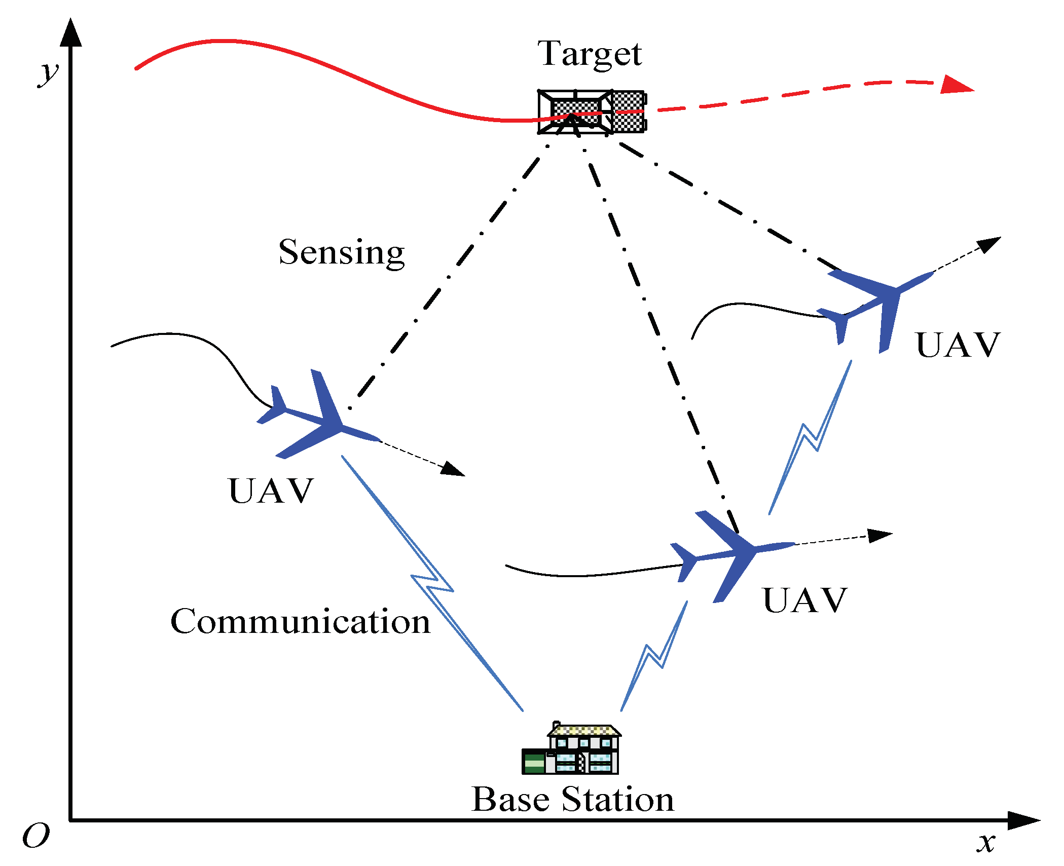
Figure 1.
The scenario where a fixed base station utilizes multi-UAVs for tracking a ground moving target.
Figure 1.
The scenario where a fixed base station utilizes multi-UAVs for tracking a ground moving target.
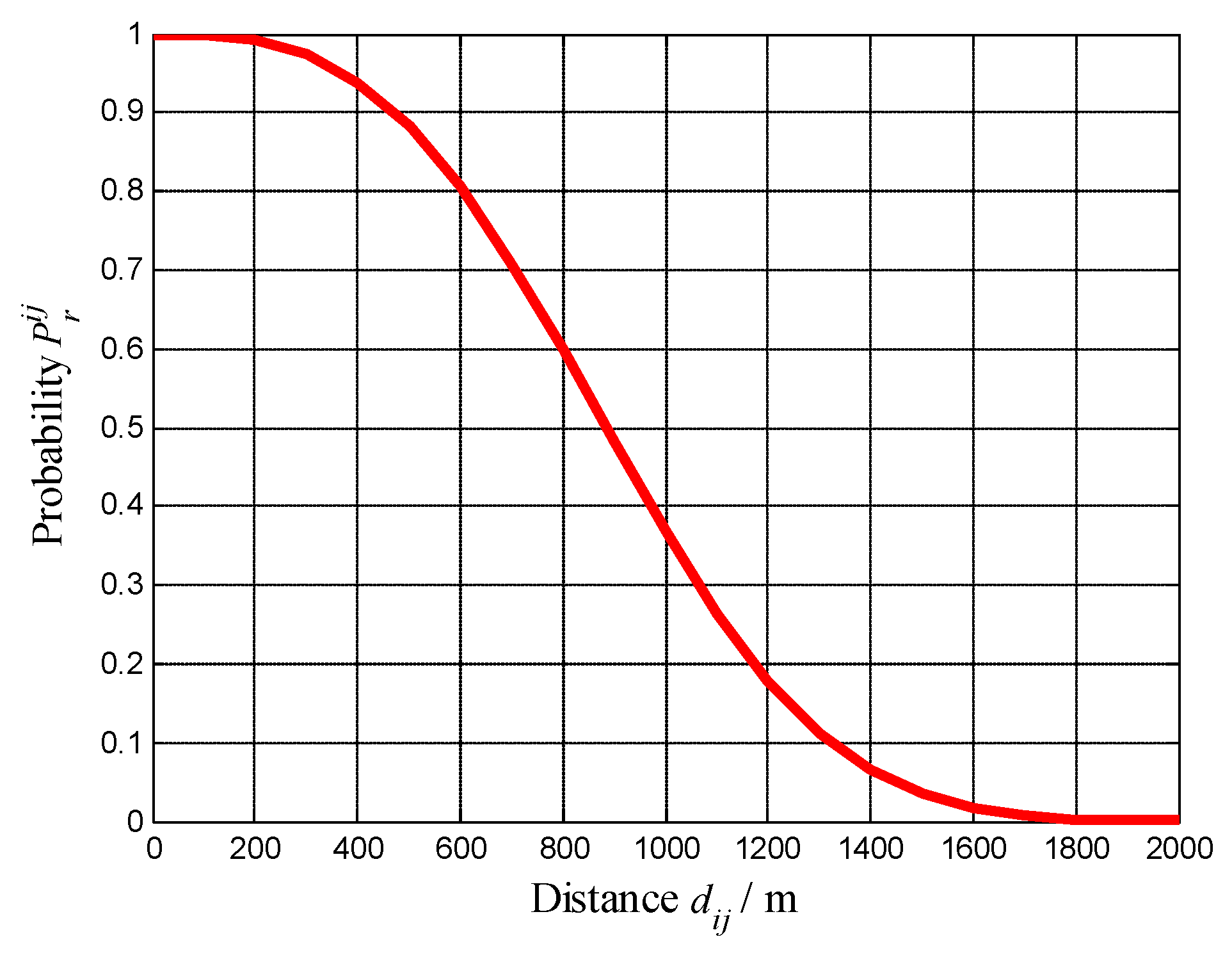
Figure 2.
The probability of a successful transmission vs. distance, as determined by Equation (11) for the parameters listed in
Table 1.
Figure 2.
The probability of a successful transmission vs. distance, as determined by Equation (11) for the parameters listed in
Table 1.
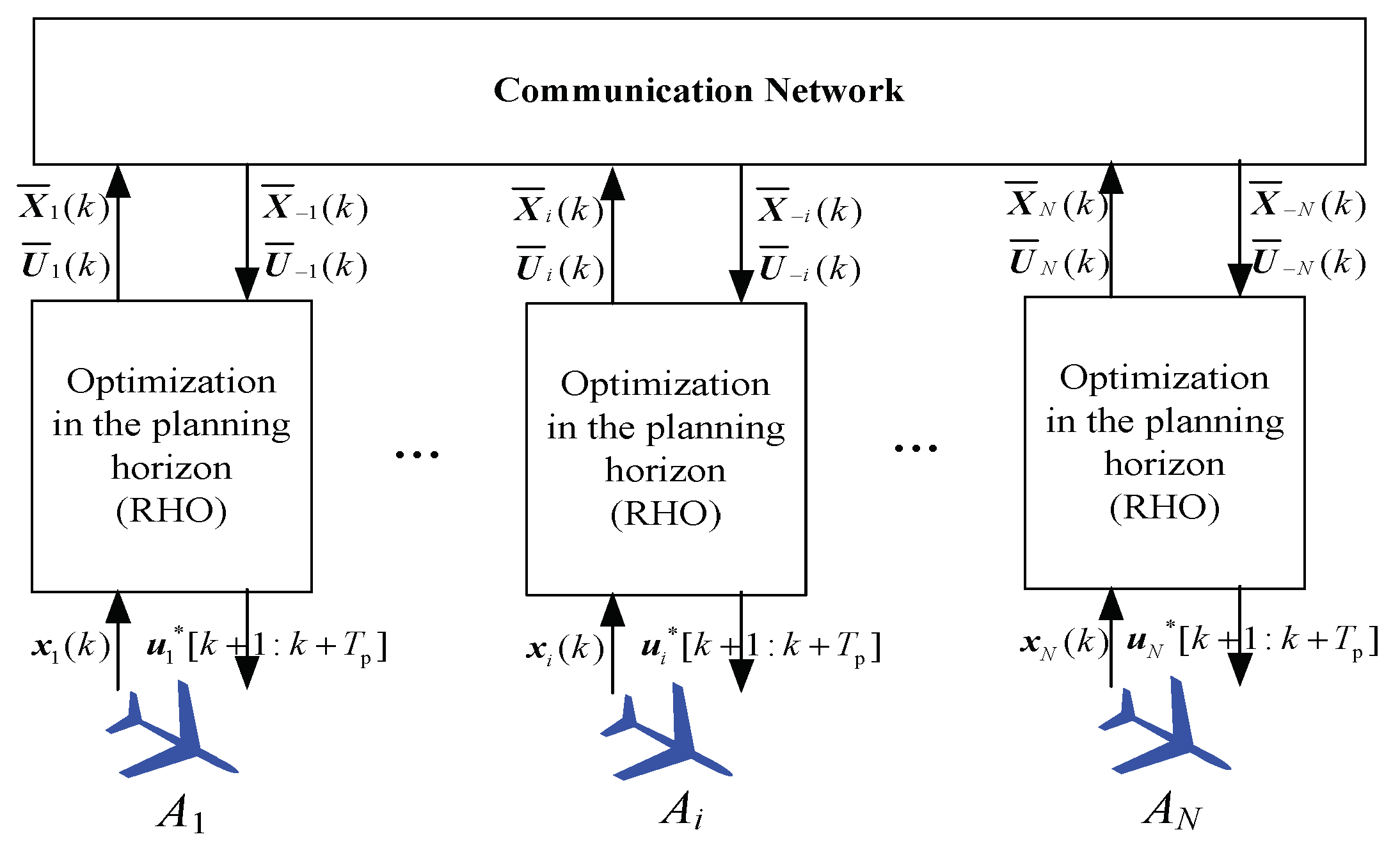
Figure 3.
Sketch of the distributed decision-making model for multiple UAV cooperative target tracking.
Figure 3.
Sketch of the distributed decision-making model for multiple UAV cooperative target tracking.
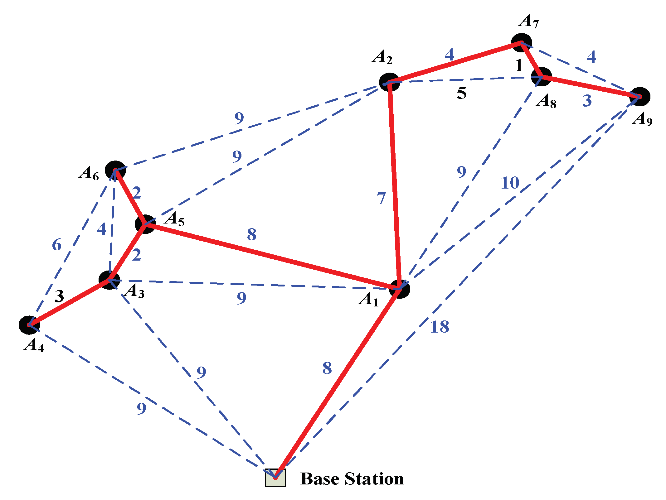
Figure 4.
Example of a communication topology and its corresponding minimum weighted spanning tree.
Figure 4.
Example of a communication topology and its corresponding minimum weighted spanning tree.
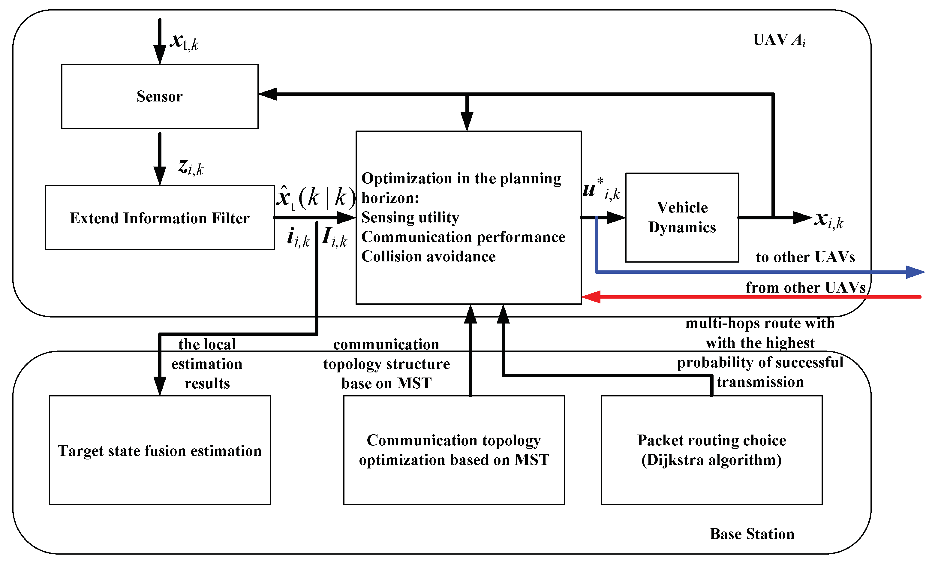
Figure 5.
Processing diagram for multi-UAVs cooperative target tracking algorithm.
Figure 5.
Processing diagram for multi-UAVs cooperative target tracking algorithm.
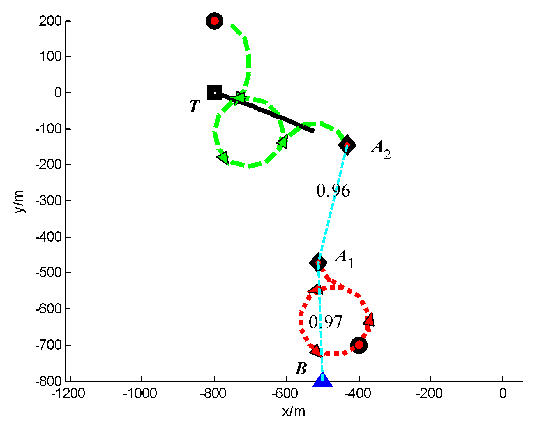
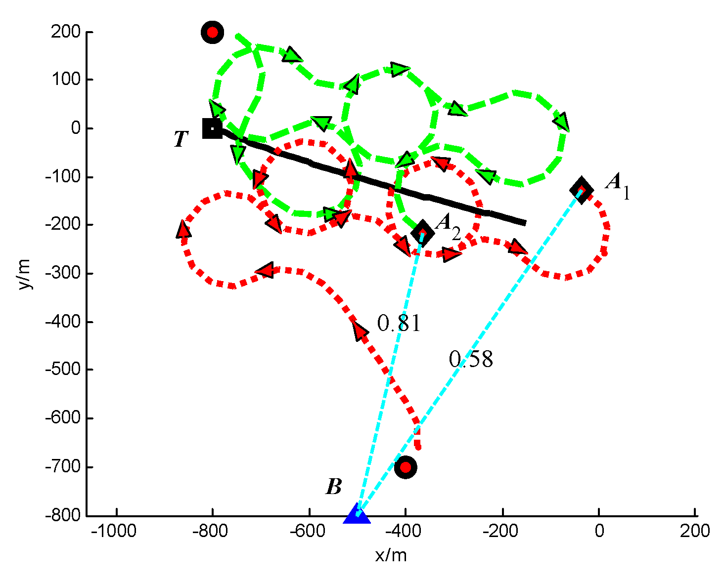
Figure 6.
Trajectories of UAVs and target at t = 30 s (Group A in Scenario 1).
Figure 6.
Trajectories of UAVs and target at t = 30 s (Group A in Scenario 1).
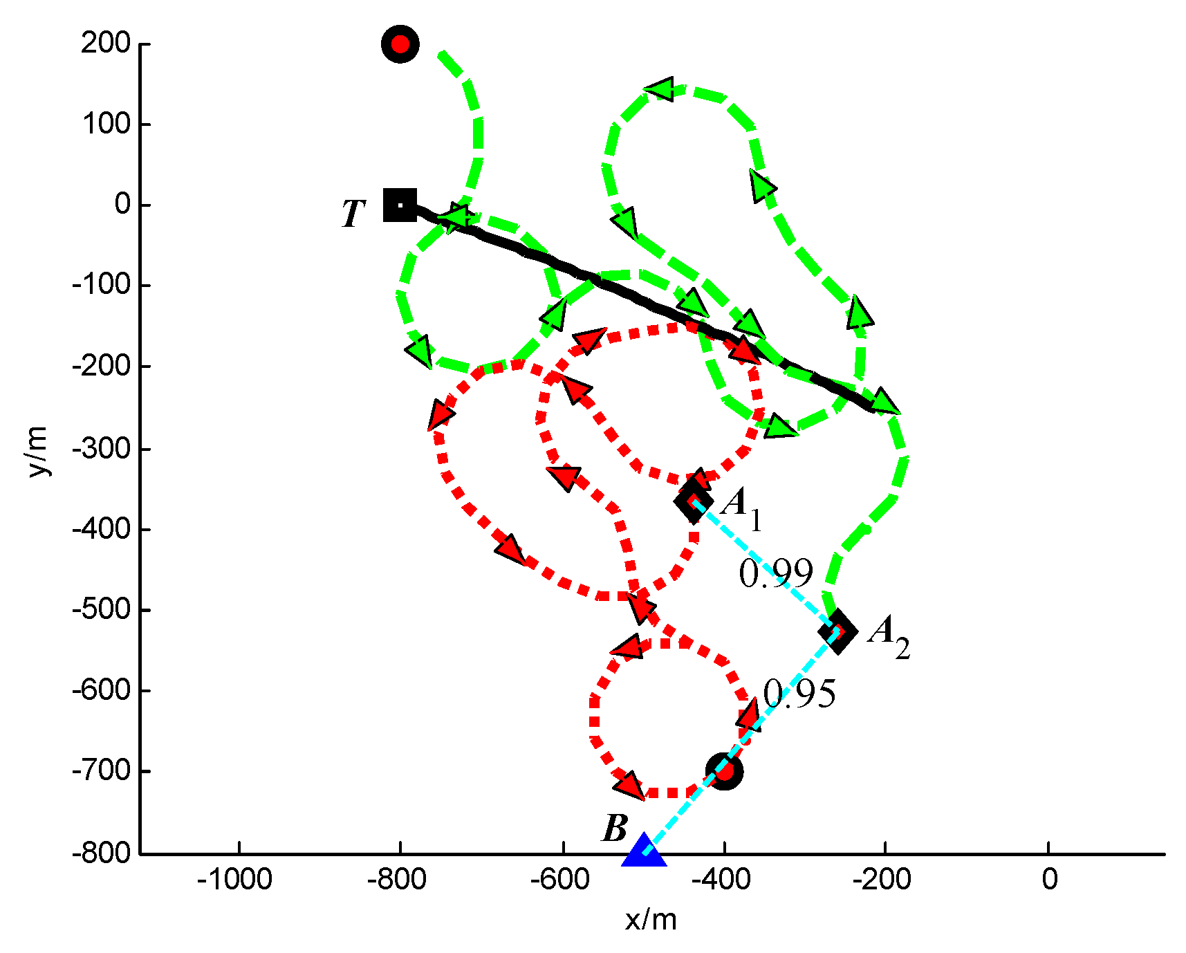
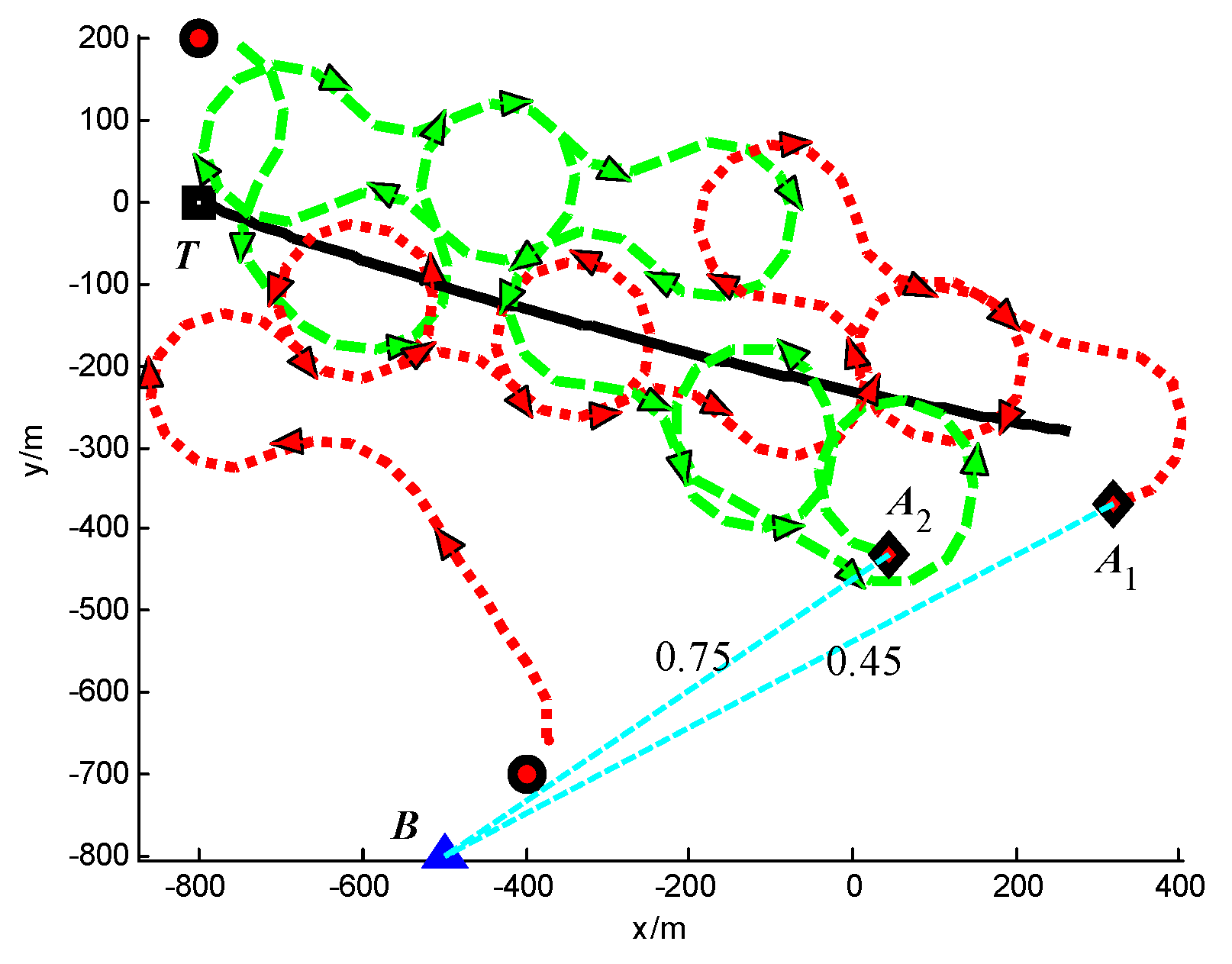
Figure 7.
Trajectories of UAVs and target at t = 64 s (Group A in Scenario 1).
Figure 7.
Trajectories of UAVs and target at t = 64 s (Group A in Scenario 1).
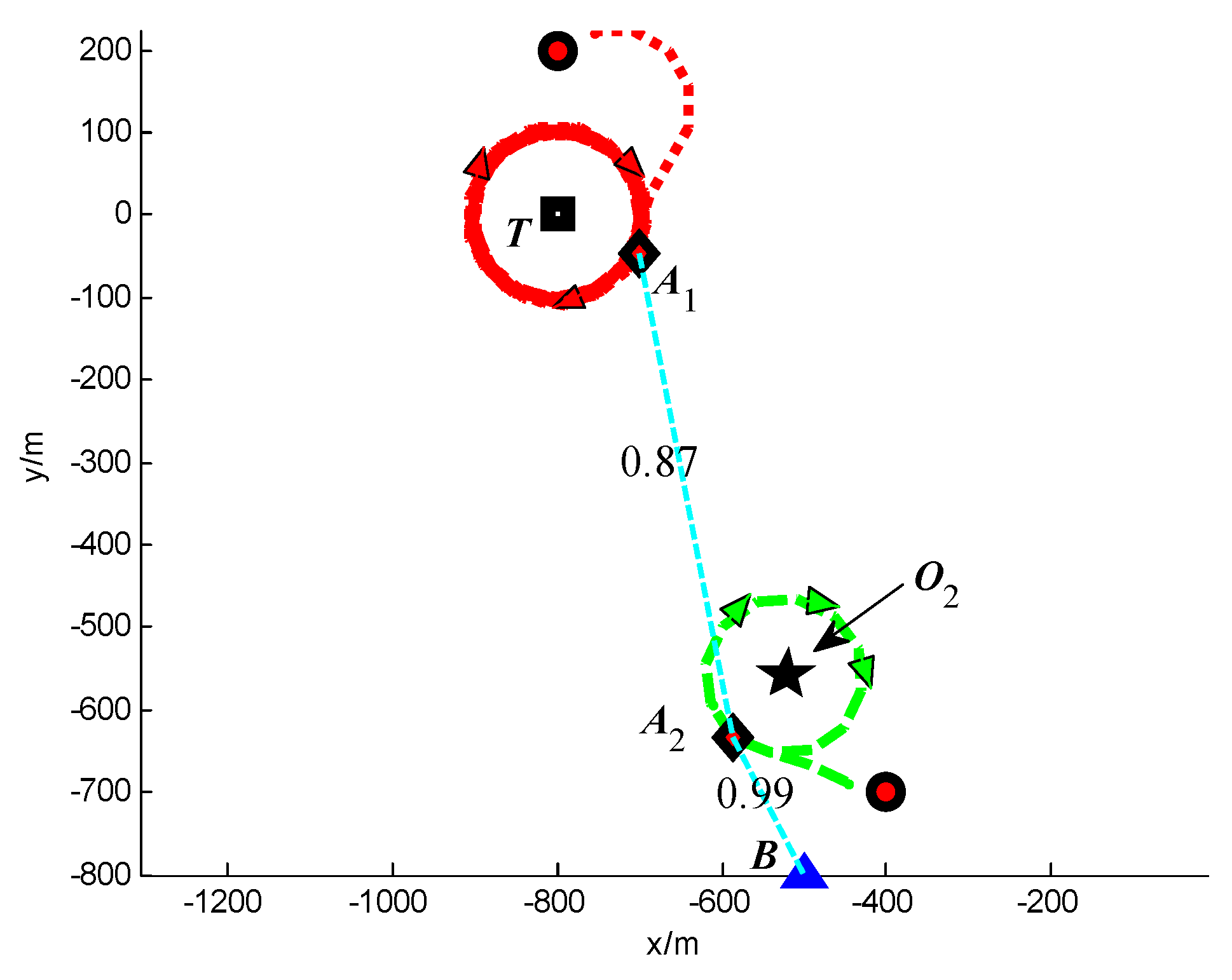
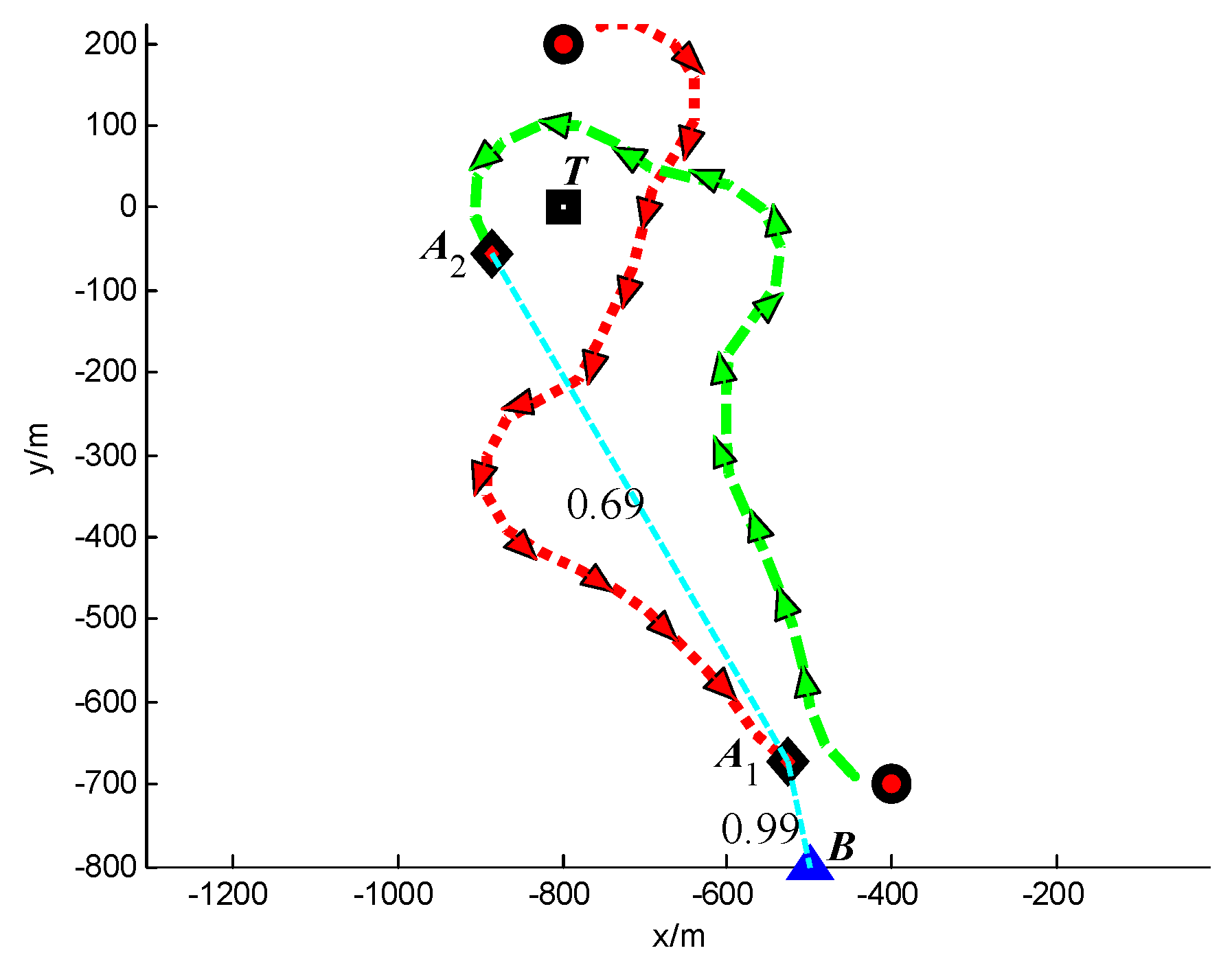
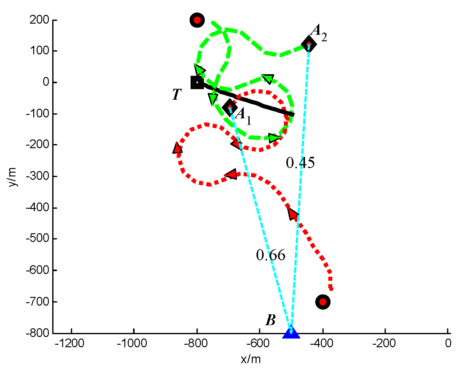
Figure 8.
Trajectories of UAVs and target at t = 100 s (Group A in Scenario 1).
Figure 8.
Trajectories of UAVs and target at t = 100 s (Group A in Scenario 1).
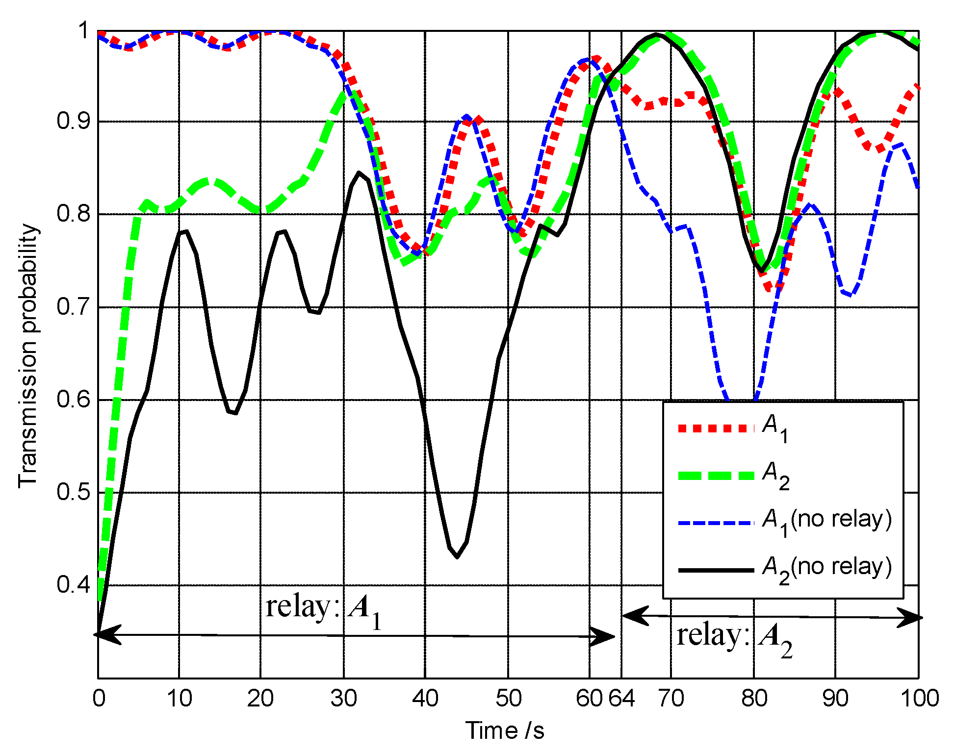
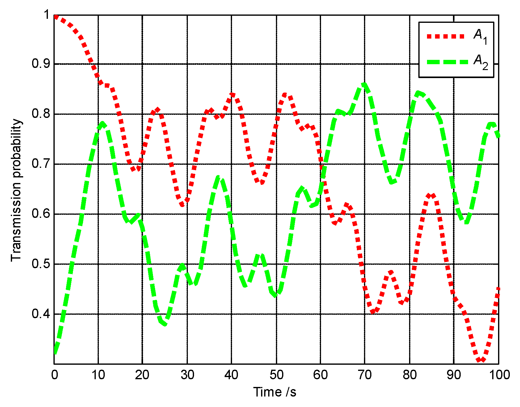
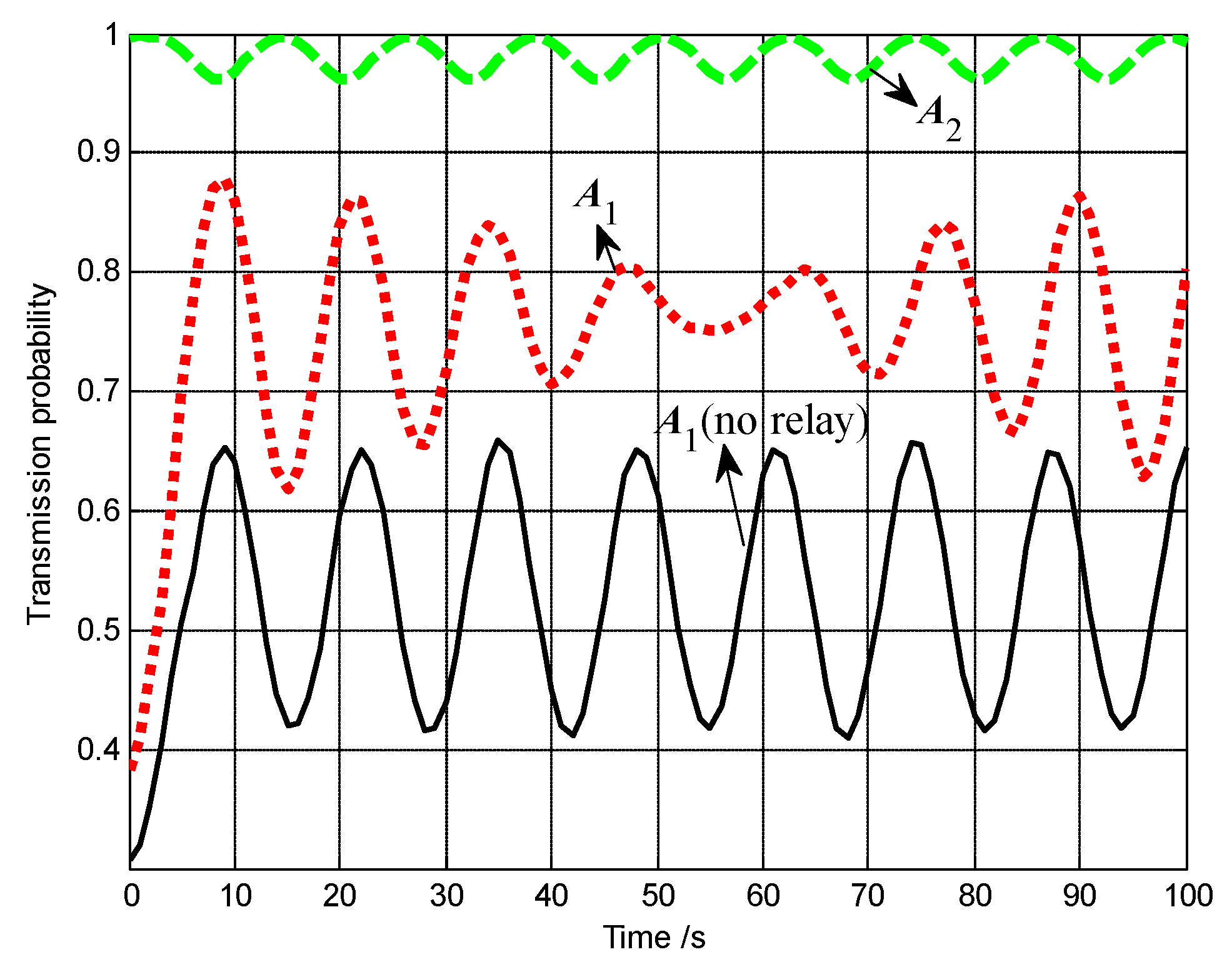
Figure 9.
The probabilities of successful transmission of A1 and A2 to base station (Group A in Scenario 1).
Figure 9.
The probabilities of successful transmission of A1 and A2 to base station (Group A in Scenario 1).
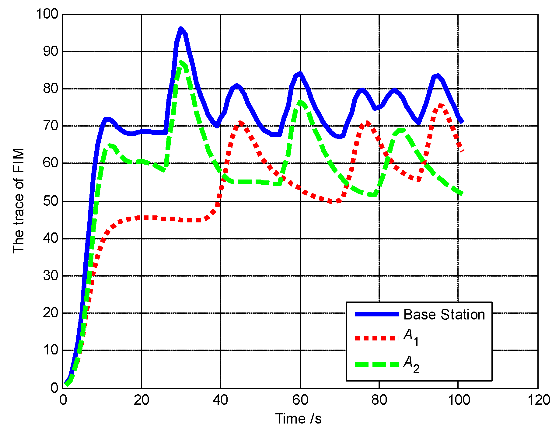
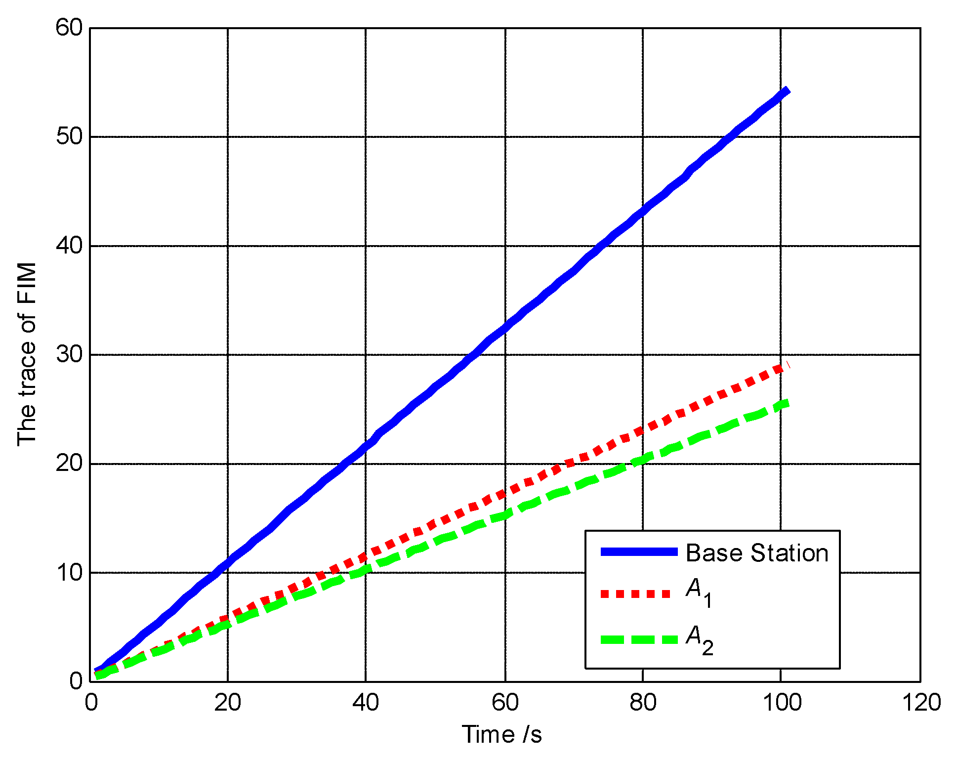
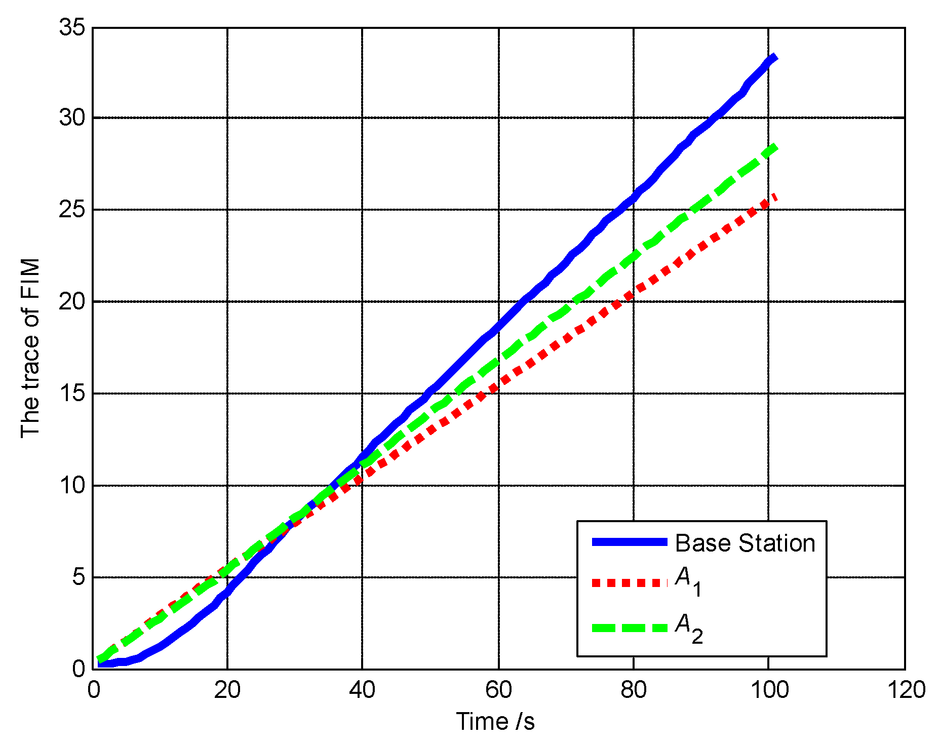
Figure 10.
The track of FIM of A1, A2 and base station (Group A in Scenario 1).
Figure 10.
The track of FIM of A1, A2 and base station (Group A in Scenario 1).
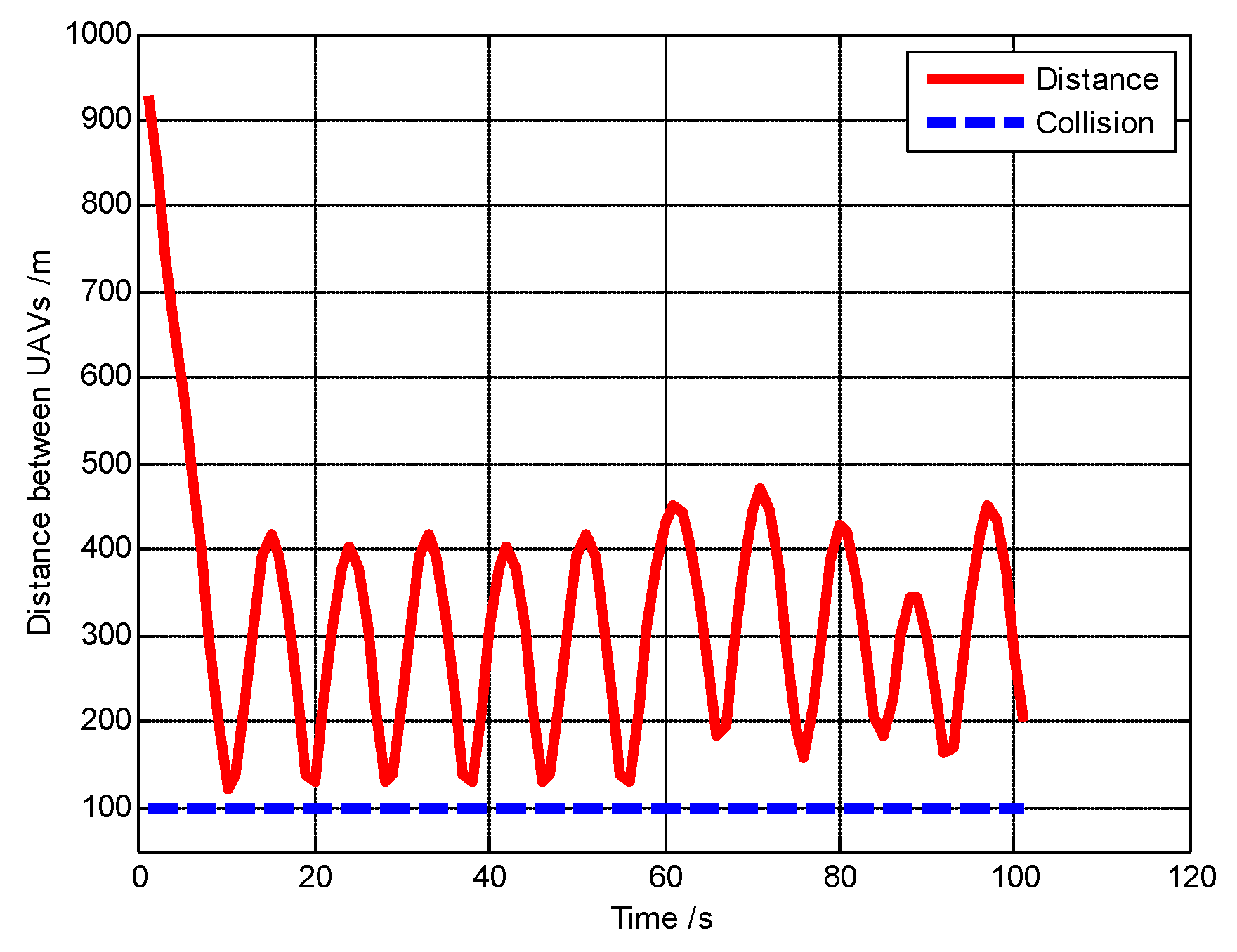
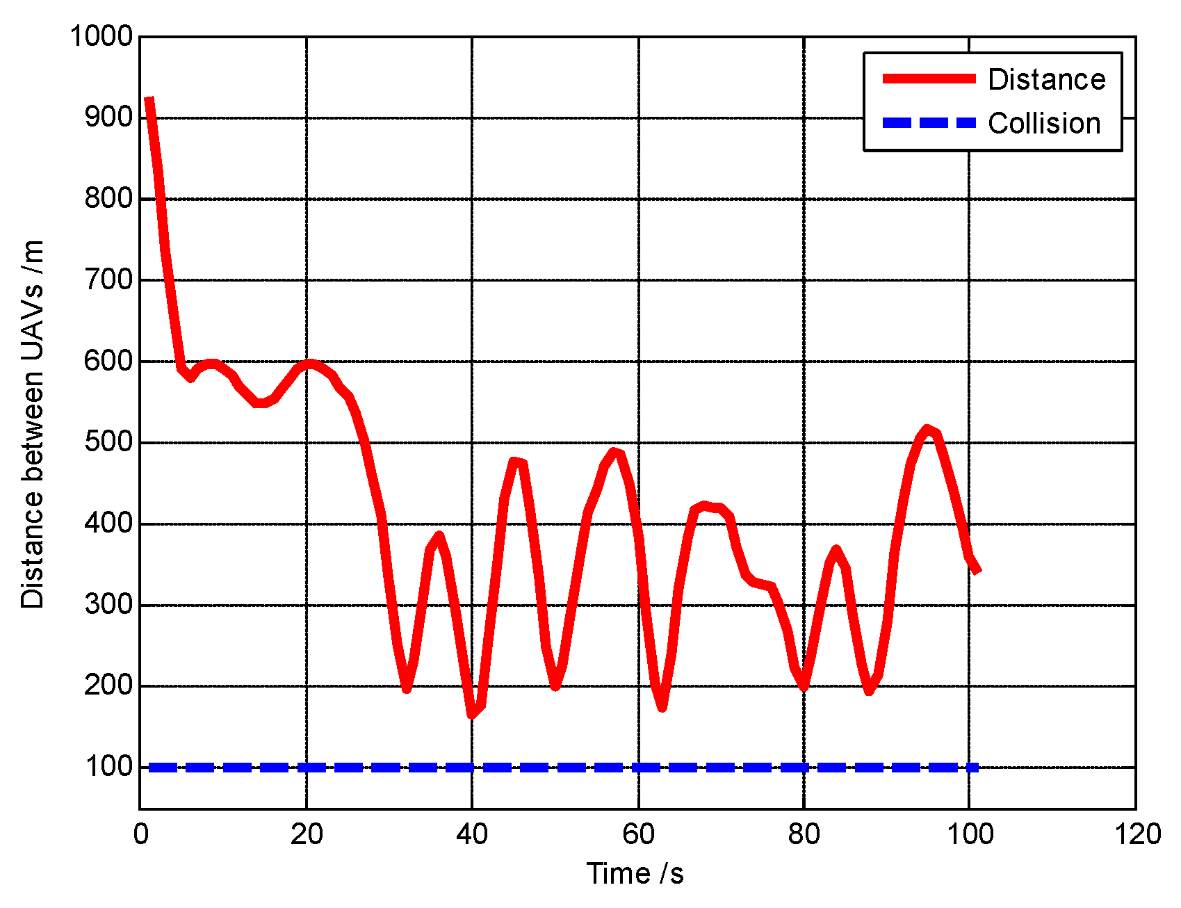
Figure 11.
The distance between the UAVs during the simulation process (Group A in Scenario 1).
Figure 11.
The distance between the UAVs during the simulation process (Group A in Scenario 1).
Figure 12.
Trajectories of UAVs and target at t = 30 s (Group B in Scenario 1).
Figure 12.
Trajectories of UAVs and target at t = 30 s (Group B in Scenario 1).
Figure 13.
Trajectories of UAVs and target at t = 64 s (Group B in Scenario 1).
Figure 13.
Trajectories of UAVs and target at t = 64 s (Group B in Scenario 1).
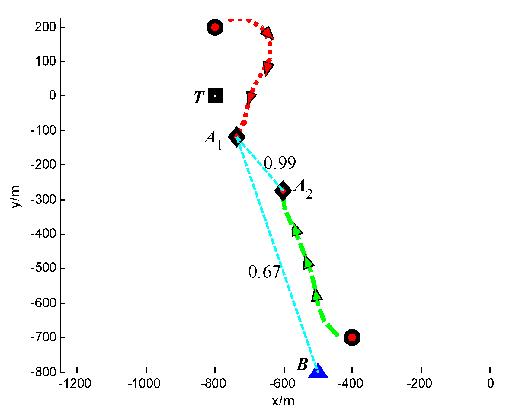
Figure 14.
Trajectories of UAVs and target at t = 100 s (Group B in Scenario 1).
Figure 14.
Trajectories of UAVs and target at t = 100 s (Group B in Scenario 1).
Figure 15.
The probabilities of successful transmission of A1 and A2 to base station (Group B in Scenario 1).
Figure 15.
The probabilities of successful transmission of A1 and A2 to base station (Group B in Scenario 1).
Figure 16.
The trace of the FIM for A1, A2 and base station (Group B in Scenario 1).
Figure 16.
The trace of the FIM for A1, A2 and base station (Group B in Scenario 1).
Figure 17.
The distance between the UAVs during the simulation process (Group B in Scenario 1).
Figure 17.
The distance between the UAVs during the simulation process (Group B in Scenario 1).
Figure 18.
Trajectories of UAVs at t = 10 s (Group A in Scenario 2).
Figure 18.
Trajectories of UAVs at t = 10 s (Group A in Scenario 2).
Figure 19.
Trajectories of UAVs at t = 100 s (Group A in Scenario 2).
Figure 19.
Trajectories of UAVs at t = 100 s (Group A in Scenario 2).
Figure 20.
The probabilities of successful transmission of A1 and A2 to base station (Group A in Scenario 2).
Figure 20.
The probabilities of successful transmission of A1 and A2 to base station (Group A in Scenario 2).
Figure 21.
The trace of the FIM for A1, A2 and base station (Group A in Scenario 2).
Figure 21.
The trace of the FIM for A1, A2 and base station (Group A in Scenario 2).
Figure 22.
Trajectories of UAVs at t = 10 s (Group B in Scenario 2).
Figure 22.
Trajectories of UAVs at t = 10 s (Group B in Scenario 2).
Figure 23.
Trajectories of UAVs at t = 20 s (Group B in Scenario 2).
Figure 23.
Trajectories of UAVs at t = 20 s (Group B in Scenario 2).
Figure 24.
Trajectories of UAVs at t = 100 s (Group B in Scenario 2).
Figure 24.
Trajectories of UAVs at t = 100 s (Group B in Scenario 2).
Figure 25.
The probabilities of successful transmission of A1 and A2 to base station (Group B in Scenario 2).
Figure 25.
The probabilities of successful transmission of A1 and A2 to base station (Group B in Scenario 2).
Figure 26.
The track of the FIM for A1, A2 and base station (Group B in Scenario 2).
Figure 26.
The track of the FIM for A1, A2 and base station (Group B in Scenario 2).
Figure 27.
Trajectories of UAVs and target at t = 10 s (Group A in Scenario 3).
Figure 27.
Trajectories of UAVs and target at t = 10 s (Group A in Scenario 3).
Figure 28.
Trajectories of UAVs and target at t = 50 s (Group A in Scenario 3).
Figure 28.
Trajectories of UAVs and target at t = 50 s (Group A in Scenario 3).
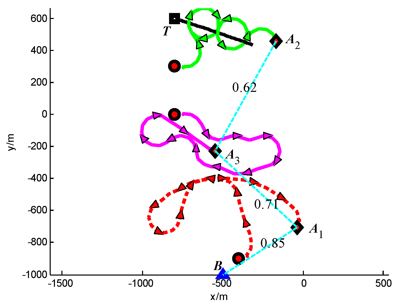
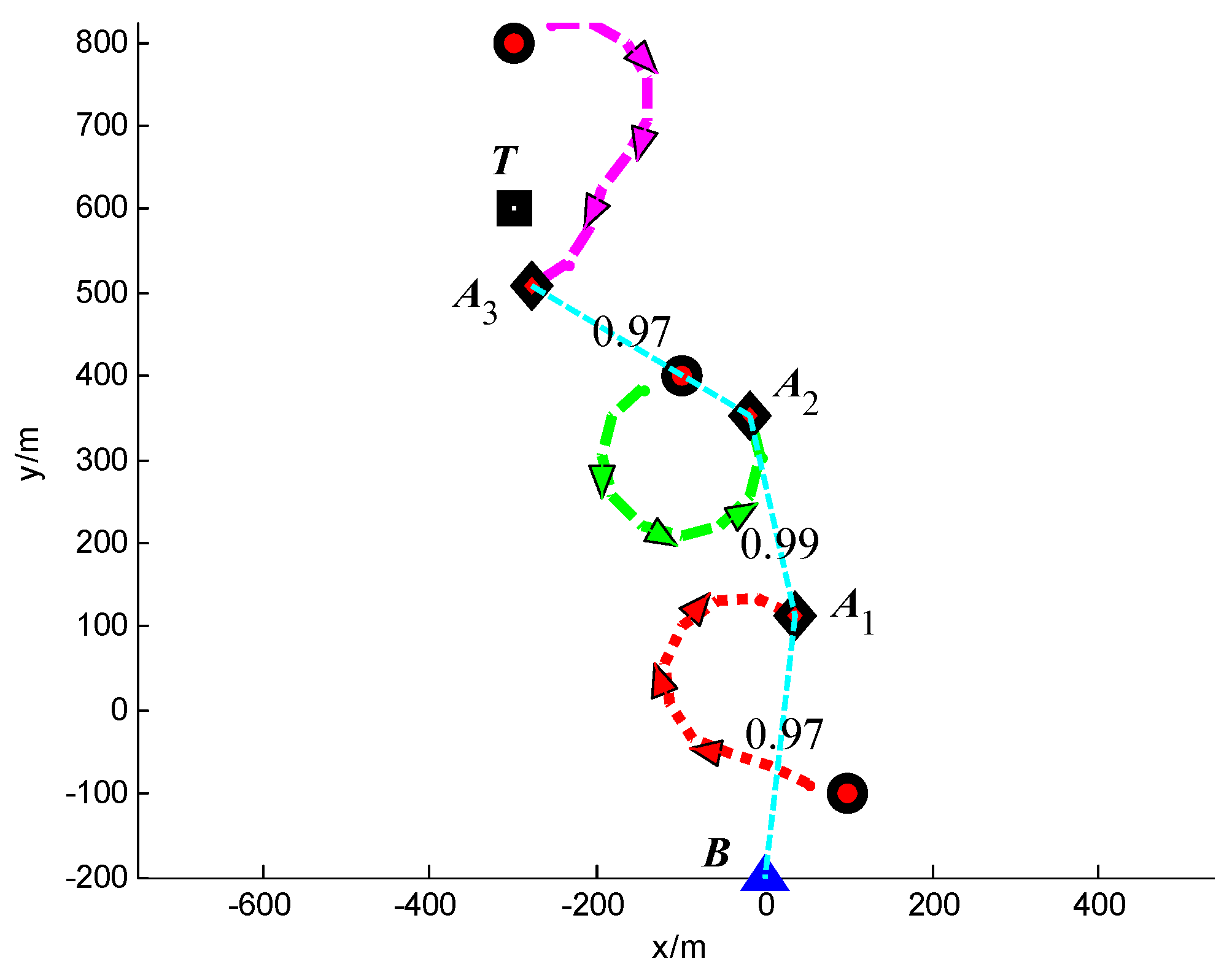
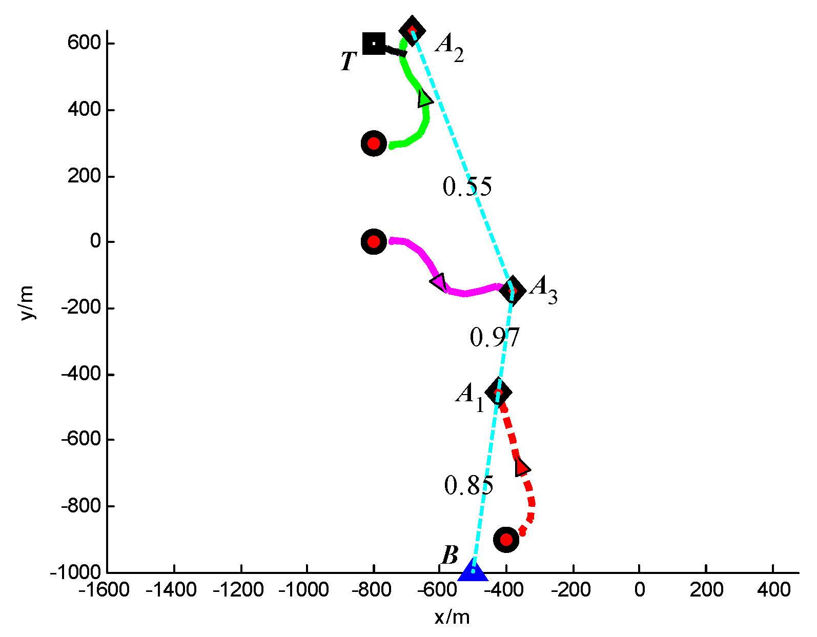
Figure 29.
Trajectories of UAVs and target at t = 100 s (Group A in Scenario 3).
Figure 29.
Trajectories of UAVs and target at t = 100 s (Group A in Scenario 3).
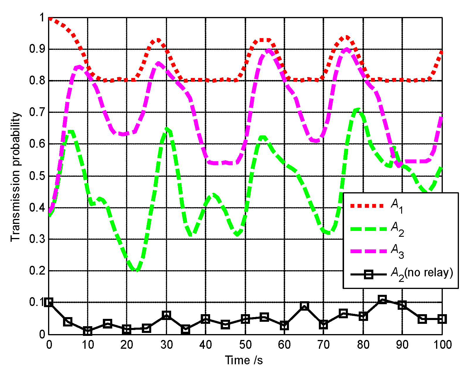
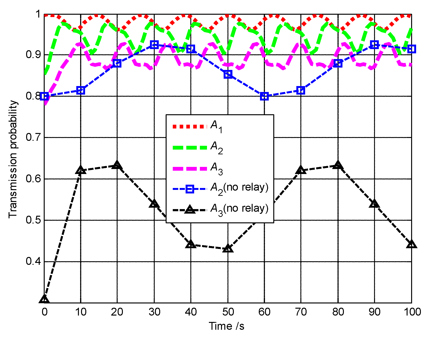
Figure 30.
The communication performances of A1, A2 and A3 (Scenario 3).
Figure 30.
The communication performances of A1, A2 and A3 (Scenario 3).
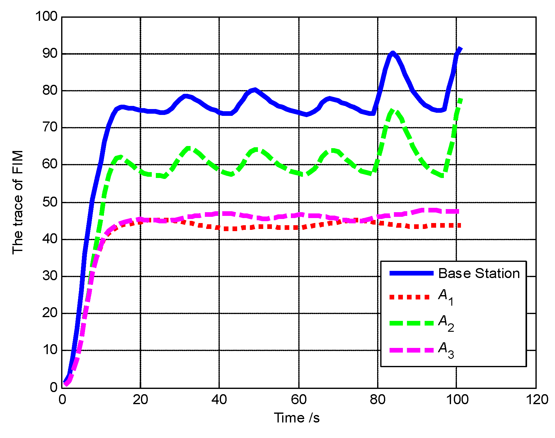
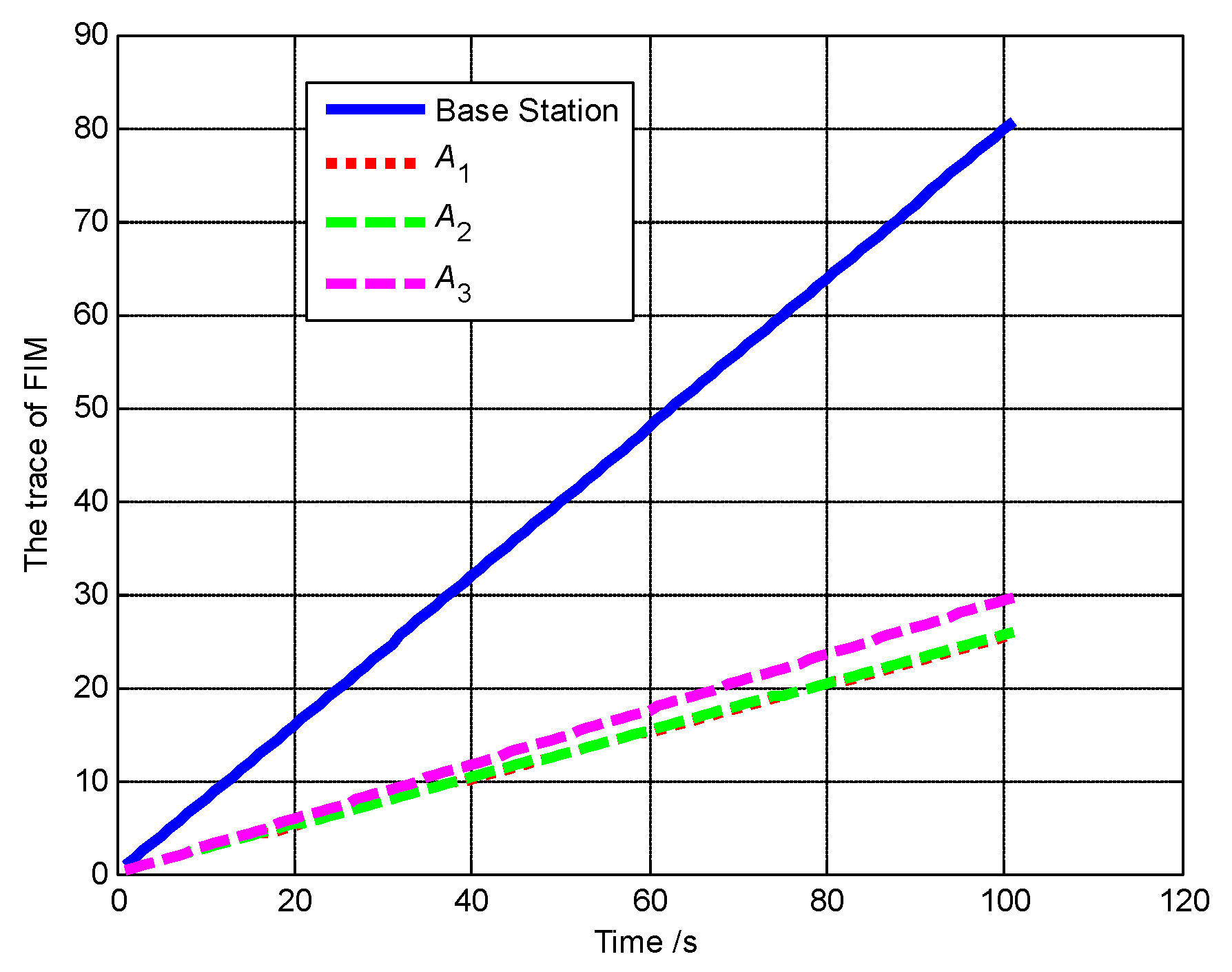
Figure 31.
The track of FIM of A1, A2, A3 and base station (Scenario 3).
Figure 31.
The track of FIM of A1, A2, A3 and base station (Scenario 3).
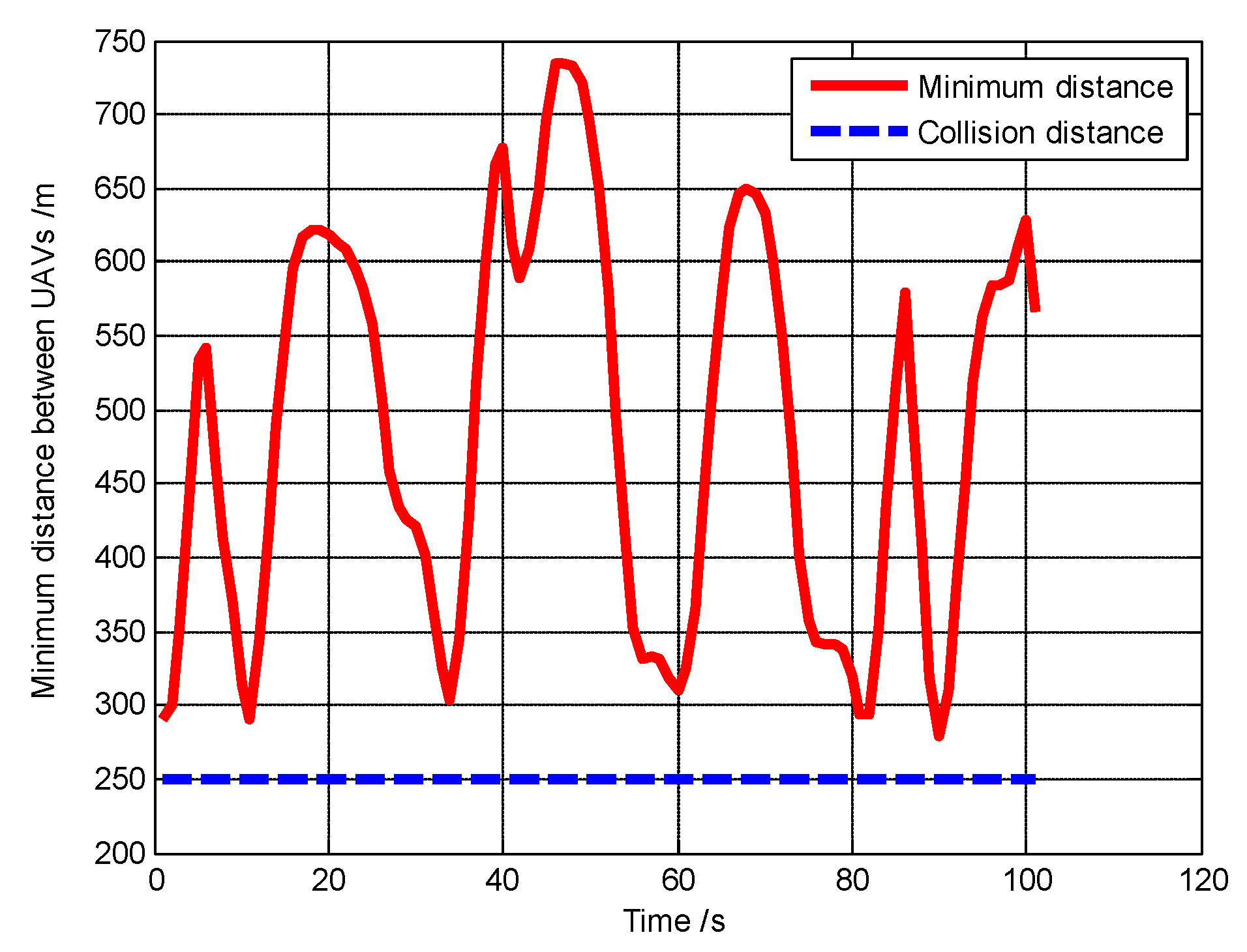
Figure 32.
The minimum distance between the UAVs during the whole simulation process (Scenario 3).
Figure 32.
The minimum distance between the UAVs during the whole simulation process (Scenario 3).
Figure 33.
Trajectories of UAVs at t = 10 s (Scenario 4).
Figure 33.
Trajectories of UAVs at t = 10 s (Scenario 4).
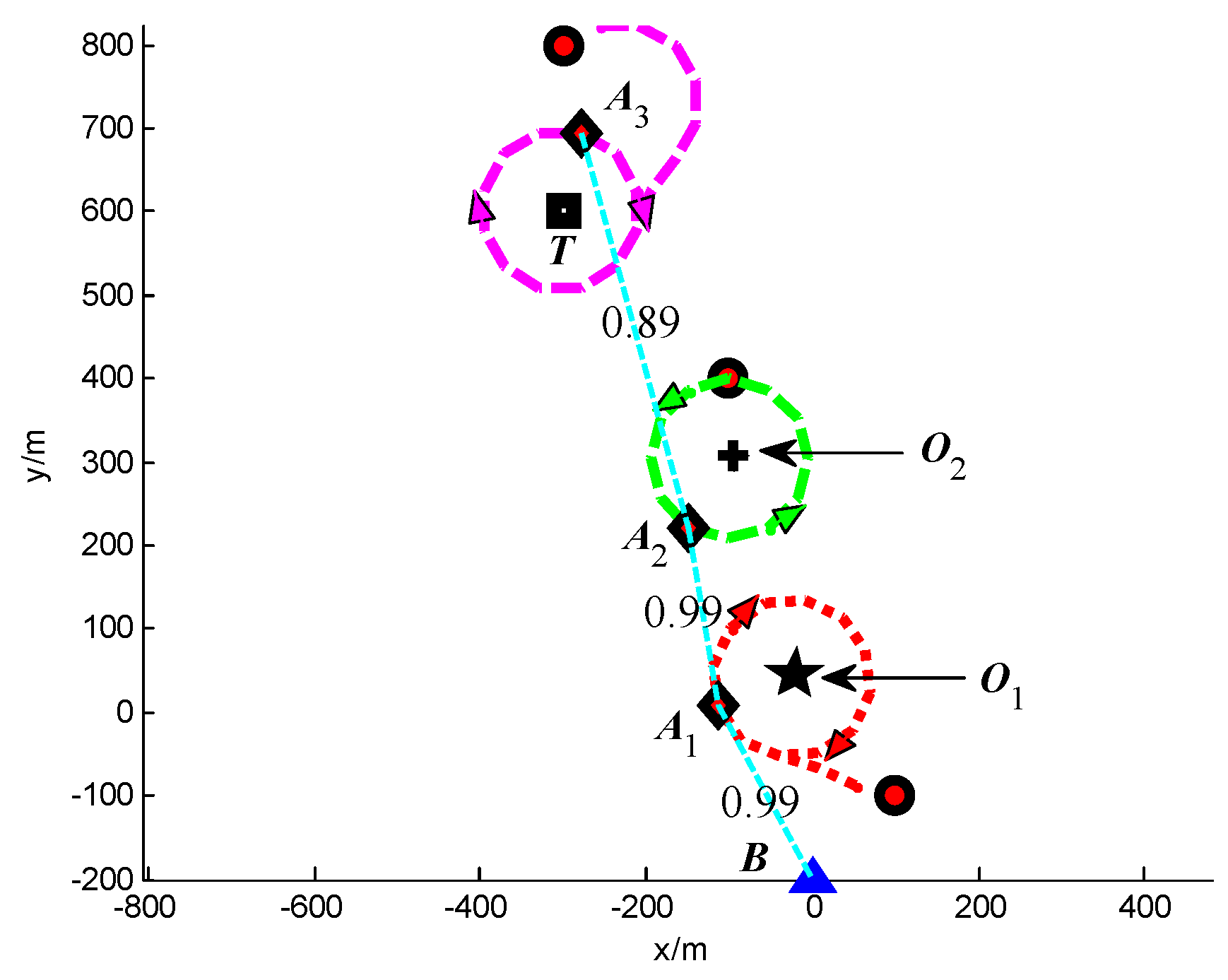
Figure 34.
Trajectories of UAVs at t = 100 s (Scenario 4).
Figure 34.
Trajectories of UAVs at t = 100 s (Scenario 4).
Figure 35.
The communication performances of A1, A2 and A3 (Scenario 4).
Figure 35.
The communication performances of A1, A2 and A3 (Scenario 4).
Figure 36.
The trace of FIM of A1, A2, A3 and base station (Scenario 4).
Figure 36.
The trace of FIM of A1, A2, A3 and base station (Scenario 4).
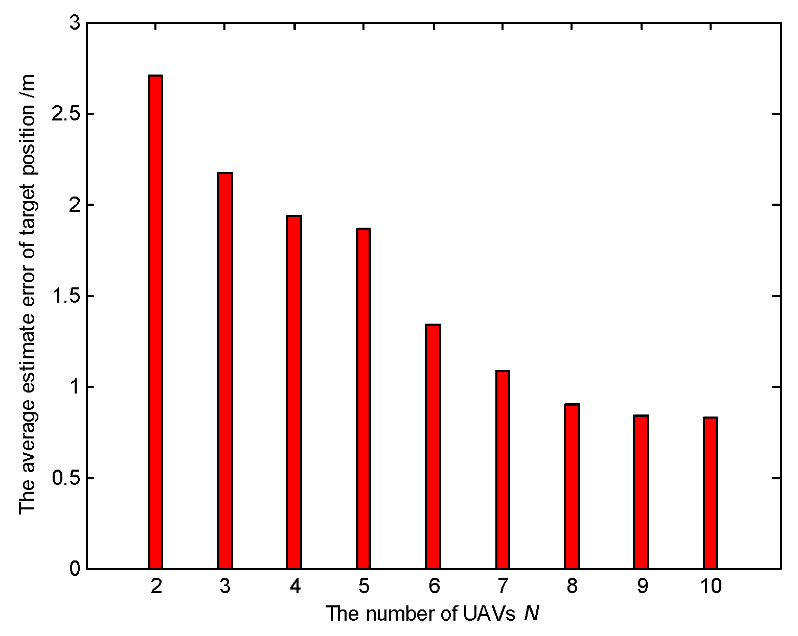
Figure 37.
The average estimation error of target position for different numbers of UAVs (Scenario 5).
Figure 37.
The average estimation error of target position for different numbers of UAVs (Scenario 5).
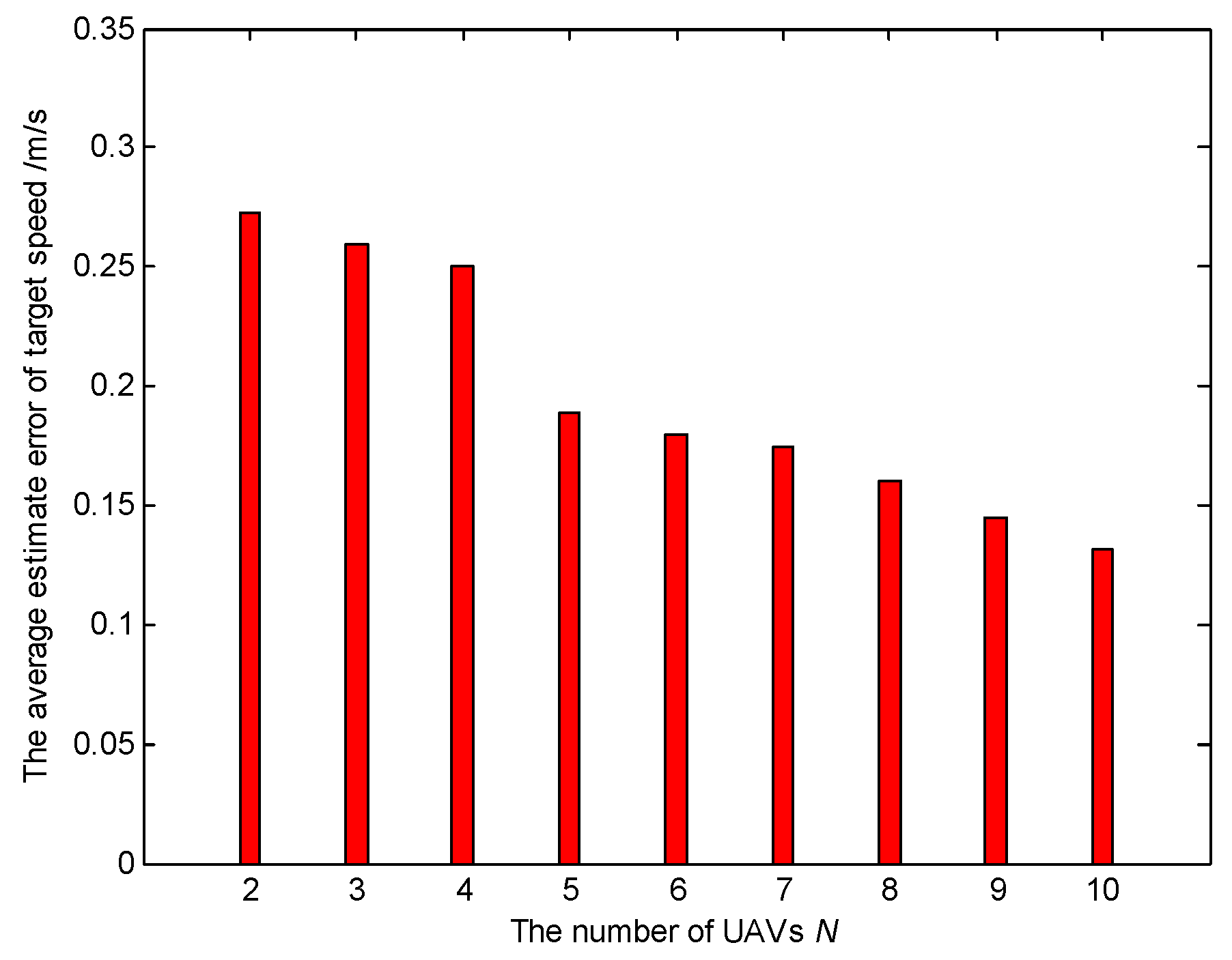
Figure 38.
The average estimation error of target speed for different numbers of UAVs (Scenario 5).
Figure 38.
The average estimation error of target speed for different numbers of UAVs (Scenario 5).
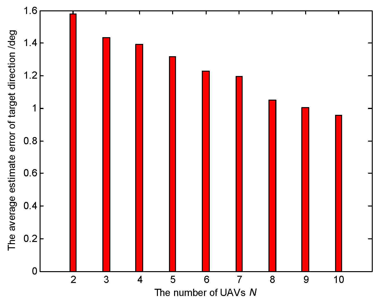
Figure 39.
The average estimation error of target direction for different numbers of UAVs (Scenario 5).
Figure 39.
The average estimation error of target direction for different numbers of UAVs (Scenario 5).
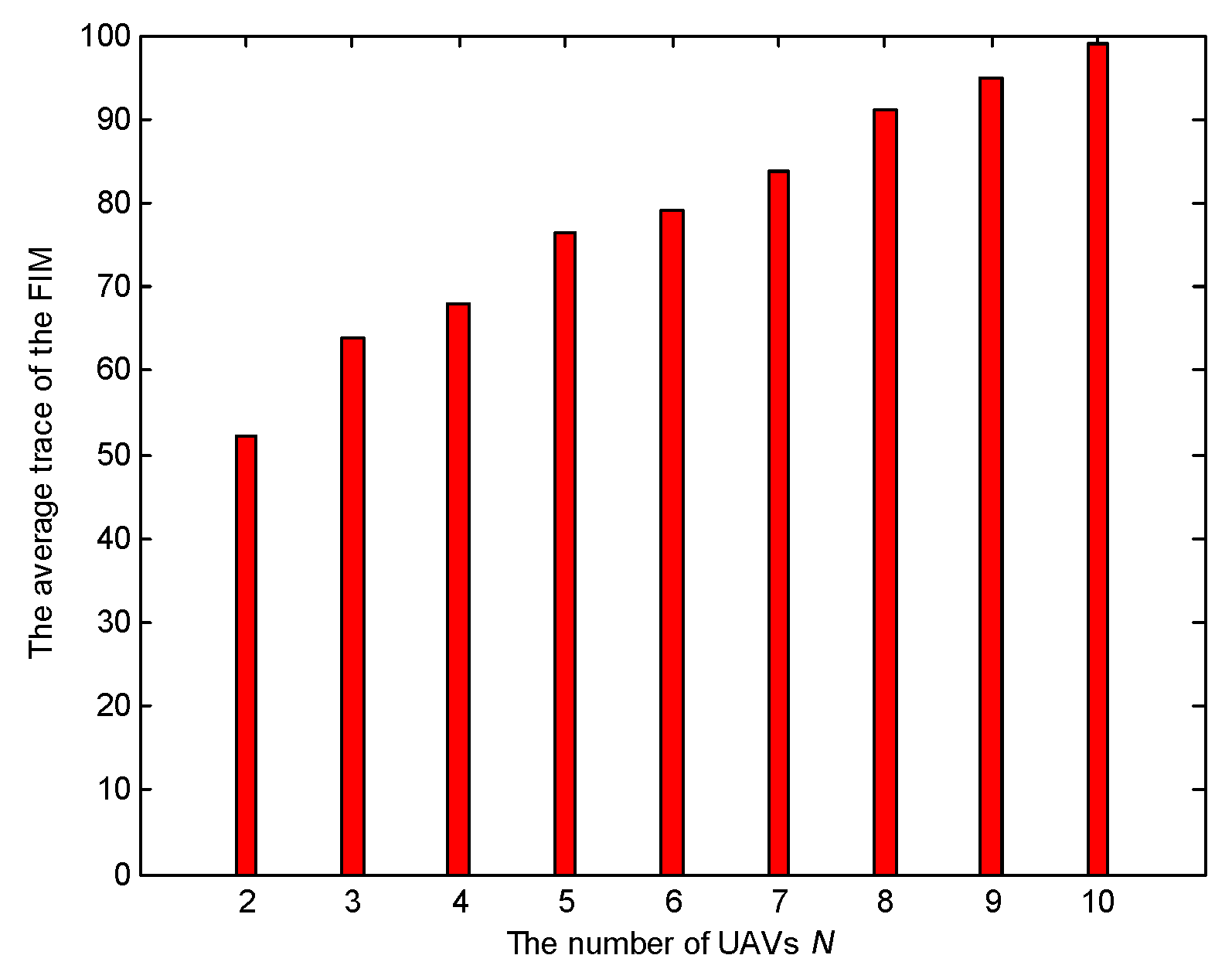
Figure 40.
The average trace of the FIM for different numbers of UAVs (Scenario 5).
Figure 40.
The average trace of the FIM for different numbers of UAVs (Scenario 5).
Table 1.
The parameters of the realistic wireless communication model.
Table 1.
The parameters of the realistic wireless communication model.
| Parameter | Value | Unit |
|---|
| Transmission power Pi | 30 | dBm |
| Noise power Nj | −70 | dBm |
| SNR requirement γ | 10 | - |
| Antenna gain constant Cij | 1 | - |
| Propagation loss factor α | 3 | - |
Table 2.
The initial settings of two UAVs in Scenario 1.
Table 2.
The initial settings of two UAVs in Scenario 1.
| UAV Ai | Position (xi, yi)/(m) | Heading Angle Ψi/(°) |
|---|
| A1 | (−400, −700) | 45 |
| A2 | (−800, 200) | 0 |
Table 3.
Comparison of the average estimate errors, the average transmission probabilities, and the average trace of the FIM in Scenario 1 (Group A vs. Group B).
Table 3.
Comparison of the average estimate errors, the average transmission probabilities, and the average trace of the FIM in Scenario 1 (Group A vs. Group B).
| Item | Group | Base Station | A1 | A2 |
|---|
| Average estimation error for position (m) | A | 1.2778 | 3.4806 | 1.9570 |
| B | 1.6287 | 2.4619 | 1.9565 |
| Average estimation error for speed (m/s) | A | 0.2100 | 0.3110 | 0.2714 |
| B | 0.2451 | 0.2931 | 0.2493 |
| Average estimation error for direction (°) | A | 1.2098 | 1.5951 | 1.3775 |
| B | 1.2133 | 1.5253 | 1.3121 |
| Average transmission probability | A | - | 0.8858 | 0.8056 |
| B | - | 0.7359 | 0.6203 |
| Average trace of the FIM | A | 72.4468 | 50.5545 | 55.9077 |
| B | 46.2311 | 52.0081 | 60.4408 |
Table 4.
The initial settings of the two UAVs in Scenario 2.
Table 4.
The initial settings of the two UAVs in Scenario 2.
| UAV Ai | Position (xi, yi)/(m) | Heading Angle Ψi/(°) |
|---|
| A1 | (−800, 200) | 45 |
| A2 | (−400, −700) | 180 |
Table 5.
Comparison of the average estimate errors, the average transmission probabilities, and the average trace of the FIM in Scenario 2 (Group A vs. Group B).
Table 5.
Comparison of the average estimate errors, the average transmission probabilities, and the average trace of the FIM in Scenario 2 (Group A vs. Group B).
| Item | Group | Base Station | A1 | A2 |
|---|
| Average estimation error for position (m) | A | 0.4266 | 0.7203 | 1.1680 |
| B | 0.5081 | 0.9029 | 0.7240 |
| Average transmission probability | A | - | 0.7463 | 0.9818 |
| B | - | 0.9209 | 0.6051 |
| Average trace of the FIM | A | 27.4777 | 14.6744 | 13.0033 |
| B | 15.5617 | 13.1899 | 14.2413 |
Table 6.
The initial settings of three UAVs in Scenario 3.
Table 6.
The initial settings of three UAVs in Scenario 3.
| UAV Ai | Position (xi, yi)/(m) | Heading Angle Ψi/(°) |
|---|
| A1 | (−400, −900) | 10 |
| A2 | (−800, 300) | 0 |
| A3 | (−800, 0) | 0 |
Table 7.
The average estimate errors, the average transmission probability, and the average trace of the FIM in Scenario 3.
Table 7.
The average estimate errors, the average transmission probability, and the average trace of the FIM in Scenario 3.
| Item | Base Station | A1 | A2 | A3 |
|---|
| Average estimation error for position (m) | 1.2454 | 6.2889 | 1.7638 | 4.0183 |
| Average estimation error for speed (m/s) | 0.2338 | 0.4282 | 0.2457 | 0.3552 |
| Average estimation error for direction (°) | 1.1365 | 1.1575 | 1.7017 | 1.4710 |
| Average transmission probability | - | 0.8485 | 0.4653 | 0.6953 |
| Average trace of the FIM | 72.4623 | 41.2674 | 57.2770 | 43.1731 |
Table 8.
The initial settings of three UAVs in Scenario 4.
Table 8.
The initial settings of three UAVs in Scenario 4.
| UAV Ai | Position (xi, yi)/(m) | Heading Angle Ψi/(°) |
|---|
| A1 | (100, −100) | 180 |
| A2 | (−100, 400) | 180 |
| A3 | (−300, 800) | 45 |
Table 9.
The average estimate errors, the average transmission probability, and the average trace of the FIM in Scenario 4.
Table 9.
The average estimate errors, the average transmission probability, and the average trace of the FIM in Scenario 4.
| Item | Base Station | A1 | A2 | A3 |
|---|
| Average estimation error for position (m) | 0.4535 | 1.2332 | 0.8105 | 0.4610 |
| Average transmission probability | - | 0.9818 | 0.9460 | 0.8894 |
| Average trace of the FIM | 40.7112 | 13.0033 | 13.1245 | 14.9834 |


