MPC and PSO Based Control Methodology for Path Tracking of 4WS4WD Vehicles

Abstract

Four wheel steering and four wheel drive (4WS4WD) vehicles are over-actuated systems with superior performance. Considering the control problem caused by the system nonlinearity and over-actuated characteristics of the 4WS4WD vehicle, this paper presents two methods to enable a 4WS4WD vehicle to accurately follow a predefined path as well as its reference trajectories including velocity and acceleration profiles. The methodologies are based on model predictive control (MPC) and particle swarm optimization (PSO), respectively. The MPC method generates the virtual inputs in the upper controller and then allocates the actual inputs in the lower controller using sequential quadratic programming (SQP), whereas the PSO method is proposed as a fully optimization based method for comparison. Both methods achieve optimization of the steering angles and wheel forces for each of four independent wheels simultaneously in real time. Simulation results achieved by two different controllers in following the reference path with varying disturbances are presented. Discussion about two methodologies is provided based on their theoretical analysis and simulation results.

1. Introduction

With the development of Autonomous Ground Vehicles (AGVs) in the last few decades, the demand for accuracy, maneuverability and controllability in vehicle’s navigation is ever increasing. For example, an AGV may be required to follow a path accurately under unstructured and uneven terrain conditions, where a significant amount of wheel slip and unpredictable disturbance forces occur at the vehicle’s wheels. The 4WS4WD vehicle, with four wheels that can be steered and driven independently, is a revolutionary platform that has great potential to perform high maneuverability and flexibility in harsh environments.

The main challenge in the control of 4WS4WD control is the number of control inputs (four steering angles and four drive torques), which results in an over-actuated system, where only three outputs including its degree of freedom (DOF) in the longitudinal, lateral and angular directions of the vehicle are concerned. How to allocate all eight control inputs to achieve high path following performance has not yet been effectively solved. The control allocation is proposed to handle the control problems of over-actuated systems [1]. Generally, the control allocation can be treated as an optimization problem.

For controller designing, a model of the vehicle under control is generally required to facilitate the selection of future control inputs. A dynamic model describes the states of the vehicle based on the forces applied. However, the development of a detailed vehicle dynamic model is always a challenging task due to the uncertainty of parameters and the complex disturbances from the external forces. The majority of existing control methodologies for 4WS4WD vehicles are proposed based on the linearized dynamic model, which lead to the loss of input degree of freedom [2,3]. Meanwhile, some other methods use nonlinear dynamic models in the control of 4WS4WD vehicles [4,5], where control inputs are subjected to some relationship constraints to simplify the controller design. However, in practice, the four independent wheels may interact with different terrain conditions, where different slip, wheel forces and terrain disturbances are generated on the corresponding contact patches. Hence, it is desirable to make four wheels individually controlled, thereby limiting and/or overcoming different slip and disturbance on different contact patch.

There is an abundance of literature that presents kinematic modelling of ground vehicles [6,7,8], in which the vehicles are assumed to operate at low speeds to reduce the dynamic effects. Most vehicle kinematic models are developed based on the non-integrable kinematic constraints, known as non-holonomic constraints. As a result, the wheel slip has to be ignored with the assumption of zero relative velocity between wheels and terrain [9,10]. To utilize the kinematic model’s advantage of keeping the steering control relatively independent of velocity control [11], it is desirable to incorporate wheel slip in the vehicle kinematic model so as to facilitate the accurate vehicle control in complex terrain conditions where the no-slip assumption is not applicable.

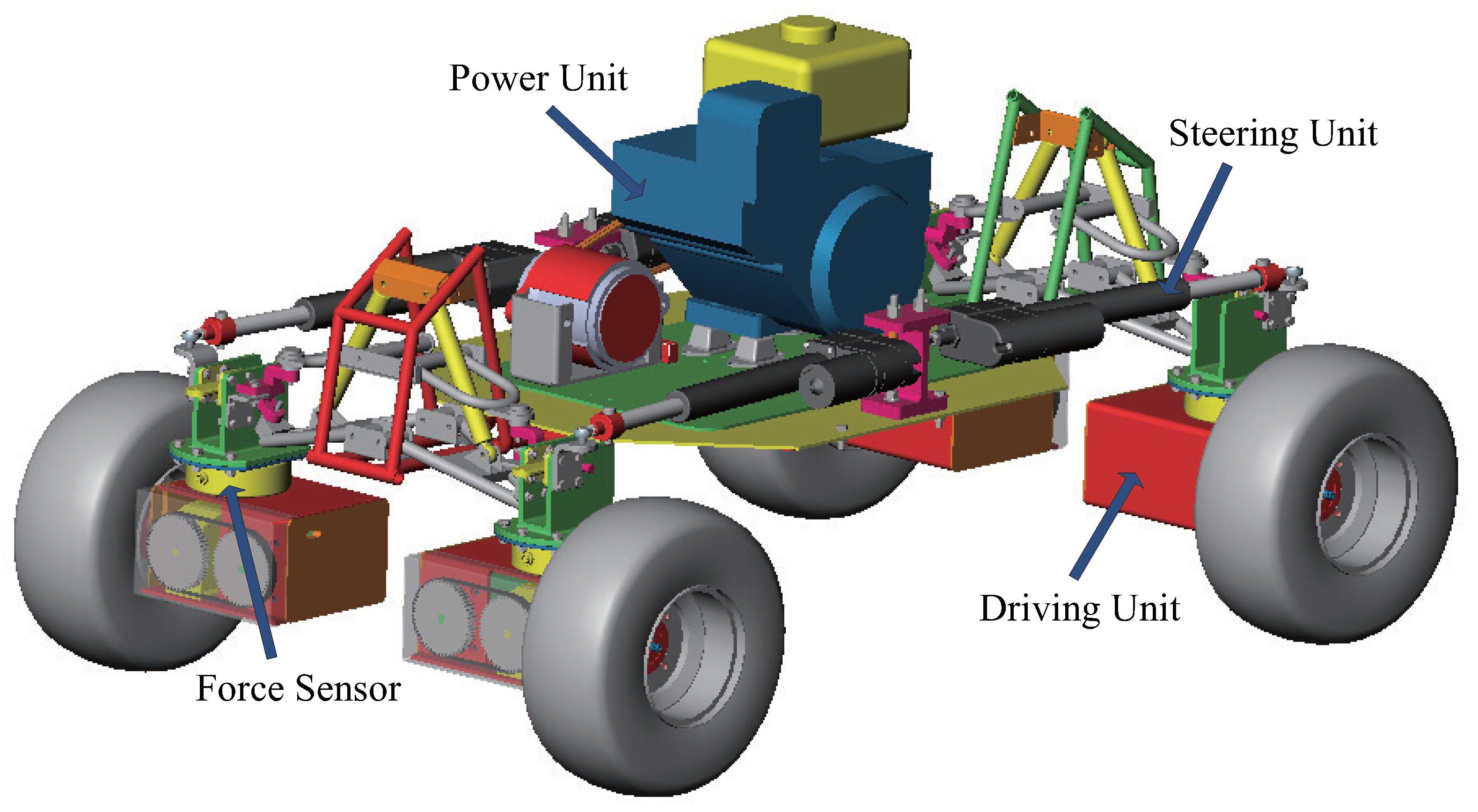
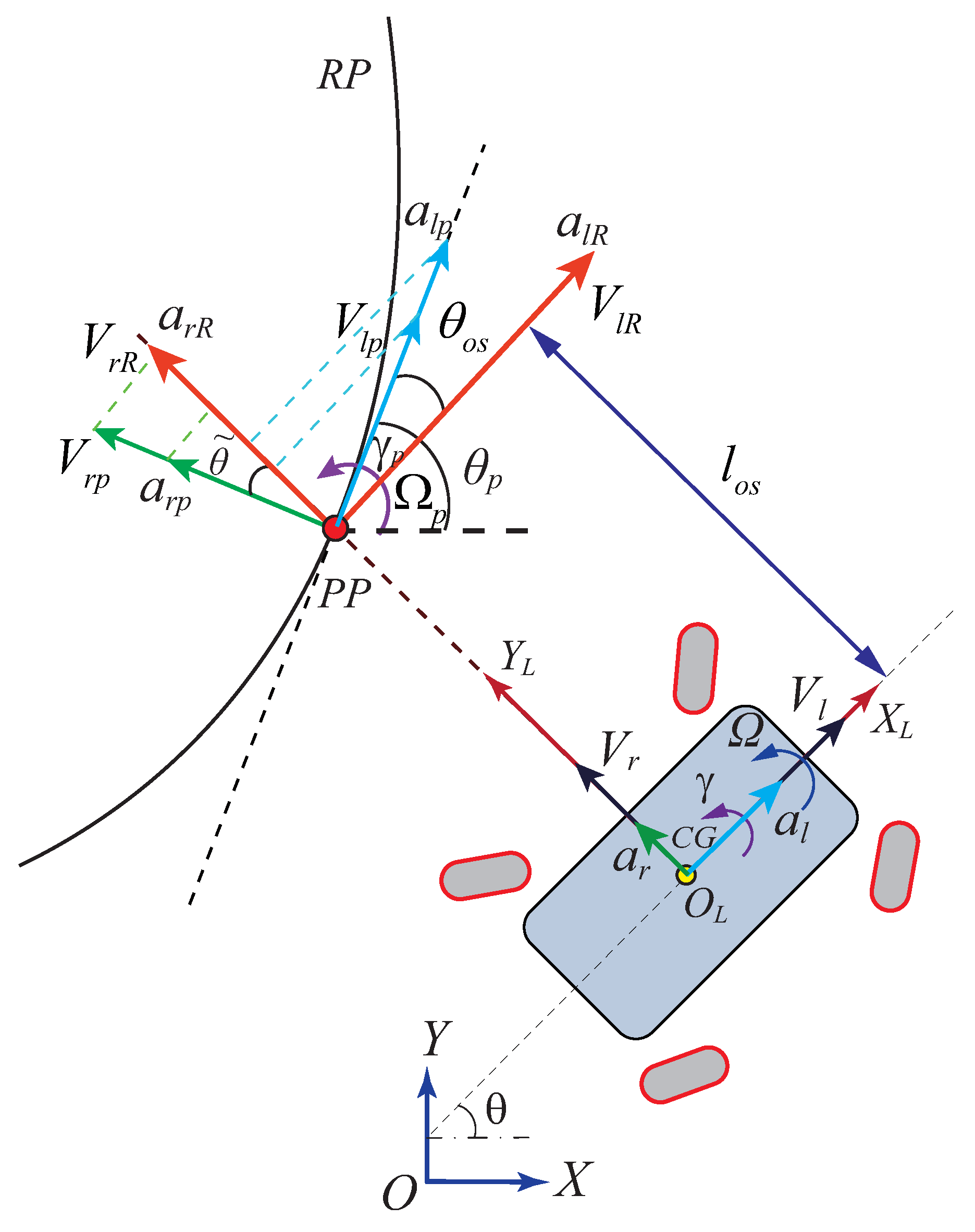
To realize force control, a novel type of 4WS4WD vehicle with force sensors at each wheel has been designed as shown in Figure 1. This vehicle possesses the characteristics of independent steering and drive control at each wheel and force measurements. In this work, the dynamic model is partitioned into a hierarchy of three levels to facilitate the incorporation of force sensors and overcome uncertainties in the model. The force sensors at the drive unit allow the measurement of actual force data, while models of the drive unit and tire are used for simulation.

Model predictive control (MPC) is selected for its ability in handling linear constraints and time-varying systems as well as its good performance in tracking problems. Particle swarm optimization (PSO) is also selected for its fast searching speed in global optimization. MPC and PSO have been successfully applied in the controller design of real-time control systems [12,13,14,15,16,17]. In this work, MPC and PSO based control methods are proposed to realize the controlling aim of achieving good path following performance as well as high motion quality via vehicle steering control and independent force control at four wheels.

As novel contributions, the MPC methodology is applied to achieve precise path tracking of 4WS4WD vehicle. Based on the MPC theory, an offline control law is proposed to guarantee the stability of the upper controller. An sequential quadratic programming (SQP) based control allocation is developed to control the 4WS4WD vehicle in the lower controller. The inclusion of full independent force control and steering control on all four wheels enable the maximization of performance. In this work, comparison of MPC and PSO on the same vehicle model is provided, in which the proposed PSO control methodology is a further refinement of the PSO methodology presented previously in [18]. The PSO control methodology in this paper simplifies the derivation and gives an algorithm in a more general form, which facilitates the comparison with other control methods. In addition, both methodologies are compared with the kinematic model based method proposed in [19].

The paper is organized as follows: Section 2 describes the 4WS4WD vehicle modelling. The MPC and PSO control methodologies are presented in Section 3. In Section 4, simulation setup and the reference path are presented. The result of the two controllers are compared. In Section 5, the discussion about two methodologies are provided based on their theoretical analysis and simulation results. Finally, conclusions are provided in Section 6.

2. Vehicle System Modelling

In order to develop suitable control methodology, the 4WS4WD vehicle must be modelled for controller design and simulation. The model used for this work is a fully dynamic model that consists of three components, vehicle body dynamics to estimate vehicle body movement, drive unit dynamics to model the tire force acting on the drive unit in vehicle coordinate frame and a tire dynamic model to model the force generated by the tire in a wheel coordinate frame. The separation of dynamic model allows force sensors to be incorporated easily and reduces uncertainties by obtaining actual force measurements. In the end, an offset error model is proposed for evaluating the tracking performance and is used in the controller design.

2.1. Vehicle Body Dynamic Model

As shown in Figure 2, the vehicle body dynamic model describes the motion of the vehicle by representing each drive unit as a pair of forces, with $F_{Sl}$ in the longitudinal and $F_{SL}$ in the lateral direction of the corresponding wheel. The reason for separating the dynamics of the vehicle at the drive unit boundary is to allow force sensors to be incorporated to measure the forces acting on each wheel, instead of relying on the tire model to estimate them. To facilitate the notations, the four wheels are numbered by 1, 2, 3 and 4 in circles. In particular, the force acting at each force sensor is decomposed into two components (i.e., $F_{Sli}$ and $F_{SLi}$, $i=1,\dots ,4$) normal to each other.

The equation of the vehicle body dynamics can be expressed as

$$\mathit{acc}=\left[\begin{array}{c}{a}_r\\ a_l\\ \gamma \end{array}\right]={\mathit{M}}^{-1}\mathit{C}\left[\begin{array}{c}{R}_1{\mathit{F}}_{AS1}\\ R_2{\mathit{F}}_{AS2}\\ R_3{\mathit{F}}_{AS3}\\ R_4{\mathit{F}}_{AS4}\end{array}\right],$$

(1)

where the acceleration vector denoted by $\mathit{acc}$ consists of longitudinal acceleration $a_l$, radial acceleration $a_r$ and angular acceleration $\gamma$.

The mass matrix is represented by $\mathit{M}$:

$$\mathit{M}=\left[\begin{array}{ccc}M-4m_d& 0& 0\\ 0& M-4m_d& 0\\ 0& 0& J_z\end{array}\right],$$

(2)

where M is the mass of the vehicle, $J_z$ is the vehicle body inertia, and $m_d$ is the mass of the drive unit.

The matrix $\mathit{C}$ is decided by vehicle dimension, written as

$$\mathit{C}=\left[\begin{array}{cccccccc}1& 0& 1& 0& 1& 0& 1& 0\\ 0& 1& 0& 1& 0& 1& 0& 1\\ -L_h& L_f& L_h& L_f& L_h& -L_r& -L_h& -L_r\end{array}\right].$$

(3)

The force vectors ${\mathit{F}}_{ASi}$ are defined as

$${\mathit{F}}_{ASi}={\left[\begin{array}{cc}{F}_{Sli}& F_{SLi}\end{array}\right]}^T,i=1,\dots ,4.$$

(4)

The transfer matrices $R_i$ from wheel frame to vehicle local coordinate frame $X_L-O_L-Y_L$ are presented in

$$R_i=\left[\begin{array}{cc}cos{\delta }_i& -sin{\delta }_i\\ sin{\delta }_i& cos{\delta }_i\end{array}\right],i=1,\dots ,4.$$

(5)

The lateral components $F_{SLi}$ are determined by the lateral forces acting on tires, while the longitudinal components $F_{Sli}$ are viewed as intermediate control inputs of vehicle system, which can be achieved by controlling the torques (i.e., $T_i$, $i=1,\dots ,4$) applied on wheels. To simplify the coupled issue of left and right wheel steerings, the steering angles are constrained by

$$\begin{array}{c}\hfill {\delta }_1={\delta }_2={\delta }_f,\\ \hfill {\delta }_3={\delta }_4={\delta }_r.\end{array}$$

(6)

Therefore, the vehicle system in this work considers six control inputs (i.e., ${\delta }_f$, ${\delta }_r$ and $T_i$, $i=1,\dots ,4$) in total.

2.2. Driving Unit Dynamic Model

While the force sensors provide measurement of the current forces acting on each wheel, controller design requires prediction of future values based on control inputs. The drive unit dynamic model as shown in Figure 3 is described in this section.

In each driving unit, the force sensor mounted on the wheel hub rotate with the wheel. Force measurement is in the direction of the steering angle. According to Figure 3, the dynamics of driving unit can be expressed by

$${\mathit{F}}_{ASi}={\left[\begin{array}{cc}{F}_{Sli}& F_{SLi}\end{array}\right]}^T={\mathit{F}}_{wi}-{\left[\begin{array}{cc}{m}_d{a}_{wli}& m_d{a}_{wLi}\end{array}\right]}^T,$$

(7)

where $a_{wli}$ and $a_{wLi}$ denote the longitudinal and lateral accelerations of each driving unit i in the wheel coordinate system ($X_{Wi}-O_{Wi}-Y_{Wi}$), respectively. Using the transfer matrices $R_i$ and the accelerations $a_l$, $a_r$ and $\gamma$ given in vehicle body dynamic model, $a_{wli}$ and $a_{wLi}$ can be deduced as

$$\begin{array}{c}\hfill \left[\begin{array}{cc}{a}_{wl1}& a_{wL1}\end{array}\right]=\left[\begin{array}{cc}{a}_l-L_h\gamma & a_r+L_f\gamma \end{array}\right]R_1,\\ \hfill \left[\begin{array}{cc}{a}_{wl2}& a_{wL2}\end{array}\right]=\left[\begin{array}{cc}{a}_l+L_h\gamma & a_r+L_f\gamma \end{array}\right]R_2,\\ \hfill \left[\begin{array}{cc}{a}_{wl3}& a_{wL3}\end{array}\right]=\left[\begin{array}{cc}{a}_l+L_h\gamma & a_r-L_r\gamma \end{array}\right]R_3,\\ \hfill \left[\begin{array}{cc}{a}_{wl4}& a_{wL4}\end{array}\right]=\left[\begin{array}{cc}{a}_l-L_h\gamma & a_r-L_r\gamma \end{array}\right]R_4.\end{array}$$

(8)

In Equation (7), ${\mathit{F}}_{wi}$ represents the force vector acting on each wheel, which is written as

$${\mathit{F}}_{wi}={\left[\begin{array}{cc}{F}_{wli}& F_{wLi}\end{array}\right]}^T.$$

(9)

2.3. Tire Model

The actual generation of wheel forces are from the contact between tires and the ground. The wheel forces depend on the surface friction, load, and the intrinsic properties of the tire. To analyze the wheel forces ${\mathit{F}}_{wi}$ in Equation (9), the tire model is built as shown in Figure 4.

Considering the generation of wheel forces and external disturbances, ${\mathit{F}}_{wi}$ can be expressed as

$${\mathit{F}}_{wi}={\left[\begin{array}{cc}{F}_{wli}& F_{wLi}\end{array}\right]}^T={\left[\begin{array}{cc}{F}_{li}-F_{gli}& F_{Li}-F_{gLi}\end{array}\right]}^T,$$

(10)

where $F_{li}$ and $F_{Li}$ ($i=1,\dots ,4$) are longitudinal and lateral forces caused by wheel slip, respectively. $F_{gli}$ and $F_{gLi}$ denote the terrain disturbances corresponding to $F_{li}$ and $F_{Li}$.

According to [20], the longitudinal force can be considered proportional to the slip ratio in small range, which is expressed by

$$F_{li}=\left\{\begin{array}{c}{k}_{li}{F}_{Ni}\frac{{\varsigma }_i}{0.1},\left|{\varsigma }_i\right|\le 0.1,\\ k_{li}{F}_{Ni},\left|{\varsigma }_i\right|>0.1,\end{array}\right.$$

(11)

where $F_{Ni}$ is the weight force on wheel i. In the simulation, the load transfer due to the longitudinal and lateral accelerations and roll angle are taken into consideration. $F_{Ni}$ can be calculated by considering longitudinal and lateral load transfer according to [21]. The longitudinal slip stiffness $k_{li}$ is determined by the tire type and terrain condition. ${\varsigma }_i$ is the longitudinal slip ratio of wheel i presented in [22]:

$${\varsigma }_i=\left\{\begin{array}{l}{\displaystyle \frac{R_w{\omega }_i-v_{wi}}{R_w{\omega }_i}},R_w{\omega }_i>v_{wi}>0,\\ {\displaystyle \frac{R_w{\omega }_i-v_{wi}}{v_{wi}}},R_w{v}_{wi}>{\omega }_i>0,\\ 0,R_w{v}_{wi}={\omega }_i\ge 0,\end{array}\right.$$

(12)

where $R_w$ and ${\omega }_i$ denote the tire radius and angular velocity of wheel i as shown in Figure 4b. $v_{wi}$ represents the actual velocity of the wheel i, which can be calculated by the vehicle geometry as well as velocities $V_l$, $V_r$ and $\Omega$ shown in Figure 2. Note that the model is proposed only considering the vehicle is moving forward. Thus, $v_{wi}$ and ${\omega }_i$ are set to be nonnegative. As is discussed in Equation (12), the slip ratio is zero when the vehicle is resting.

Finally, as per Figure 4b, the wheel dynamic equation indicating the relationship between $T_i$ and $F_{li}$ can be written as

$$T_i=(F_{li}+F_{ri})R_w+{\dot{\omega }}_i{J}_w,$$

(13)

where $J_w$ represents the wheel inertia, and $F_{ri}$ is the rolling resistance calculated by

$$F_{ri}=F_{Ni}(K_{r0}+K_{r1}{V}_l^2),$$

(14)

where $K_{r0}=0.015$ and $K_{r1}=7\times {10}^{-6}$ s${}^2$/m${}^2$ are the parameters for common car tires [23].

The steering motion of wheels result in the lateral slip velocities $v_{si}$, which causes the actual direction of wheel velocity $v_{wi}$ to differ from the wheel center plane by the slip angle ${\alpha }_i$. According to the tire lateral characteristic curve [24], a linear model for $F_{Li}$ is given in

$$F_{Li}=\left\{\begin{array}{c}-k_{Li}{F}_{Ni}\frac{{\alpha }_i}{5},\left|{\alpha }_i\right|\le 5^{°},\\ -k_{Li}{F}_{Ni},{\alpha }_i>5^{°},\\ k_{Li}{F}_{Ni},{\alpha }_i<-5^{°},\end{array}\right.$$

(15)

where $k_{Li}$ is the lateral slip stiffness of the wheel i. Note that, due to the sign conventions in $X_{Wi}-O_{Wi}-Y_{Wi}$ and $X_L-O_L-Y_L$, a negative slip angle causes a positive lateral force and vice versa.

As shown in Figure 4a, the slip angle ${\alpha }_i$ can be calculated by steering angle ${\delta }_i$ and side slip angle ${\beta }_i$,

$${\alpha }_i={\beta }_i-{\delta }_i,$$

(16)

where the expression of ${\beta }_i$ is available in our previous work presented in [25].

2.4. Offset Model

An offset error model is proposed for the evaluation of the performance of the controllers. The reference position (RP) of the vehicle on the reference path is defined as the normal projection of the heading of the vehicle at the centre of gravity on to the reference path, as shown in Figure 5. The tracking error in vehicle coordinate frame consists of lateral offset error $l_{os}$ and heading error ${\theta }_{os}$, expressed as

$$\widetilde{\mathit{pos}}={\left[\begin{array}{ccc}0& l_{os}& {\theta }_{os}\end{array}\right]}^T$$

(17)

The position errors are always in the lateral direction of the vehicle. The longitudinal position error is set to 0. The heading error can be found by

$${\theta }_{os}=\theta -{\theta }_{ref},$$

(18)

where ${\theta }_{ref}$ is the reference heading direction of the RP, tangential to the reference path.

The velocity error states $\widetilde{\mathit{vel}}$ is the difference between vehicle velocity $\mathit{vel}$ and reference velocity states ${\mathit{vel}}_{ref}$ in the vehicle coordinate frame. $\widetilde{\mathit{vel}}$ can be expressed as

$$\widetilde{\mathit{vel}}={\left[\begin{array}{ccc}{V}_{lerr}& V_{rerr}& {\Omega }_{err}\end{array}\right]}^T=\mathit{vel}-{\mathit{vel}}_{ref},$$

(19)

where $V_{lerr}$, $V_{rerr}$ and ${\Omega }_{err}$ are the errors in longitudinal, lateral, and angular velocity, respectively. Reference velocity states are defined as

$${\mathit{vel}}_{ref}={\left[\begin{array}{ccc}{V}_{lref}& V_{rref}& {\Omega }_{ref}\end{array}\right]}^T,$$

(20)

where reference angular velocity ${\Omega }_{ref}$ is the rate of change of the heading of RP on the reference path.

The reference longitudinal velocity $V_{lref}$ and lateral velocity $V_{rref}$ in vehicle coordinate frames can be derived from the reference path coordinate frame by the equations:

$$\begin{array}{c}\hfill V_{lref}=V_{lp}cos\left({\theta }_{os}\right)-V_{rp}sin\left({\theta }_{os}\right),\\ \hfill V_{rref}=V_{lp}sin\left({\theta }_{os}\right)+V_{rp}cos\left({\theta }_{os}\right),\end{array}$$

(21)

where $V_{lp}$ is the reference longitudinal velocity, taken as tangential to the reference path. $V_{rp}$ is the reference radial velocity normal to the reference path at RP.

Finally, the acceleration error states $\widetilde{\mathit{acc}}$ are written as:

$$\widetilde{\mathit{acc}}={\left[\begin{array}{ccc}{a}_{lerr}& a_{rerr}& {\gamma }_{err}\end{array}\right]}^T=\mathit{acc}-{\mathit{acc}}_{ref},$$

(22)

where $\mathit{acc}$ is the difference between vehicle acceleration $\mathit{acc}$ and reference acceleration ${\mathit{acc}}_{ref}$. The reference acceleration vector ${\mathit{acc}}_{ref}$ is defined as

$${\mathit{acc}}_{ref}={\left[\begin{array}{ccc}{a}_{lref}& a_{rref}& {\gamma }_{ref}\end{array}\right]}^T,$$

(23)

where $a_{lref}$ and $a_{rref}$ are, respectively, the reference longitudinal and lateral acceleration at point RP, measured in the direction and normal to the vehicle heading, and ${\gamma }_{ref}$ is the reference angular acceleration of the point RP.

The reference acceleration in vehicle coordinate frame can be derived from the path coordinate frame by

$$\begin{array}{c}\hfill a_{lref}=a_{lp}cos\left({\theta }_{os}\right)-a_{rp}sin\left({\theta }_{os}\right),\\ \hfill a_{rref}=a_{lp}sin\left({\theta }_{os}\right)+a_{rp}cos\left({\theta }_{os}\right),\end{array}$$

(24)

where $a_{lp}$ and $a_{rp}$ are the reference acceleration tangential and normal to the reference path.

3. Control Methodology

Two methods of finding the optimal control inputs for steering angles (i.e., ${\delta }_f$ and ${\delta }_r$) and drive forces $F_{Sli},(i=1,\dots ,4)$ are developed. The first method used model predictive control (MPC) with a sequential quadratic programming (SQP) solver. The second method is particle swarm optimization (PSO). The objective of the controller is to accurately follow a predetermined path through multiple terrain types.

3.1. MPC-SQP Method

3.1.1. Offset Model Linearization

In order to be applied in the MPC controller design, the offset model is linearized by a feedback linearization method. By defining the state vector $\mathit{x}=[x_1,x_2,x_3,x_4,x_5]$, as $x_1=V_{lerr}$, $x_2=l_{os}$, $x_3={\dot{l}}_{os}$, $x_4={\theta }_{os}$ and $x_5={\dot{\theta }}_{os}$, the offset model can be written in the following form:

$$\begin{array}{cc}\hfill {\dot{x}}_1=& a_r-(a_{lp}cos{x}_4-a_{rp}sin{x}_4),\hfill \\ \hfill {\dot{x}}_2=& x_3,\hfill \\ \hfill {\dot{x}}_3=& a_r-(a_{lp}sin{x}_4+a_{rp}cos{x}_4),\hfill \\ \hfill {\dot{x}}_4=& x_5,\hfill \\ \hfill {\dot{x}}_5=& \gamma -{\gamma }_{ref}.\hfill \end{array}$$

(25)

In this model, $a_r$, $a_l$ and $\gamma$ are considered as the inputs while other constants including reference accelerations and velocities can be obtained from the vehicle states. The nonlinearity of the model comes from trigonometric terms of $x_4$. For accurate path tracking problems, the yaw error is assumed to vary smoothly within [−10° 10°]. Then, the model can be linearized by feedback linearization. Define the input vector $\mathit{u}={\left[a_r{a}_l\gamma \right]}^T$; then, the new input vector at time $t_k$ is obtained as

$${\mathit{v}(\mathit{x},t)|}_{t=t_k}=\mathit{u}-{\left[\begin{array}{c}{a}_{lp}cos{x}_4-a_{rp}sin{x}_4\\ a_{lp}sin{x}_4+a_{rp}cos{x}_4\\ {\gamma }_{ref}\end{array}\right]}_{x_4=x_4\left(t_k\right)},$$

(26)

and the offset model is expressed as

$$\dot{\mathit{x}}{=\mathit{A}·\mathit{x}+\mathit{v}(\mathit{x},t)|}_{t=t_k},$$

(27)

where

$$\begin{array}{c}\hfill \mathit{A}=\left[\begin{array}{ccccc}0& 0& 0& 0& 0\\ 0& 0& 1& 0& 0\\ 0& 0& 0& 0& 0\\ 0& 0& 0& 0& 1\\ 0& 0& 0& 0& 0\end{array}\right].\end{array}$$

It can be seen that the model is time-varying but can be treated as a linear model at each sampling step. The output vector is denoted by ${\mathit{y}}_c$ and the equation is written as

$${\mathit{y}}_c={\mathit{C}}_c\mathit{x},$$

(28)

where

$$\begin{array}{cc}\hfill {\mathit{C}}_c=& \left[\begin{array}{ccc}1& 0& 0\\ 0& 1& 0\\ 0& 0& 0\\ 0& 0& 1\\ 0& 0& 0\end{array}\right].\hfill \end{array}$$

3.1.2. Model Predictive Control

To develop the MPC controller, the offset model as given in Equations (27) and (28) needs to be discretized and its discrete-time state vector form can be written as

$$\begin{array}{cc}\hfill {\mathit{x}}_d(k+1)=& {\mathit{A}}_d{\mathit{x}}_d\left(k\right)+{\mathit{B}}_d{\mathit{u}}_d\left(k\right),\hfill \\ \hfill {\mathit{y}}_d\left(k\right)=& {\mathit{C}}_d{\mathit{x}}_d\left(k\right),\hfill \end{array}$$

(29)

where ${\mathit{x}}_d\left(k\right)$, ${\mathit{y}}_d\left(k\right)$ and ${\mathit{u}}_d\left(k\right)$ are the state vector, output vector and input vector, respectively. The coefficient matrices ${\mathit{A}}_d$, ${\mathit{B}}_d$ and ${\mathit{C}}_d$ are updated after discretization.

To eliminate undesirable oscillations, embedded integrator vectors $\Delta {\mathit{x}}_d\left(k\right)={\mathit{x}}_d(k+1)-{\mathit{x}}_d\left(k\right)$, $\Delta \mathit{u}\left(k\right)={\mathit{u}}_d(k+1)-{\mathit{u}}_d\left(k\right)$ are defined, thereby an augmented state-space model can be expressed as

$$\begin{array}{cc}\hfill \left[\begin{array}{c}\Delta {\mathit{x}}_d(k+1)\\ {\mathit{y}}_d(k+1)\end{array}\right]=& \left[\begin{array}{cc}{\mathit{A}}_d& {\mathit{O}}^T\\ {\mathit{C}}_d{\mathit{A}}_d& \mathit{I}\end{array}\right]\left[\begin{array}{c}\Delta {\mathit{x}}_d\left(k\right)\\ {\mathit{y}}_d\left(k\right)\end{array}\right]+\left[\begin{array}{c}{\mathit{B}}_d\\ {\mathit{C}}_d{\mathit{B}}_d\end{array}\right]\Delta \mathit{u}\left(k\right),\hfill \\ \hfill {\mathit{y}}_d\left(k\right)=& \left[\begin{array}{cc}\mathit{O}& \mathit{I}\end{array}\right]\left[\begin{array}{c}\Delta {\mathit{x}}_d\left(k\right)\\ {\mathit{y}}_d\left(k\right)\end{array}\right],\hfill \end{array}$$

(30)

where $\mathit{O}$ is a zero matrix, and $\mathit{I}$ represents the identity matrix.

Defining the new state vector $\mathit{x}\left(k\right)={[\Delta {\mathit{x}}_d{\left(k\right)}^T{\mathit{y}}_d{\left(k\right)}^T]}^T$, the augmented model can be written in the following matrix form:

$$\begin{array}{cc}\hfill \mathit{x}(k+1)=& \mathit{A}\mathit{x}\left(k\right)+\mathit{B}\Delta \mathit{u}\left(k\right),\hfill \\ \hfill \mathit{y}\left(k\right)=& \mathit{C}\mathit{x}\left(k\right),\hfill \end{array}$$

(31)

where

$$\begin{array}{cc}\hfill \mathit{A}& =\left[\begin{array}{cc}{\mathit{A}}_d& {\mathit{O}}^T\\ {\mathit{C}}_d{\mathit{A}}_d& \mathit{I}\end{array}\right],\mathit{B}=\left[\begin{array}{c}{\mathit{B}}_d\\ {\mathit{C}}_d{\mathit{B}}_d\end{array}\right],\mathit{C}=\left[\begin{array}{cc}{\mathit{O}}^T& \mathit{I}\end{array}\right].\hfill \end{array}$$

Theorem 1.

Given a discrete time system following the form of Equation (31), the asymptotic stabilization of the closed-loop system can be realized by substituting the first item of $\Delta {\mathit{U}}^{\ast }$ as the control input $\Delta u\left(k\right)$ , when $\Delta {\mathit{U}}^{\ast }$ is the optimal solution of the following optimization problem:

$$\begin{array}{c}arg\underset{\Delta \mathit{U}}{min}J={({\mathit{R}}_s-\mathit{Y})}^T({\mathit{R}}_s-\mathit{Y})+\Delta {\mathit{U}}^T\overline{R}\Delta \mathit{U},\hfill \\ s.t.y_{N_p}(\Delta \mathit{U})=0,\hfill \end{array}$$

(32)

where $\mathit{Y}$ denotes the predicted output sequence, $\Delta \mathit{U}$ denotes the future input sequence, and $N_p$ is the prediction horizon. $R_s$ is the sequence of the control target vector. $y_{N_p}(\Delta \mathit{U})$ represents the error between the final predicted output and target.

Proof of Theorem 1.

To prove the stability, the Lyapunov function $V\left(x_k\right)$ is defined equal to the value of the objective function $J_k$ subjected to its optimal solution, which can be expressed as

$$\begin{array}{cc}\hfill V\left(x_k\right)& =min{J}_k\hfill \\ & =\sum _{i=1}^{N_p}{y}_{k+i}^T{y}_{k+i}+\sum _{i=0}^{N_p-1}\Delta u_{k+i}^T{r}_w\Delta u_{k+i},\hfill \end{array}$$

(33)

where, $\Delta u_k,\dots ,\Delta u_{k+N_p-1}$ are obtained by the optimal solution of future inputs, and $y_k,\dots ,y_{k+N_p}$ represent the corresponding error sequence between future outputs and target. $r_w$ is the nonnegative gain matrix.

According to the definition in Equation (33), the Lyapunov function at the next sample $k+1$ is written as

$$\begin{array}{c}\hfill V\left(x_{k+1}\right)=\sum _{i=1}^{N_p}{y}_{k+1+i}^T{y}_{k+1+i}+\sum _{i=0}^{N_p-1}\Delta u_{k+1+i}^T{r}_w\Delta u_{k+1+i}.\end{array}$$

(34)

To facilitate the comparison between two neighboring Lyapunov function values, a intermediate function $\overline{V}$ is defined, which is formed by evaluating $V\left(x_{k+1}\right)$ with a defined inputs sequence, which is obtained by shifting the optimal inputs sequence of $V\left(x_{ki}\right)$ one step forward, and setting its last input $\Delta u_{k+N_p}$ as zero. It is obvious that the objective function value of non-optimal inputs sequence has to be no less than $V\left(x_{ki+1}\right)$, which can be expressed as

$$\begin{array}{c}\hfill V\left(x_{k+1}\right)\le \overline{V},\end{array}$$

(35)

thereby,

$$\begin{array}{c}\hfill V\left(x_{k+1}\right)-V\left(x_k\right)\le \overline{V}-V\left(x_k\right).\end{array}$$

(36)

Since $\overline{V}$ shares the same future inputs sequence and the predictive outputs sequence with $V\left(x_k\right)$ for the sample time $k+1,\dots ,k+N_p-1$, it can be easily derived that the difference between these two functions is

$$\begin{array}{c}\hfill \overline{V}-V\left(x_k\right)=y_{k+N_p}^T{y}_{k+N_p}-y_{k+1}^T{y}_{k+1}-\Delta u_k^T{r}_w\Delta u_k.\end{array}$$

(37)

As is given in Equation (32), the optimization problem is subjected to the constraint $y_{k+N_p}=0$. Then, it can be obtained that

$$\begin{array}{c}\hfill \overline{V}-V\left(x_k\right)\le -y_{k+1}^T{y}_{k+1}-\Delta u_k^T{r}_w\Delta u_k.\end{array}$$

(38)

Then, the monotonicity of the Lyapunov function can be obtained by

$$\begin{array}{c}\hfill V\left(x_{k+1}\right)-V\left(x_k\right)\le -y_{k+1}^T{y}_{k+1}-\Delta u_k^T{r}_w\Delta u_k<0,\end{array}$$

(39)

which can prove the asymptotic stability of the system. □

The model predictive control algorithm is realized by receding optimization. In order to apply the MPC efficiently, we assume that the predicted outputs sequence is in a finite prediction horizon $N_p$ and the inputs sequence is in a control horizon $N_c$, which is less than $N_p$. The sequences mentioned above can be expressed in the matrix form:

$$\begin{array}{cc}\hfill \mathit{Y}=& {\left[\begin{array}{cccc}y(k+1|k)& y(k+2|k)& \dots & y(k+N_p|k)\end{array}\right]}^T,\hfill \\ \hfill \Delta \mathit{U}=& {\left[\begin{array}{cccc}\Delta u\left(k\right)& \Delta u(k+1)& \dots & \Delta u(k+N_c-1)\end{array}\right]}^T,\hfill \end{array}$$

(40)

where $y(k+n|k)$ denotes the predicted outputs at time $k+n$ based on the states at time k. Based on Theorem 1 and the assumption above, the corollary about finite-time unconstrained MPC can be obtained as follows.

Corollary 1.

Given the system without input and output constraints, the prediction and control horizon are $N_p$ and $N_c$, respectively. Then, the following feedback control law $\Delta u\left(k\right)=Kx\left(k\right)$ can asymptotically stabilize the closed-loop system, where

$$\begin{array}{cc}\hfill K=& \stackrel{N_c}{\overbrace{{[10\dots 0]}^T}}(-\Xi [\Gamma -{\left(\Psi \Xi \right)}^{-1}(C{A}^{N_p}+\Psi \Xi \Gamma )]),\hfill \end{array}$$

(41)

and,

$$\begin{array}{cc}\hfill F=& \left[\begin{array}{c}CA\\ C{A}^2\\ ⋮\\ C{A}^{N_p}\end{array}\right],\Psi ={\left[\begin{array}{c}C{A}^{N_p-1}B\\ C{A}^{N_p-2}B\\ ⋮\\ C{A}^{N_p-N_c}B\end{array}\right]}^T,\hfill \\ \hfill \Phi =& \left[\begin{array}{cccc}CB& 0& \cdots & 0\\ CAB& CB& \cdots & 0\\ C{A}^{2}B& CAB& \cdots & 0\\ ⋮\\ C{A}^{N_p-1}B& C{A}^{N_p-2}B& \cdots & C{A}^{N_p-N_c}B\end{array}\right],\hfill \\ \hfill \Xi =& {({\Phi }^T\Phi +\overline{R})}^{-1},\hfill \\ \hfill \Gamma =& {\Phi }^{T}F.\hfill \end{array}$$

(42)

Proof of Corollary 1.

According to Equations (31) and (40), the predicted output sequence $\mathit{Y}$ can be expressed by

$$\begin{array}{c}\hfill \mathit{Y}=Fx\left(k\right)+\Phi \Delta \mathit{U}.\end{array}$$

(43)

Meanwhile, the final item of $\mathit{Y}$ can be expressed as

$$\begin{array}{c}\hfill y(k+N_p|k)=C{A}^{N_p}x\left(k\right)+\Psi \Delta \mathit{U}.\end{array}$$

(44)

By substituting Equations (43) and (44) into Theorem 1, the optimization problem turns into the following form:

$$\begin{array}{cc}\hfill arg\underset{\Delta \mathit{U}}{min}J=& {({\mathit{R}}_s-Fx\left(k_i\right)-\Phi \Delta \mathit{U})}^T({\mathit{R}}_s-Fx\left(k_i\right)-\Phi \Delta \mathit{U})\hfill \\ & +\Delta {\mathit{U}}^T\overline{R}\Delta \mathit{U},\hfill \\ \hfill s.t.\Psi \Delta \mathit{U}& +C{A}^{N_p}x\left(k_i\right)=0,\hfill \end{array}$$

(45)

where $\overline{R}$ is a weighting matrix.

Note that in the application of offset model based path tracking, the target vector $R_s$ should be zero all the time. It can be seen that J meets an equality constrained quadratic programming. Then, the objective function is expanded by Lagrange expression and simplified by omitting the constant term,

$$\begin{array}{cc}\hfill J=& 2\Delta {\mathit{U}}^T{\Phi }^{T}Fx\left(k\right)+\Delta {\mathit{U}}^T({\Phi }^T\Phi +\overline{R})\Delta \mathit{U}\hfill \\ & +{\xi }^T(\Psi \Delta \mathit{U}+C{A}^{N_p}x\left(k\right)),\hfill \end{array}$$

(46)

where $\xi$ is the Lagrange multiplier.

According to the Lagrange multiplier method, the optimal control input vector $\Delta {\mathit{U}}^{\ast }$ can be found by solving the following equation system. The solution is obtained by taking the first partial derivatives of J with respect to the vectors $\Delta \mathit{U}$ and $\lambda$, and then equating these derivatives to zero:

$$\begin{array}{cc}\hfill {\displaystyle \frac{\partial J}{\partial \Delta \mathit{U}}}=& \Delta {\mathit{U}}^T({\Phi }^T\Phi +\overline{R})+{\Phi }^{T}Fx\left(k\right)+{\Psi }^T\xi =0,\hfill \\ \hfill {\displaystyle \frac{\partial J}{\partial \xi }}=& \Psi \Delta \mathit{U}+C{A}^{N_p}x\left(k\right)=0.\hfill \end{array}$$

(47)

Then, its optimal solution can be obtained:

$$\begin{array}{c}\hfill \Delta {\mathit{U}}^{\ast }=-\Xi [\Gamma -{\left(\Psi \Xi \right)}^{-1}(C{A}^{N_p}+\Psi \Xi \Gamma )]x\left(k\right),\end{array}$$

(48)

where

$$\begin{array}{cc}\hfill \Xi =& {({\Phi }^T\Phi +\overline{R})}^{-1},\hfill \\ \hfill \Gamma =& {\Phi }^{T}F.\hfill \end{array}$$

According to the receding horizon control principle, the first increment of $\Delta {\mathit{U}}^{\ast }$ is applied as the control inputs. Then, the control law in Equation (41) can be obtained. □

It can be seen that Corollary 1 gives an offline solution of the MPC algorithm, which significantly improves its computing efficiency. Based on Corollary 1, the desired accelerations $\tilde{A}={[\widetilde{a_r},\widetilde{a_l},\tilde{\gamma }]}^T$ can be obtained by integrating the optimal solution $\Delta u{\left(k\right)}^{\ast }$.

3.1.3. Sequential Quadratic Programming Based Control Allocation

Considering the vehicle body with the mass M and inertia J in this work, the command force vector $\mathit{\tau }$ is defined as

$$\begin{array}{c}\hfill \mathit{\tau }=\left[\begin{array}{c}{\tau }_l\\ {\tau }_r\\ {\tau }_{\gamma }\end{array}\right]=\left[\begin{array}{ccc}M& 0& 0\\ 0& M& 0\\ 0& 0& J\end{array}\right]\tilde{A},\end{array}$$

(49)

where ${\tau }_l$, ${\tau }_r$ and ${\tau }_{\gamma }$ are the longitudinal and lateral forces and the moment about a vertical axis of the vehicle, respectively.

According to the vehicle body dynamic model given in Equation (1), the actual actuating forces come from the longitudinal forces $F_{Sl}$ and lateral forces $F_{SL}$ on each wheel. Let the command forces $\mathit{\tau }$ produced jointly by the wheel forces and steering angles be expressed as

$$\begin{array}{c}\hfill \mathit{\tau }(F_{Sl},F_{SL},\delta )={\mathit{B}}_u\left(\delta \right)F_{Sl}+{\mathit{B}}_w\left(\delta \right)F_{SL},\end{array}$$

(50)

where the i-th column of ${\mathit{B}}_u\left(\delta \right)$ and ${\mathit{B}}_w\left(\delta \right)$ can be written as

$$\begin{array}{c}{\mathit{B}}_u^i\left(u_{\delta i}\right)=\left[\begin{array}{c}cos{\delta }_i\\ sin{\delta }_i\\ -L_{yi}cos{\delta }_i+L_{xi}sin{\delta }_i\end{array}\right],{\mathit{B}}_w^i\left(u_{\delta i}\right)=\left[\begin{array}{c}-sin{\delta }_i\\ cos{\delta }_i\\ L_{yi}sin{\delta }_i+L_{xi}cos{\delta }_i\end{array}\right].\end{array}$$

$(L_{xi},L_{yi})$ represents the location of each wheel in a coordinate system with its origin at the centre of gravity and positive x-axis forward.

On a 4WS4WD vehicle, the drive forces $F_{Sl}$ and the steering angles $\delta$ are the direct inputs while the lateral forces $F_{SL}$ obtained from sensors are considered as a measured disturbance. In this work, the steering angles $\delta$ are composed of ${\delta }_f$ and ${\delta }_r$, which represent the front and rear steering inputs, respectively. Thus, the control problem is reduced to obtaining the feasible solution of Equation (50). In order to facilitate the computation, a slack vector $\mathit{s}$ is defined by

$$\begin{array}{c}\hfill \mathit{s}=\mathit{\tau }-{\mathit{B}}_u\left(\delta \right)F_{Sl}+{\mathit{B}}_w\left(\delta \right){\widehat{F}}_{SL},\end{array}$$

(51)

which denotes the error between the commanded and actual generalized forces. The slack variable s guarantees that there always exists a feasible solution in the following optimization [26].

In order to solve this control allocation problem, the objective function is defined with respect to $F_{Sl}$, $\delta$ and $\mathit{s}$,

$$\begin{array}{c}J(F_{Sl},\delta ,\mathit{s})=F_{Sl}^T{Q}_f{F}_{Sl}+{(\delta -{\delta }^{\ast })}^T{Q}_{\delta }(\delta -{\delta }^{\ast })+{\mathit{s}}^T{Q}_s\mathit{s},\hfill \\ s.t.\mathit{s}=\tau -B_u\left(\delta \right)F_{Sl}+B_w\left(\delta \right){\widehat{F}}_{SL},\hfill \\ \mathit{s}\in {\mathfrak{B}}_s,\hfill \\ F_{Sl}\in {\mathfrak{B}}_{F_{Sl}},\hfill \\ \delta \in {\mathfrak{B}}_{\delta },\hfill \end{array}$$

(52)

where ${\mathfrak{B}}_s$, ${\mathfrak{B}}_{F_{Sl}}$ and ${\mathfrak{B}}_{\delta }$ are the search bounds of each variable.

In this function, the first term minimizes the magnitudes of the drive forces; the second term is used to ensure the steering angle to search around its previous value. By penalizing the slack variable $\mathit{s}$ in the third term, the actual generalized force vector coincides as much as possible with the commanded forces $\mathit{\tau }$. The matrix $Q_f\in I^{4\times 4}$, $Q_{\delta }\in I^{2\times 2}$ and $Q_s\in I^{3\times 3}$ are used to tune the objective. The search bounds of all variables (i.e. $F_{Sl}$, $\delta$ and s) are specified by the constraints.

Based on the objective function presented above, the control allocation is converted to a nonlinear constrained optimization problem. Using the sequential quadratic programming (SQP), the optimal solution can be computed efficiently and reliably by standard numerical software.

3.2. PSO-Based Method

For the PSO-based method, an objective function including vehicle error states is proposed using the sliding surfaces. In Sliding Mode Control (SMC), the time-varying sliding surface is normally defined by the scalar equation $s(\mathit{x};t)=0$, in which $s(\mathit{x};t)$ is expressed by [27],

$$s(\mathit{x};t)={(\frac{d}{dt}+\lambda )}^{n-1}\tilde{x},$$

(53)

where $\lambda$ is a positive constant and $\tilde{\mathit{x}}$ is the error state vector.

According to the idea of SMC, the problem of maintaining $\tilde{\mathit{x}}=0$ is transformed into keeping $s=0$. In this work, the scalar quantities composed of vehicle error states are introduced into the definition of objective function. Instead of designing the switching control law in SMC, the optimization is used to maintain the scalar quantities on the sliding surface $s=0$. The vehicle error state vectors including $\widetilde{\mathit{pos}}$, $\widetilde{\mathit{vel}}$ and $\widetilde{\mathit{acc}}$ are following the definitions in the offset model. Therefore, to track the trajectories of the RP, the vector $\mathit{s}=[s_l,s_r,s_a]$ needs to be defined correspondingly. Note that vector $\mathit{s}$ follows a different definition than that in SQP. It is defined to facilitate the notations in the local boundary part.

For $\widetilde{\mathit{pos}}$ presented in Equation (17), its first component, which represents the position error in the longitudinal direction, is always zero. Therefore, according to Equation (53), the longitudinal scalar quantity $s_l$ can be obtained as

$$s_l=a_{lerr}+{\lambda }_l{V}_{lerr},$$

(54)

where $a_{lerr}$ and $V_{lerr}$ are the longitudinal components of $\widetilde{\mathit{acc}}$ and $\widetilde{\mathit{vel}}$, which are given in Equations (22) and (19), respectively.

To maintain the vehicle on the RP geometrically, another first order scalar quantity $s_r$ is designed as

$$s_r=V_{rerr}+{\lambda }_r{l}_{os},$$

(55)

which aims to minimize the offset errors $l_{os}$ and $V_{rerr}$.

The angular acceleration error $\tilde{\gamma }$ is included to consider the effects of forces and yaw movements of vehicle, and thus a second order scalar quantity is chosen as

$$s_a={\gamma }_{err}+2{\lambda }_a{\Omega }_{err}+{{\lambda }_a}^2{\theta }_{os},$$

(56)

where ${\theta }_{os}$, ${\Omega }_{err}$ and ${\gamma }_{err}$ are given in Equations (17), (19) and (22), respectively.

Then, the problem of following the trajectories of RP is transformed into maintaining $\mathit{s}$ at 0. Using the linear scalarization, an objective function is defined as

$$J_{min}(F_{Sl},\delta )=C_l\left|s_l\right|+C_r\left|s_r\right|+C_a\left|s_a\right|,$$

(57)

where $C_l$, $C_r$ and $C_a$ are the weighting coefficients strictly positive and constrained by

$$C_l+C_r+C_a=1.$$

(58)

The variables of objective function in Equation (57) consist of the forces $F_{Sli}$, steering angles ${\delta }_f$ and ${\delta }_r$, which can be written as a variable vector,

$${\mathit{v}}_{obj}={\left[\begin{array}{cccccc}{\delta }_f& {\delta }_r& F_{Sl1}& F_{Sl2}& F_{Sl3}& F_{Sl4}.\end{array}\right]}^T$$

(59)

First invented by Kennedy and Eberhart (1995), PSO has been successfully applied to solve problems featuring nonlinearity, non-differentiable, and multiple optima. PSO is found to be capable of generating high quality solutions with more stable and faster convergence characteristics, and shorter calculation times than other stochastic methods [17]. For standard PSO at time t, the updating velocity ${\mathit{v}}_i\left(t\right)$ and position ${\mathit{x}}_i\left(t\right)$ of the i-th particle are presented in the following equations:

$$\begin{array}{cc}\hfill {\mathit{v}}_i(t+1)& =\zeta {\mathit{v}}_i\left(t\right)+{\varphi }_1{\eta }_1({\mathit{p}}_b-{\mathit{x}}_i\left(t\right))+{\varphi }_2{\eta }_2({\mathit{g}}_b-{\mathit{x}}_i\left(t\right)),\hfill \\ \hfill {\mathit{x}}_i(t+1)& ={\mathit{x}}_i\left(t\right)+{\mathit{v}}_i(t+1),\hfill \end{array}$$

(60)

where ${\mathit{v}}_i\left(t\right)$ and ${\mathit{x}}_i\left(t\right)$ are vectors in multi-dimensional space. ${\mathit{p}}_b$ and ${\mathit{g}}_b$ denote the local optimal position and the global optimal position, respectively. The particle inertia weight is represented by $\zeta$. The particle cognitive acceleration and social acceleration are denoted by ${\varphi }_1$ and ${\varphi }_2$, which are defined as positive constants. ${\eta }_1$ and ${\eta }_2$ are two stochastic parameters within [0 1].

The search space of PSO in this work is defined as a six-dimensional space corresponding to the dimension of ${\mathit{v}}_{obj}$. Therefore, the particle position vector ${\mathit{x}}_i\left(i\right)$ in Equation (60) represents a possible solution of the objective function in Equation (57).

3.3. Boundary Definition

Given that both methods are reduced to the optimization problems, the definition of the search space determines the quality of the solution.

3.3.1. Global Boundaries

In this work, the global boundaries can be assigned based on the properties of each actuator, which is defined as

$${\mathfrak{B}}_g=\left\{\begin{array}{c}{\delta }_{min}\le {\delta }_f\le {\delta }_{max},\\ {\delta }_{min}\le {\delta }_r\le {\delta }_{max},\\ F_{dmin}\le F_{S}li\le F_{dmax},\end{array}\right.$$

(61)

where ${\delta }_{min}$ and ${\delta }_{max}$ are the minimum and maximum steering angles of each wheel. $F_{dmin}$ and $F_{dmax}$ are the minimum and maximum drive forces provided by the driving unit, which can be calculated by

$$\begin{array}{cc}\hfill F_{dmin}=-\frac{T_{\max }}{R_w},& F_{dmax}=\frac{T_{\max }}{R_w},\hfill \end{array}$$

(62)

where $T_{\max }$ is the maximum torque that can be achieved by the driving unit of the vehicle.

3.3.2. Local Boundaries

To realize real-time optimization, the computing time obtaining optimal values for variables $[F_{Sl},\delta ]$ needs to be constrained within the sample time of controller $T_s$. According to the properties of each actuator, the maximum variations of $[F_{Sl},\delta ]$ within $T_s$ can be obtained. In this work, to improve the computing efficiency, the local boundaries are also determined by the states of $\mathit{s}$.

According to $a_r$ in Equation (1), when $s_l<0$, the forces $F_{Sli}$ need to be increased, thereby dragging $s_l$ in Equation (54) towards the surface $s_l=0$. Similarly, when $s_l>0$, the forces $F_{Sli}$ need to be decreased. Therefore, the local boundaries of $F_{Sli}$ can be written as

$${\mathfrak{B}}_{F_{Sli}}^P=\left\{\begin{array}{c}{F}_{Sli}\left(t\right)\le F_{Sli}(t+T_s)\le F_{Sli}\left(t\right)+\Delta F_{dmax},s_l<0,\\ F_{Sli}\left(t\right)-\Delta F_{dmax}\le F_{Sli}(t+T_s)\le F_{Sli}\left(t\right),s_l\ge 0,\end{array}\right.$$

(63)

where $\Delta F_{dmax}$ is the maximum change of $F_{Sli}$ that can be achieved within $T_s$. At the time $t+T_s$, $F_{Sli}(t+T_s)$ are the possible optimal solutions.

For the steering angles ${\delta }_f$ and ${\delta }_r$ in ${\mathit{v}}_{obj}$, they affect the vehicle lateral and angular motions in a coupled way. To solve this problem, an allocating method is specified that the vehicle lateral error determines searching direction of ${\delta }_f$, while ${\delta }_r$ is related to vehicle angular error. When $s_r<0$, ${\delta }_f$ needs to be increased to drive $s_r$ back to the surface $s_r=0$, and vice versa. Thus, the local boundary of ${\delta }_f$ is summarized as,

$${\mathfrak{B}}_{{\delta }_f}^P=\left\{\begin{array}{c}{\delta }_f\left(t\right)\le {\delta }_f(t+T_s)\le {\delta }_f\left(t\right)+\Delta {\delta }_{max},s_r<0,\\ {\delta }_f\left(t\right)-\Delta {\delta }_{max}\le {\delta }_f(t+T_s)\le {\delta }_f\left(t\right),s_r\ge 0,\end{array}\right.$$

(64)

where $\Delta {\delta }_{max}$ is the maximum change of steering angle that can be achieved within $T_s$. At the time $t+T_s$, the possible optimal solution of front steering angle is ${\delta }_f(t+T_s)$.

Similarly, based on $s_r$, the local boundary of ${\delta }_r$ is defined as

$${\mathfrak{B}}_{{\delta }_r}^P=\left\{\begin{array}{c}{\delta }_r\left(t\right)-\Delta {\delta }_{max}\le {\delta }_r(t+T_s)\le {\delta }_r\left(t\right),s_a<0,\\ {\delta }_r\left(t\right)\le {\delta }_r(t+T_s)\le {\delta }_r\left(t\right)+\Delta {\delta }_{max},s_a\ge 0.\end{array}\right.$$

(65)

For the PSO in particular, its particle velocity boundaries define the range of speed that particles can achieve to search for the optimal solution. To improve search performance in PSO, the absolute maximum particle velocity is normally set as a certain percentage of particle position range [28]. According to Equations (63)–(65), the particle velocity boundaries can be obtained as

$$\begin{array}{cc}\hfill {\mathfrak{B}}_{F_{Sli}}^V& ={\sigma }_F\left[\begin{array}{cc}-\Delta F_{dmax}& \Delta F_{dmax},\end{array}\right]\hfill \\ \hfill {\mathfrak{B}}_{{\delta }_f}^V& ={\sigma }_{{\delta }_f}\left[\begin{array}{cc}-\Delta {\delta }_{max}& \Delta {\delta }_{max},\end{array}\right]\hfill \\ \hfill {\mathfrak{B}}_{{\delta }_r}^V& ={\sigma }_{{\delta }_r}\left[\begin{array}{cc}-\Delta {\delta }_{max}& \Delta {\delta }_{max},\end{array}\right]\hfill \end{array}$$

(66)

where ${\sigma }_F$, ${\sigma }_{{\delta }_f}$ and ${\sigma }_{{\delta }_r}$ are the particle velocity coefficients for $F_{Sli}$, ${\delta }_f$ and ${\delta }_r$, respectively.

4. Simulation

4.1. Simulation Setup

The working process of the vehicle control system is illustrated in Figure 6. The dashed box at the top shows the operation of the vehicle dynamic model. Based on the actual inputs (i.e., $T_i$ and ${\delta }_i$) as well as the vehicle velocity states $\mathit{vel}$, the tire model can generate the wheel forces, which is then used in driving unit model. The driving unit model considers the wheel inertia and gives the actual forces acting on the vehicle body. The dynamic states of the vehicle such as positions and velocities are simulated by running the proposed vehicle body dynamic model in Matlab (R2017a, MathWorks, Natick, MA, United States) using a Runge–Kutta method based solver with a time step of 8.33 $\mathsf{\mu }$s.

In the simulation, both external disturbances and state measurement noises are involved in validating the robustness of the proposed control methodology. The measured states are compared with the reference profiles to generate the error states. Using the method proposed in Section 3.3, the search boundaries of the drive forces and steering angles are obtained. Meanwhile, the error states are transfered to the offset model. Virtual inputs calculated by the MPC algorithm are delivered to the control allocation modual. Then, the actual control inputs including drive forces and steering angles are generated and substituted into the dynamic model for the next iteration. The dashed box at the bottom represents the main controller. PSO controller can be substituted in place of the MPC controller.

The PSO and MPC controllers are applied to drive the simulated vehicle to track the reference path shown in Figure 7a. In the simulation, the varying terrain conditions are considered to verify the validity and robustness of each controller. As presented in Figure 7b, the reference path is divided into ten sections, which have different tire stiffnesses $k_{li}$ and $k_{Li}$ acting on each wheel. To simulate the terrain disturbances, the disturbances $F_{gi}$ applied to all four wheels were always in the vehicle longitudinal direction. As shown in Figure 8, the disturbances are modeled as step signals and their magnitudes are generated randomly to show the uncertainties.

As a comparison, a kinematic model based control method is applied to drive the same vehicle. According to relative kinematic path tracking research [8,19], the side slip is the main disturbance that leads to the unpredicted tracking errors. Using the dynamic model based observer, the side slip of the vehicle can be predicted with an error of $10\%$ to $30\%$. In this simulation, a random side slip velocity that is less than $10\%$ of its longitudinal velocity is added in the kinematic model.

4.2. Parameters of Simulation

The first two sections of

Table 1. Parameters used in the simulation.

Para	Value	Unit	Para	Value	Unit
Vehicle model
M	200.0	kg	$m_d$	15.0	kg
$L_f$	0.85	m	$L_r$	0.85	m
$L_h$	0.5	m	$R_w$	0.25	m
$J_z$	45.0	kg·m${}^2$	$J_w$	0.8	kg·m${}^2$
System constraints
$F_{dmax}$	250.0	N	${\delta }_{max}$	40.0	${}^{°}$
$F_{dmin}$	−250.0	N	${\delta }_{min}$	−40.0	${}^{°}$
$\Delta F_{dmax}$	0.8	N	$\Delta {\delta }_{max}$	0.35	${}^{°}$
Common parameters in objective function
$M_c$	205.0	kg	$J_{zc}$	40.0	kg·m${}^2$
${\lambda }_l$	2.0	-	${\lambda }_r$	1.5	-
${\lambda }_a$	2.8	-	$TI$	15	ms
MPC and SQP parameters
$\overline{R}$	$0.1\times I^{3\times 3}$	-	$Q_f$	$1e^{-4}\times I^{4\times 4}$	-
$Q_{\delta }$	$0.1\times I^{2\times 2}$	-	$Q_s$	$I^{3\times 3}$	-
PSO parameters
$SS$	24	-	$\zeta$	0.9	-
${\varphi }_1$	1.85	-	${\varphi }_2$	1.85	-
${\sigma }_F$	0.4	-	${\sigma }_{{\delta }_f}$	0.5	-
${\sigma }_{{\delta }_r}$	0.5	-	$C_l$	0.35	-
$C_r$	0.35	-	$C_a$	0.3	-

$I^{i\times i}$ represents the i-th-order identity matrix. MPC: model predictive control; SQP: sequential quadratic programming; PSO: particle swarm optimization.

list the parameters of vehicles used in simulation. The common parameters in the objective functions are listed in the third section of Table 1, in which the vehicle mass and inertia values used in the objective function are different from actual vehicle values to simulate parametric uncertainties. This helps to verify the robustness of the vehicle control method in dealing with variations in the system. In order to run in real time, both optimization methods are limited to 15 ms of search time per iteration, less than the system sample time $T_s=20$ ms. In optimization, the optimal solution is searched within the boundaries until time reaches $TI$ or the error gradient of 0.001 is achieved by the objective function. The last two sections present the particular parameters for each method.

4.3. Simulation Results

Figure 9 shows path tracking results by different controllers. The MPC-SQP controller has superior performance with offset error less than 3.2 cm, and heading error less than $2^{°}$. The PSO controller has maximum offset error of 6.1 cm and heading error of ${3.2}^{°}$. Both dynamic model based control methods perform better than the kinematic model based one in constraining the offset errors.

The drive torques and steering angles applied on four wheels are presented in Figure 10. At each cornering, the torques applied at the two outside wheels (i.e., $T_1$ and $T_4$) firstly increase and then decrease, which are contrary to that of the two inside wheels (i.e., $T_2$ and $T_3$). The difference in torques is used to compensate the insufficient angular accelerations of vehicle in corners. The steering angles of MPC-SQP and PSO controller follow the same varying trend in which steering curves of MPC-SQP show smoother variation. Thus, the MPC-SQP controller can provide more stable steerings compared with the PSO controller.

In this work, another aim of control is to maintain high vehicle motion quality including its velocity and acceleration performances. Figure 11a presents the longitudinal velocity curves achieved by MPC-SQP and PSO controllers. Starting at 0.5 m/s, the two curves reach 3 m/s at 6.5 s and 4.8 s , respectively. Thus, the trajectory and error curves of the MPC controller responses are slower than the PSO controller in Figure 9. Both controllers are capable of maintaining the longitudinal velocity around 3 m/s in the rest process. In Figure 11b, the longitudinal acceleration curve of PSO increases faster than MPC-SQP and has a peak value of 1 m/s${}^2$. The curve of MPC-SQP controller reaches 0.6 m/s${}^2$ at a maximum and has smoother variation during the whole process.

From the offset model, lateral velocity is undesirable as it causes tracking error. As shown in Figure 11c, both controllers maintain the lateral velocities fluctuating around zero. The MPC-SQP controller has a maximum lateral velocity of 0.08 m/s, whereas PSO has a maximum value of 0.17 m/s. The lateral velocities are well constrained, which provides higher accuracy of path tracking. The lateral acceleration curves follow the same varying trend in Figure 11d. It can be seen the PSO controller causes a lateral acceleration oscillation of 0.6 m/s${}^2$ relative to the MPC-SQP. The smoother change of lateral acceleration achieved by MPC-SQP controller reduces the jerk effect, decreasing the deviation from the reference path. The angular velocities are demonstrated in Figure 11e, in which the MPC-SQP has higher accuracy and a smoother manner, compared with that of the PSO. In Figure 11f, the angular acceleration curves are presented. MPC-SQP and PSO curves vary with oscillations of 12 °/s${}^2$ and 20 °/s${}^2$, respectively. The undesirable oscillations are eliminated in the process of the integration, which can be demonstrated in Figure 11e. From all the acceleration plots given in Figure 11, the MPC-SQP controller performs better in constraining oscillations of accelerations, which provides better stability in vehicle motion control.

Considering that the optimization based method may lead to an expensive computation, it is essential to analyze the computing efficiency for each controller. As shown in Figure 12, the computing efficiency of each controller is compared. Figure 12a shows the computing time used by the controllers in each sampling time $T_s$. It can be seen that both controllers achieve finishing computing within $T_s$, which validates the feasibility of proposed controllers. In the box plot in Figure 12b, both controllers have an average computing time of 8 ms. The PSO controller gives a stable variation range from 4 ms to 10 ms, as the particle velocity vector is decided by the limitation of the sampling time, which guarantees relatively high quality solutions within a short time. The computing time of MPC-SQP controller substantially increases and reaches 15 ms to 20 ms during each cornering because the control allocation may encounter a complex optimization problem when the lateral forces start to vary. It indicates that the PSO controller performs better in computing efficiency.

5. Discussion

Based on the theoretical analysis and simulation results provided above, the discussion between MPC based method and PSO method are given as follows:

D1

Comparing the simulations, it is obvious that dynamic-based methods proposed in this paper perform better than kinematic model based methods. In the kinematic model based methods, it is difficult to measure the side slip directly. The majority of research works are trying to design observers to predict its side slip. However, this kind of method can only get an approximate estimate. Thus, it is not feasible to use a kinematic model based controller to completely eliminate the error due to side slip. Both MPC-SQP and PSO methods are proposed based on dynamic models and controlled by drive forces. In the dynamic model, the lateral forces can be obtained easily using force sensors. This kind of method gives a practical way to avoid the side slip estimation and achieve precise tracking along curved paths.

D2

Both MPC-SQP and PSO methods are proposed partly or completely based on optimizations. As is compared in the simulation, the PSO controller achieves obtaining the solution with a stable computing time. The algorithm can optimize the quality of solutions and the calculation times at the same time, which guarantees the feasibility and capability of the controller. The MPC-SQP controller may encounter the calculation timeout in the simulation results. This is because the SQP solver spends more time when calculating a complex Hessian matrix. Thus, it is necessary to set a sufficient sampling time when applying the MPC-SQP method.

D3

The MPC-SQP method gives a stability proof of the control system while the PSO method has difficulty with the mathematical proof due to the limitation of intelligent optimization. The stability analysis of MPC-SQP method provides a possibility to analyze the stable range of its control parameters and margin of errors.

D4

Both control algorithms are reduced to constrained optimization problems with six input variables. PSO is a global algorithm that performs better with searching for a global optimal solution while SQP is a reliable solver but may be held in local optimal solutions. Thus, for each method, it is important to define a proper search range. In this paper, the boundaries are calculated based on the vector $\mathit{s}$, which improves the efficiency and stability of the optimization process.

6. Conclusions

This paper presented two control methodologies applicable to four wheel steering and four wheel drive vehicle systems to track paths accurately. The system model is a nonlinear coupled dynamic model that is over-actuated. The first methodology determines the drive force inputs and steer inputs using an MPC based method coupled with a control allocation based on SQP. The second methodology is proposed as a fully optimization based method that is developed by refining a previously proposed PSO based method. The performance of the MPC-SQP method has been compared with the PSO based control method and a kinematic model based control method. In the simulation, the path tracking results have proved the superior performance of the MPC-SQP based controller. In the cases when computing times are considered, the PSO based controller offers more efficiency and better stability in computing compared with MPC-SQP based controller.

References