1. Introduction
Industry requires optimal operation procedures and advanced control systems to cope with the different factors that affect plant economics and process performance. The two-layer real time optimization strategy (RTO) has been successfully and widely applied in chemical processes for the economic optimization of plant operation. This process control architecture consists of the steady state real time optimization (RTO) of the trajectories for the regulated variables in terms of costs, in an upper level, followed by a model predictive controller (MPC) that executes the direct control actions on shorter time-scales, in a lower level [
1,
2,
3].
Nevertheless, the steady state RTO approach may not be satisfactory in some cases leading to sub-optimal economic plant performance [
4,
5,
6,
7,
8]. An important weakness of this approach is the inconsistency between the nonlinear steady-state models used in the RTO layer and the usual linear dynamic models used in the regulatory MPC layer. Another drawback is the delay in the optimization associated with the steady-state assumption in the RTO layer; because, it can produce an incorrect prediction of the operational point in the presence of frequent disturbances. The Dynamic Real Time Optimization (D-RTO) has been proposed to overcome the limitations of the stationary RTO for the dynamic nonlinear behavior of processes [
9,
10].
In this context, the integration of RTO into model predictive controllers (MPCs) is an interesting alternative. The Model Predictive Control (MPC) technique has been successfully used in advanced control of chemical processes. The MPC algorithm translates the control problem into an optimization one. At each sampling time, the MPC algorithm calculates the appropriated sequence of future manipulated variable adjustments, carrying out an on-line optimization of the future plant behavior [
11,
12]. An explicit process model is used to estimate the future response of the plant within a specific time horizon. A standard quadratic regulatory cost function is typically used, but it can be modified to quantify economic and/or operational objectives within the dynamic optimization problem [
4,
13,
14,
15]. Moreover, constraints can be imposed not only on the admissible range of the inputs and control variables, but also, on decisions related to product quality, economic efficiency and general operating requirements. These particular characteristics of MPCs algorithm allow for the consideration of cost effectiveness criteria and optimal operation policies in the control problem formulation, leading to economic oriented MPCs [
9].
The optimization of plant economic performance based on the integration of RTO and MPC has been addressed by in single level and two level strategies [
7,
10]. In the single level strategies the economic optimization and control objectives are included in a single MPC algorithm in order to improve both economic and control performance in a cohesive manner. In Zanin [
15], an optimizing MPC is defined to achieve both tasks by adding an economic objective term to the standard MPC objective function, observing that the one-layer procedure could react to frequent disturbances faster than the multilayer approach. However, a disadvantage of this procedure is that the incorporation of the economic objective turns the optimization problem, into a Nonlinear Programming (NLP) problem, where the objective function is nonlinear and there are nonlinear constraints corresponding to the steady-state model of the process system. Consequently, the expected computational effort required to compute the control sequence can be much higher than in the conventional MPC. As a solution, De Souza et al. [
16] proposed a simplified version of the one-layer optimizing MPC. In their approach, the objective function of the MPC controller is also modified to include a term related to the economic objective, but the economic information is restricted to an estimation of the gradient of the economic objective. In Teodoro [
17] a stable MPC controller is presented that efficiently incorporate the stationary-control objectives into a single control formulation considering a velocity model in the input
instead of
u. In Silvana [
18] implement a single-layer economic oriented model predictive control approach for the optimization of the operation of WWTP considering two different formulations of the economic MPC cost function. The first allows for a pure economic index in the controller optimization problem and the second uses a combination of a measure of the deviation from the set-point and an economic performance index.
The main scope of this paper is the proposal of a new single layer Nonlinear Closed-Loop Generalized Predictive Control (NECLGPC) based on an economic nonlinear GPC, as an efficient advanced control technique for improving economics in the operation of nonlinear plants. It is well known that closed loop predictive control procedure is an effective strategy and has been exploited to decrease computational demand of solving optimization control problems. Traditionally, in this type of control two modes of operation are considered over an infinite prediction horizon at each sampling time, being a reformulation of a classical dual mode predictive control [
19]. The predicted control moves are centered around a unconstrained stabilizing control law,
, over the whole prediction horizon, but some additive degrees of freedom
are added over a finite horizon to handle constraints and to guarantee feasibility improving performance. Therefore there is an implicit switching between one mode of operation and the other as the process converges to the desired state. Researchers in the MPC field have progressively adopted the closed loop MPC due to its good properties. For instance, it gives better numerical conditioning of the optimization [
20,
21] and it makes robustness analysis more straightforward even for the constrained case [
22,
23].
The proposed approach, in contrast to classic closed loop MPC schemes, where the terminal control law is computed offline by solving a linear quadratic regulator problem [
24,
25,
26], computes analytically the terminal control law online by solving an unconstrained Nonlinear Generalized Predictive Control (NGPC) minimizing a cost function constituted by tracking errors and economic costs. In order to be able to obtain an analytical solution of this non linear optimization problem two considerations have been made in the present work. Firstly, the prediction model consisting of a nonlinear phenomenological model of the plant is written in the extended linearization form or state dependent coefficient form, which actually allows having nonlinear model expressed with linear structure and state dependent matrices. Secondly, instead of including the nonlinear economic cost in the objective function, an approximation of the reduced gradient of the economic function is used. In this way the problem becomes a quadratic one, and can be solved analytically, at each sampling time, as in the linear case to obtain the terminal control law to be used within the closed loop MPC scheme.
The above considerations also allow for the evaluation of the extra degrees of freedom by solving a Quadratic Programing (QP) problem using the same objective function and the same prediction model that leads to a linear set of constraints, at each sampling time. The resulting control signal is then applied to the plant.
In the present work the Nonlinear Economic Closed-Loop Generalized Predictive Control (NECLGPC) is also used as an efficient advanced control technique for improving economics in the operation of the N-Removal process of Wastewater Treatment Plant (WWTP). As it is well known, this is an interesting case study because these plants need to operate efficiently in order to meet stricter environmental regulations with minimum costs. Moreover, they are nonlinear systems involving very complex time varying biological processes with a strong interaction between the state variables dealing with large disturbances at the input flow and load, together with variations in the composition of the incoming wastewater. The controllers proposed in this work use an approximated non-linear phenomenological model of the process for predictions. The use of the simplified model reduces the computing effort for the controller execution, but produces plant-model mismatch problems while capturing its non-linear behavior. Here, the measurements of the constrained and the controlled variables are used to update the constraints and the cost function in the optimization problem, which is a technique commonly used to address plant-model mismatch problems [
27]. All these characteristics make the processes involved in the water treatment very difficult to control and to operate, especially if the operating costs (pumping and aeration energy) have to be minimized fulfilling all the quality specifications and operational constraints [
28,
29,
30,
31].
The organization of the paper is as follows: The general control formulation is detailed in
Section 1. The
Section 2 is devoted to the presentation of nonlinear closed loop GPC controller. In
Section 3, the modeling of the process together with the associated operational costs is developed. The simulation results are discussed and interpreted in
Section 4. Finally, in
Section 5 the general conclusions are drawn.
2. Problem Statement
In this work, we consider the class of nonlinear systems described by the following state-space model:
where
is the state vector,
is the manipulate input vector and
is the output.
In order to solve the problem of control in the same way as the linear quadratic regulator, first the continuous nonlinear model of the process
is discretized using the Euler integration method and re-arranged into the state-dependent coefficient form [
12] as:
where
,
and
are the state , the output and the input vectors respectively at the
kth sampling instant.
The general formulation of the problem (Equations (3)–(8)) consists of the optimization of a cost function that represents the control and economic objectives, subject to a set of constraints. The objective function includes the penalization of control error, the penalization of control efforts and a term
that accounts for the economic objectives:
and the minimization of
J at each sampling time is subject to the following constraints:
where
and
are the output and input horizon, respectively;
is the control input computed at time
k to be predicted at time step
;
is the output prediction at time step
;
r is the desired value of the output;
;
,
and
are positive definite matrices. Note that the different terms of the cost function must be weighted such that the economic criterion and the dynamic compensation of the output error have a similar influence on the values of the overall cost. It is assumed that the state variables are measurable.
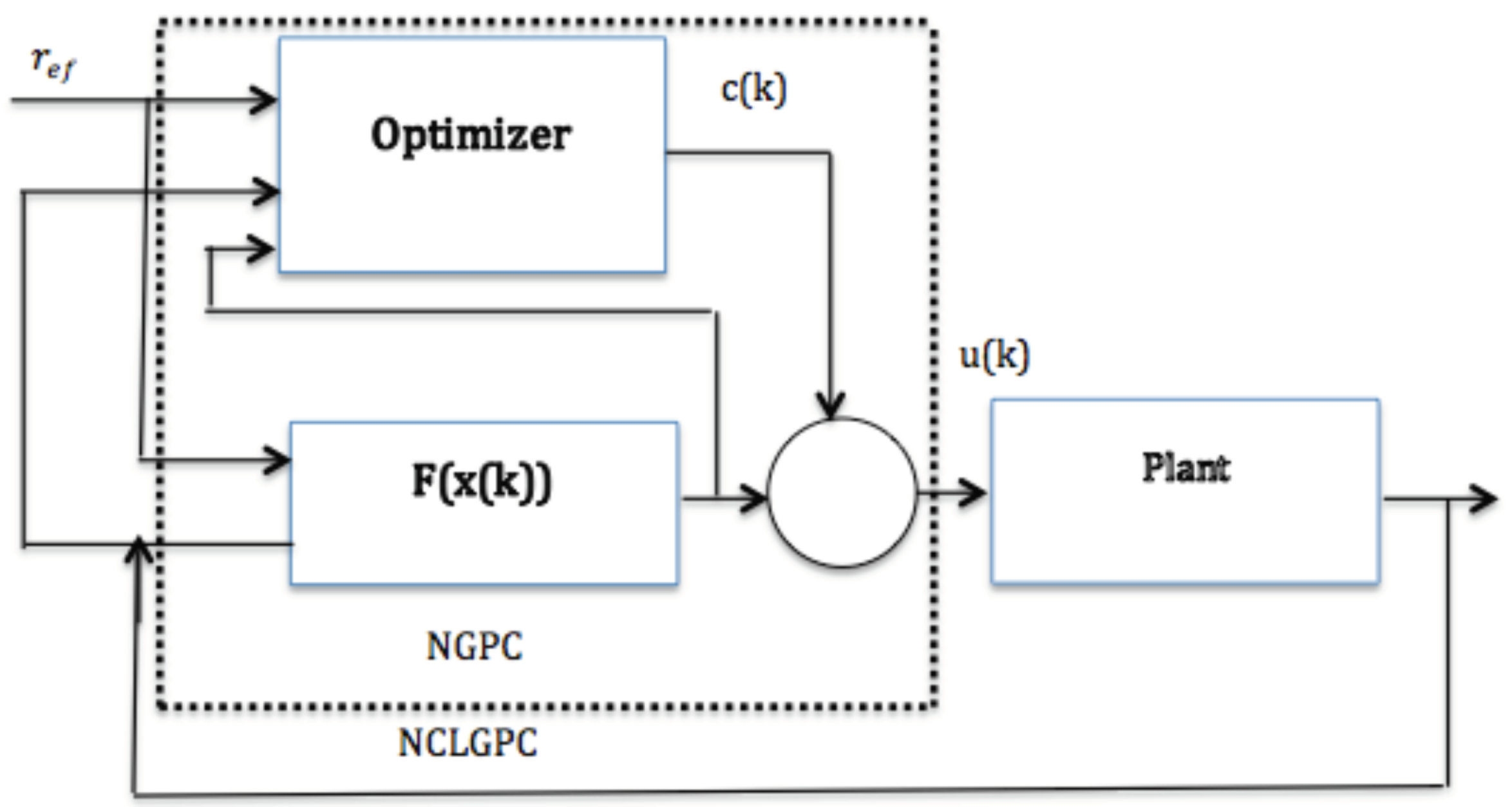
The control strategy proposed in this paper is described schematically in
Figure 1, This controller is achieved by using a new closed loop nonlinear predictive control paradigm that combines an unconstrained economic nonlinear Generalized Predictive Control law
with the parameterization
, associated with the closed loop paradigm that allows taking into account the process constraints and improving the performance of the controller.
Some specific characteristics of this control strategy are:
The optimizer shown in the control scheme (
Figure 1) constitutes the economic nonlinear closed loop paradigm. The predicted control moves are centered around an unconstrained stabilizing control law,
, over the whole prediction horizon, and some additive degrees of freedom,
, are added over a finite horizon to handle constraints. The resulting control
is applied to the plant.
In the objective function the nonlinear economic term is replaced by its gradient making this function a quadratic one.
The prediction model, a nonlinear phenomenological model of the plant, is written as a state dependent coefficient model, also called extended linearization, which consists of factorizing the nonlinear system in a linear structure with state dependent matrices.
The above assumptions allow us to design an economic unconstrained nonlinear GPC analytically, and its stabilizing control law, , and to state the NLCLGPC problem as a QP problem each sampling time.
3. Controller Design
In this section, the Closed Loop Model Predictive Control (CLMPC) that is the basis of the one layer economic controller proposed is presented, starting with the open loop MPC, the predictions using state dependent coefficient matrices and the optimization.
The predictions are obtained using a discrete time varying prediction model of the process along the prediction horizon
of the form:
With initial condition established by:
The predicted input sequences are often stacked into the matrices
defined by:
Clearly
is a function of
, and the optimal input sequence for the problem minimizing
is denoted
:
In order to improve the numerical conditioning of the optimization and the controller performance, a closed loop MPC has been considered by defining the predicted input sequence along the control horizon specified by
as:
where,
is a nonlinear stabilizing state feedback and
.
Then, the predictions considering the closed loop control law are:
The system model becomes
Where is the new manipulated input.
Thus the problem to be minimized at each sampling time is:
where,
and
is the first element of
.
The closed loop nonlinear GPC controller is implemented in a moving horizon framework. At current time step k, the plant state is used as the initial condition and the economic optimization problem is solved on a horizon , however, only the first calculated control action is implemented . At the next time step , we move the time frame one step ahead and the problem is solved with the new plant state as the initial condition.
Remark. - 1.
Due to the non uniqueness of different choices may produce different controllability matrices and one can always find a stabilizable pair . However, although this may be quite easy for lower order systems is becomes laborious for hight order systems.
- 2.
There are numerous ways to choose and the choice of can affect the performance of the controller. Therefore, the non uniqueness of this matrix leads to that the controller developed here is suboptimal rather than optimal.
In the next section, the procedure for obtaining the controller proposed in this work is detailed. First, the analytical solution of the unconstrained economic NLGPC law is computed through the modification of the economic function, later, this law is used to predict the outputs over a prediction horizon with a Nonlinear closed loop Model Predictive Control.
With the aim to integrate RTO with NGPC in one single layer, the inclusion of the gradient of the economic function as an additional term in the cost function is proposed. This approach incorporates the economic objective into the NGPC controller such that the RTO and NGPC are solved in a single optimization routine.
3.1. The Nonlinear GPC with Economic Objective
The objective of this section is to design a nonlinear GPC controller that directly accounts for economic objectives. This is achieved designing a one-layer RTO-GPC controller. To derive the non-linear predictive control algorithm the future trajectory of the system is assumed to be known. State-space model (2) matrices may be re-calculated for the future using the future trajectory. The resulting state-space model may be seen as a time-varying linear model and for this model the controller is designed. In the proposed strategy, due to the presence of
, the objective function Equation (
3) is not a quadratic function of the manipulated variables of the optimization problem that defines the controller. Thus, the control problem turns into an NLP, which may result difficult to solve.
Then, assuming that the vector of the control action is changed to , the first order approximation of the gradient of the economic function
can be represented as follows:
where
corresponds to the process gain.
In the Equation , is the total move of the input vector, D is the gradient vector at the present time and G is the Hessian of the economic function with respect to the inputs. The gradient vector can be considered as a deviation vector, which is equivalent to considering that the gradient of the economic function is zero at the optimum. Thus, can be approximated by a quadratic function as
Remark. In the unconstrained economic optimization, the operating point where the gradient ξ is equal to zero corresponds to a local maximum (when ) or local minimum (when ) of the economic function. However, when the constraints of the control problem are active, the optimum corresponds to the point where the reduced gradient of the economic function is equal to zero. The reduced gradient is obtained through the projection of the gradient on the tangent space of the active constraints.
3.2. NECLGPC Terminal Control Law
In this work, the terminal control law in the NECLGPC is determined online by an unconstrained NGPC Control with finite control and predictions horizons minimizing a cost function constituted by two important terms, the first one for set point tracking and the second for taking into account the economic cost that is approximated by means of its gradient.
The state dependent coefficient form of the model
, in state space format, is stated as in the conventional GPC formulation, allowing for inherent integral action within the model, including the control increment as system input to the state space model. Consequently, an extra system state is incorporated.
where:
Considering that the future trajectory of the state of the system is known, the state-space model matrices may be re-calculated for the future. The resulting state-space model may be seen as a time-varying linear model and the controller is designed using this model. The future trajectory of the system can be determined using this model.
In order to obtain the NGPC control law, the predictive control techniques address calculation of the vector of current and future controls by solving the following optimization problem:
Next the following vectors containing current and future values are introduced:
Then, the cost function
may be written in the vector form:
with
and
.
Now, it is possible to determine the future state prediction:
Note that to obtain the state prediction at time instance the knowledge of matrix predictions and is required. The control increments after the control horizon are assumed to be zero.
Next, the following notation has been introduced:
where
I denotes the identity matrix of appropriate size.
Then
may represented as:
Now using
the following equation for the future state predictions vector
is obtained:
where
From the output Equation it is clear that
Combining the outputs in
and
the following relationship between vectors
and
is obtained:
where
Finally substituting in
by
the following equation for output prediction is obtained:
where
Substituting
in the cost function
by the Equation
and performing the analytical minimization,
is obtained by deriving the cost function:
The Equation
becomes:
3.3. Closed-Loop Paradigm
The dual mode controller proposed in this work differs from others proposed in the literature by three important points. First of all, usually in the classical dual mode MPC schemes, the terminal control law defined in the terminal region is obtained offline by solving a linear quadratic regulator problem, but in this paper the terminal control law is determined online by solving an unconstrained nonlinear GPC problem as presented in the previous paragraph. Secondly, the terminal controller takes into account the economic costs by including the gradient of the economic function as an additional term in the objective function of the NGPC. Finally, here, even though the parameters of NGPC are tuned to assure a good performance and stability if there are not constraints, the dual mode approach is adopted in order to handle constraints when necessary and to the performance of the closed loop system respecting them while maintaining stability.
Remark. It must be stressed that the switching between the modes 1 and 2 in (13) is in the predictions only. The closed loop control law has a single mode, but uses dual mode predictions in the optimization.
A common choice is
as in El bahja, H. [
25] where
F is a unchanging feedback gain computed offline and
is the new manipulated variable. From results of
Section 3.2 and particularly on Equation
, the control parameterization proposed for the CLGPC is based on affine function disturbances as follows, making the controller less conservative.
At each step time k, we assume that the feedback and are constant and is the new decision variable.
The degrees of freedom are the disturbance
as it is described in
Figure 1. It is conventional to define these as:
That is, suppose a limited number of nonzero values for . After the disturbances are zero and the loop acts in a linear fashion and is equivalent to mode 2 of the dual mode predictions. Then the performance index in and constraints , must be formulated in function of .
In order to obtain the prediction equations considering the control parameterization
, those equations are rewritten here:
The predictions with the new control parameterization are:
With and .
Eliminating the dependent variable
one makes:
Predicting onward in time with
one gets;
with
Or in more compact structure we can redact the Equation as
The related input predictions can expressed as
with
or
The state beyond
steps will be denoted as
where
and
are the
block rows of
and
respectively.
3.4. The Algorithm
Steps to follow for design of such controller are summarized in the algorithm below:
- Step 1.
Measure current state vector of the plant (or estimate its value).
- Step 2.
Take the vector calculated in previous iteration and remove the first element , which has already been used in previous iteration for control. Using this vector get the future state predictions .
- Step 3.
Using the predictions and known calculate the future matrix predictions , and for and finally obtain , matrices.
- Step 4.
From calculate and control .
- Step 5.
From calculate and .
- Step 6.
Using the parameterization in and calculate the future vector predictions and by , and .
- Step 7.
Perform the minimization using the future vector predictions obtained in Step 6 and implement , and move on to the next time step.
4. Application to WWTP
Wastewater treatment plants (WWTP) are large nonlinear systems characterized by the complexity of the biological and biochemical phenomena involved. The nonlinear dynamics of the system, the large range of time constants (from a few minutes to several days) observed in the different biological processes and the significant perturbations in the flow and load of the influent make the WWTPs a really challenging case study from the control point of view. The WWTPs have to be operated efficiently, minimizing the energy and recourses consumption while meeting the strict environmental regulations. Therefore, the advanced control strategies as the NLGPC proposed in this paper are a promising alternative for improving their performance and economics.
4.1. Process Model
This application focuses specifically on the N-Removal process, which occurs in the biological treatment of the WWTP. The model that represents the N-Removal process is taken from the Benchmark Simulation Protocol (BSM1) [
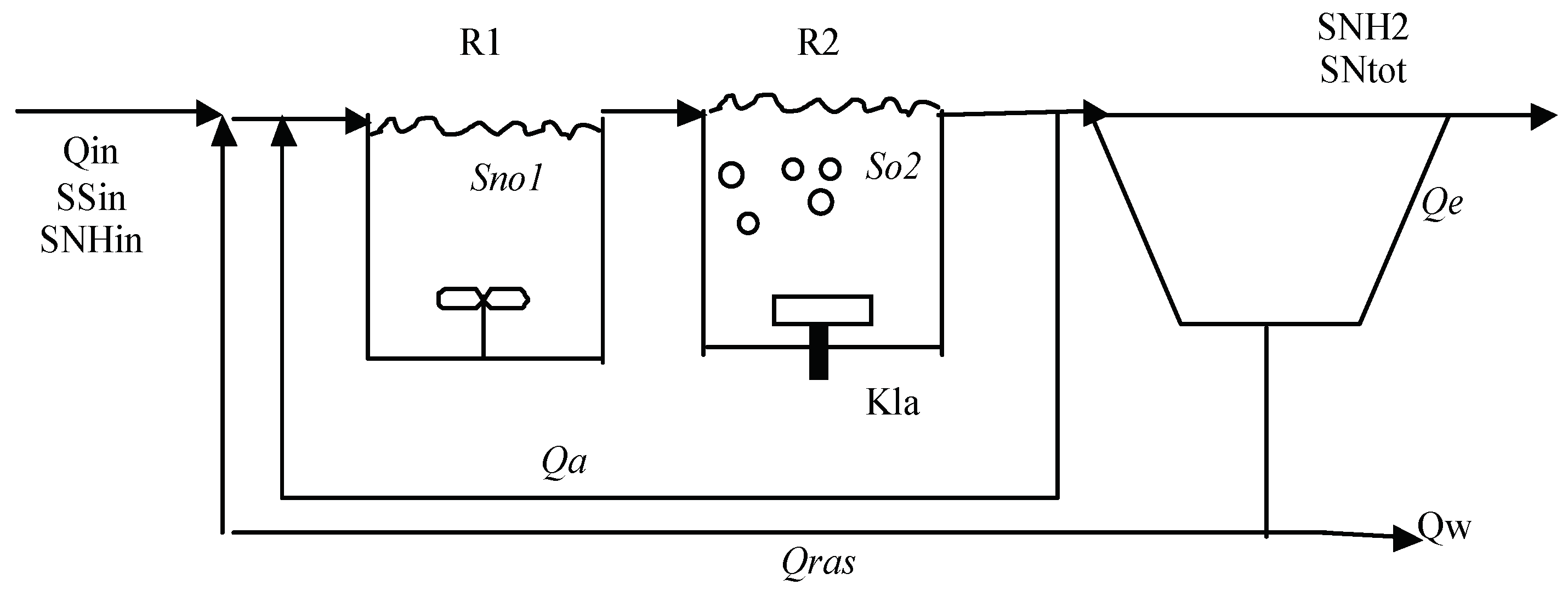
32]. The Benchmark Simulation Model (BSM1) is widely accepted by the scientific community and it has been broadly applied to test control approaches for the Activated Sludge Process (ASP). In order to represent the N-Removal process, the BSM1 is reduced to one anoxic and one aerated reactor, as shown in
Figure 2. The volumes of the tanks are
and
respectively, to make them equivalent to total volumes of the anoxic and the aerobic compartments in the BSM1.
The following equations represent the dynamic behavior of the plant:
In the first reactor, the anoxic growth of heterotrophic biomass is the main biological process, related to denitrification:
In the second reactor, where there is a higher concentration of oxygen, the aerobic growths of heterotrophic and autotrophic biomass are considered, related to nitrification:
The rest of processes are assumed to be zero in Equations and .
The definitions of the state variables are given in
Table 1. The definitions of kinetic and physical parameters are presented in
Table 2 and
Table 3, their values are the same as for BSM1 [
32].
4.2. Operating Conditions
The BSM1 defines the operational requirements of the plant as well as some performance criteria to characterize the effluent quality and the energy consumption [
32]:
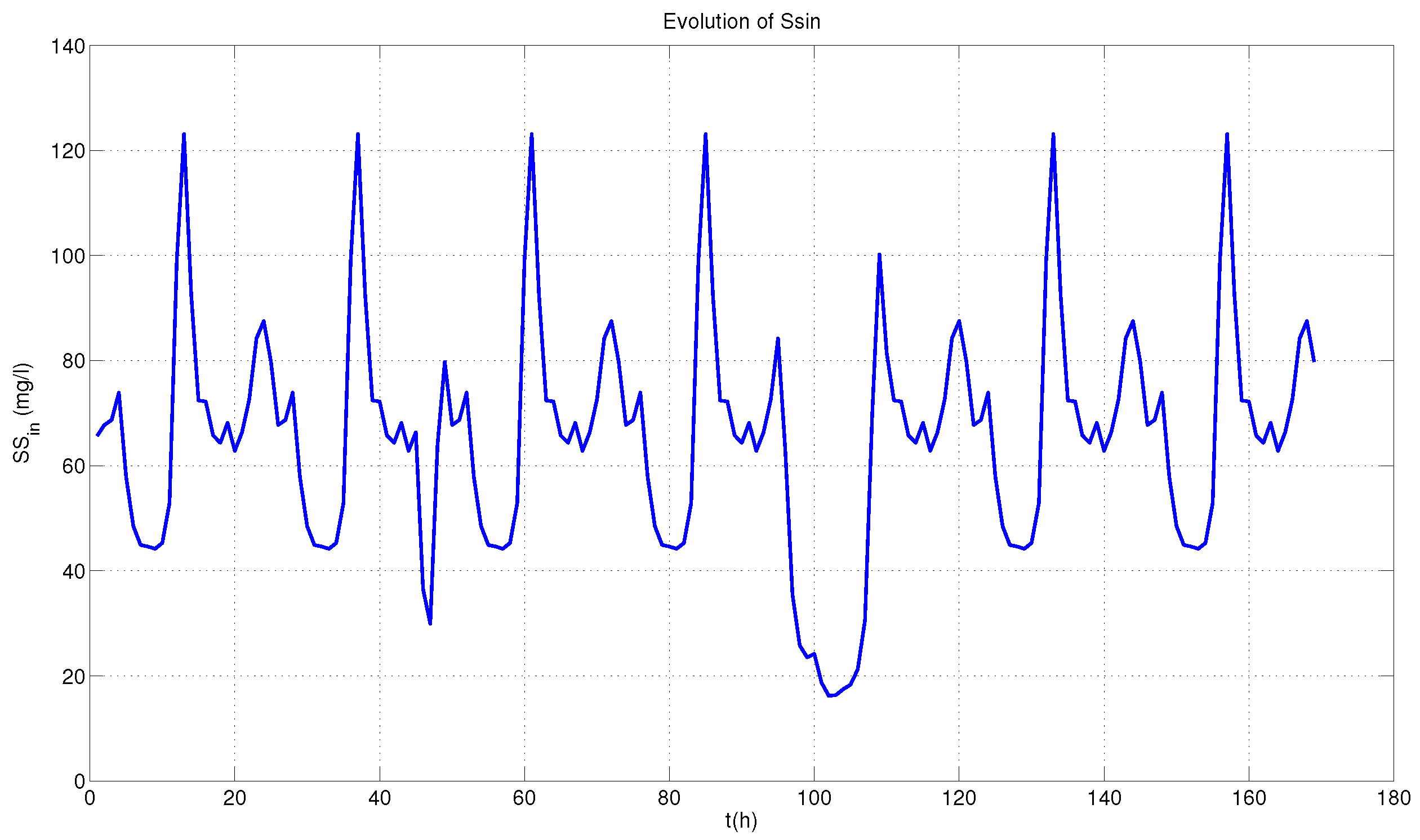
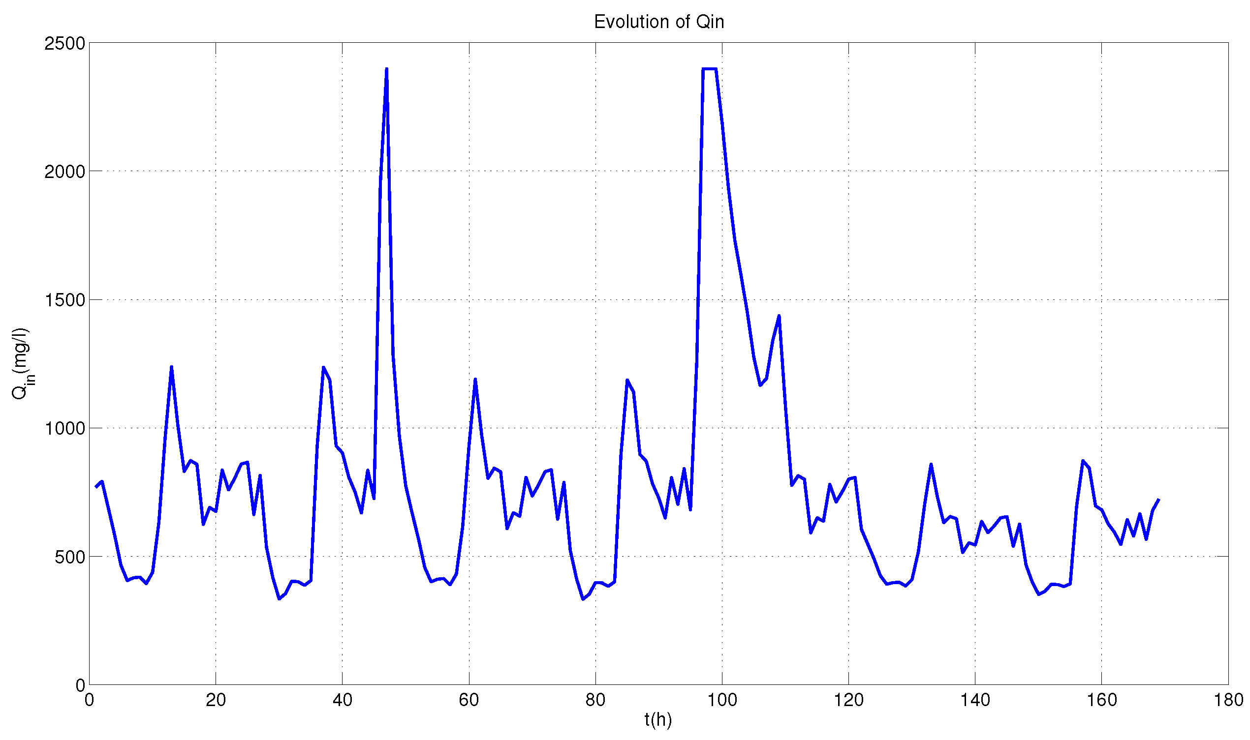
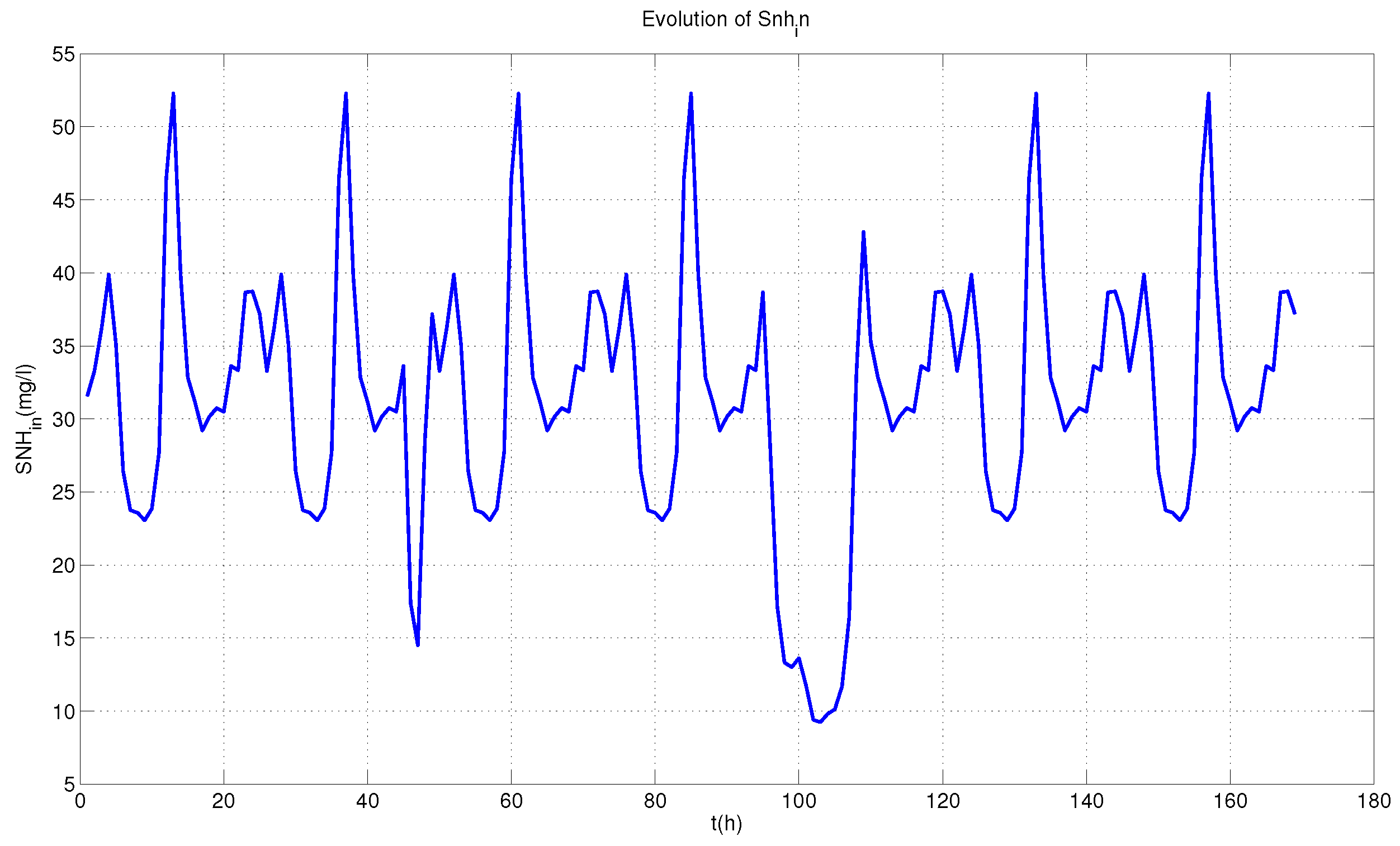
Influent load and disturbances: In order to test the performance of control strategy in different situations, the BSM1 provides standardized influent data considering different weather situations. In this work, data for 336 h, corresponding to 2 weeks starting at time 168 h are considered, with a sampling period of 0.25 h (=15 min) in this work.
Figure 3,
Figure 4 and
Figure 5 present the profiles for stormy weather.
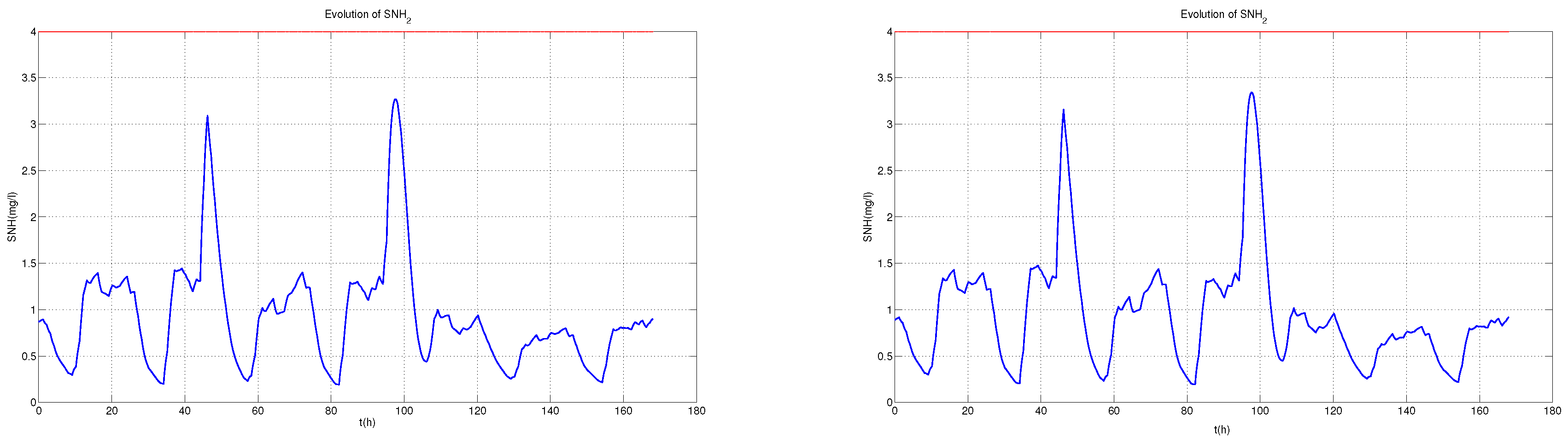
Bounds: The limits on the effluent - ammonium
concentration, total nitrogen
concentration, suspended solid
concentration, biological oxygen demand over a 5-day period
and
are given
Table 4.
Inputs: The two manipulated variables are the internal recycle flow rate and the mass transfer coefficients . The bounds for the input variables are and . The mass transfer coefficient corresponds to the efficiency of the aeration in the aerated tank.
Outputs: The controlled variables are the in the second bioreactor and nitrate levels in the first unit of the bioreactor. Five effluent variables - the ammonium concentration, the concentration of suspended solids, the , the and the total nitrogen - are used to demonstrate the performance of the control system.
4.3. Control problem
The basic control strategy proposed in the is the feedback control of the dissolved oxygen level in the reactor by manipulation of the oxygen transfer coefficient and the control of the nitrites and nitrates concentration in the last anoxic compartment by manipulation of the internal recycle flow rate .
In this work the NECLGPC algorithm is applied for controlling the oxygen
in the aerobic reactor and nitrate levels
in the anoxic reactor. A multivariable control strategy is used where the controlled variables are
and
, the manipulated variables are oxygen transfer coefficient
and the internal recycle flow rate
. The considered measurable disturbances are the influent flow
(
Figure 2), the organic matter concentration
(
Figure 3) and the ammonium concentration
(
Figure 4) in the influent.
4.4. Performance Indices
The measures used to characterize the effluent quality and energy usage during the N-removal process are the standard performance indices recommended in the BSM1 platform for the evaluation of control strategies applied to WWTPs. The Effluent Quality Index () that integrates the total amount of pollutants in the process with different weights depending on their severity, the Aeration Energy () and the Pumping Energy () are applied in this work.
First of all,
(kg pollution/d) is considered as a direct and important indicator of the performance of the control systems as well as the entire wastewater treatment plant. For the BSM1, it is defined as a daily average of a weighted summation of the concentration of different compounds in the effluent over a certain time period as follow:
In the above equation,
denotes total suspended solids and
is the nitrogen total concentration in the effluent. The subscript ’e’ indicates that those concentrations are associated with the effluent of the settler. The weighting factors of
,
and
, and
are adopted from [
32]. The detailed expressions of these variables can be found in [
33]. For the model considered in this work, it is assumed that the separation in the settler produces:
and
.
As for the energy consumption, the total average pumping energy expressed in
(
) over a certain period of time,
T, depends directly on the internal recirculation flaw rate
and it is calculated as [
34]:
where
denotes the return sludge flow rate and
the excess sludge flow rate, both in units of
.
The aeration energy (
) in kWh/d required to aerate the last three comportments can in turn be written as:
where
is the oxygen transfer function in the
kth aerated tank in units of
.
The overall cost index (
) includes the pumping energy (
) and the aeration energy (
) denoted by
:
In the current work, it has been preferred to not work directly with the overall effluent quality index as part of the cost function, because it involves several concentrations not available for measurement. Instead, here, it has been preferred to keep the two main variables of interest (oxygen and nitrate) around desired values, while attempting to keep effluent ammonia under the established limits.
5. Simulations Results
Different advanced control strategies based on nonlinear model predictive control are tested in the WWTP. The idea is to compare the proposed nonlinear GPC proposed in this paper, including the economic term and considering the closed loop paradigm to account for restrictions with other controllers based on GPC that differ in designs and structures.
5.1. Case Studies
Several simulations are carried out to study the process behavior with the different controllers and their effect on process economics and removal efficiency. The performance indices provided by the BSM1 platform are used to evaluate the process performance, with the different controllers in the operating period under characteristic storm weather influent variations. In total five case studies are contemplated in this paper for comparing the control and the performance of the proposed one layer optimizing control strategy. First we present four case studies and then we present another case called case 5 to address the lack of the degree of freedom.
Case 1 (NGPC): Unconstrained Nonlinear Generalized Predictive Control (NGPC) that minimize the following cost function that takes into account only the control objectives, without considering closed loop predictions:
Case 2 (NEGPC): Unconstrained Nonlinear Economic Generalized predictive control (NEGPC) that minimize the following cost function which accounts for economics, but without considering closed loop predictions:
Case 3 (NCLGPC): The one layer optimization and control based on nonlinear closed-loop GPC presented in this work that minimize the following cost function without economics.
Case 4 (NECLGPC): The one layer economic optimization and control based on nonlinear closed-loop GPC presented in this work that minimize the following cost function which accounts for economics.
Those controllers are summarized in the following
Table 5:
Those control strategies are evaluated and compared by means of simulations of the process model (Equations (35)–(42)) implemented in Matlab. The simulations have been carried out considering the influent profile described in
Figure 3,
Figure 4 and
Figure 5 (storm weather scenario), and analogous influents for rain and dry weather described in the BSM1 specifications.
5.2. Tuning Parameters and Operating Conditions
The performance of the plant strongly depends on the selected controller set points due to the plant nonlinearities. The set point selected for the performance evaluation correspond to the economically optimal steady state condition found considering the average values of the inputs in one operating period. The variable
in the second tank is controlled at a set point
and the variable
in the first compartment is controlled at a set point of
. The influent considered has been described in
Figure 3,
Figure 4 and
Figure 5. The plant responses and the corresponding performance indices for 168 (One week) operating hours are compared.
The NECLGPC weights, as well as the prediction and control horizons, affect the closed loop behavior of the plant, so a proper tuning is required. In this work, the tuning has been performed evaluating the plant behavior by means of simulations. The selected tuning parameters for the controllers described in cases 1, 2, 3 and 4 are: control horizon ; prediction horizon ; output weight ; input weight , the weight of the economic term and sampling period of 15 minutes.
The control variables and its rates are bounded as shown in Equations (6) and (9) and therefore, the optimization problem is a nonlinear and constrained. The bounds for the input variables and its rate are , , and .
5.3. Results
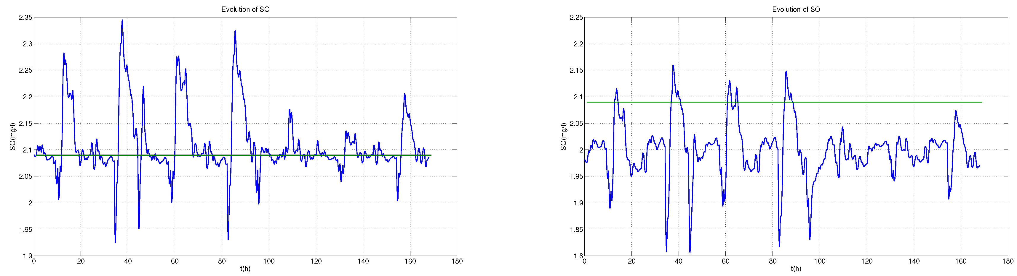
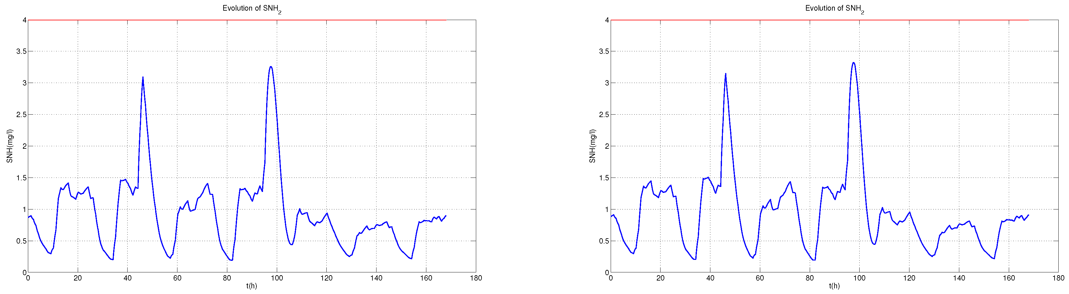
The controller performance evaluation includes the analysis of the temporal responses and the corresponding performance indices. The first comparison is presented in
Figure 6,
Figure 7,
Figure 8 and
Figure 9, where the NGPC (Case 1) is compared to the NEGPC (Case 2), for stormy weather disturbances. For both controllers, the set point tracking is particularly good for the
, and the
concentration satisfies the legal constraint (
Table 4). The responses are very similar, and the only remarkable difference is that for
tracking the NEGPC shows a small offset due to the incorporation of the economic term. The
values (
Table 6) are smaller for NEGPC as expected.
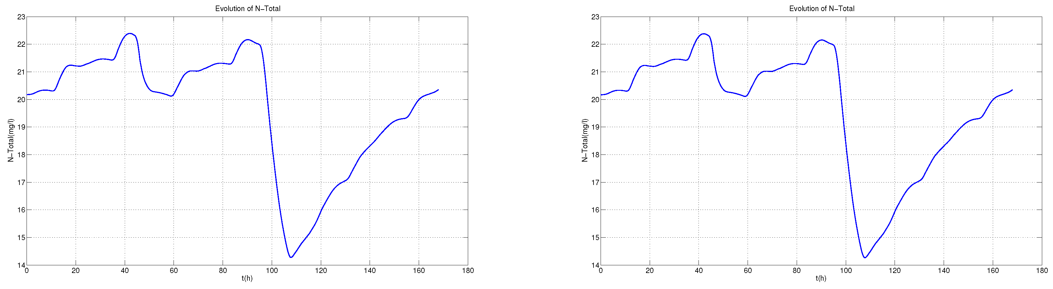
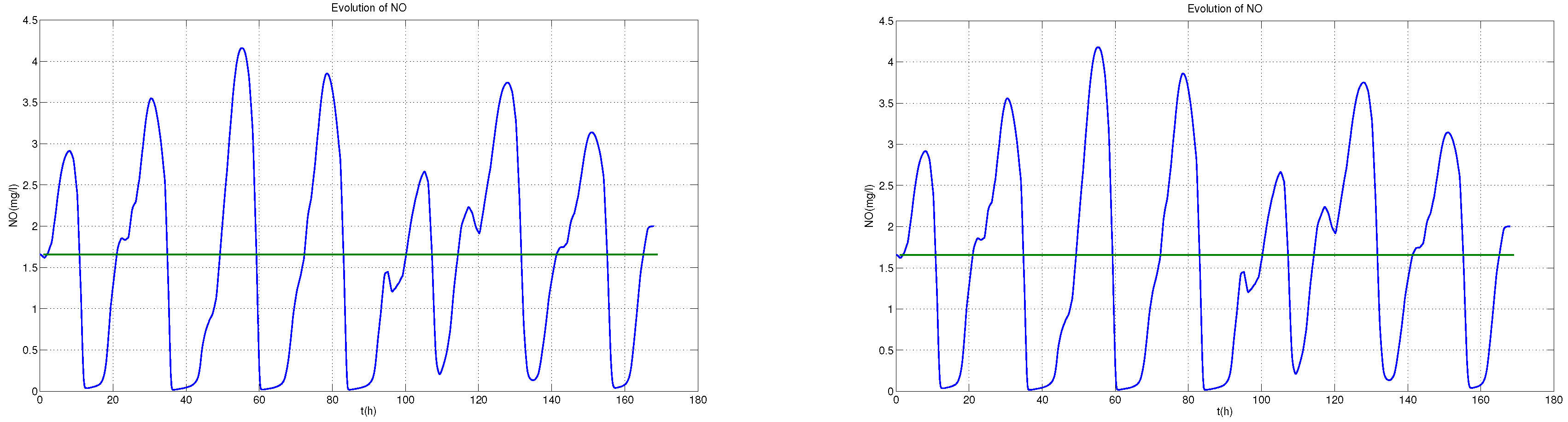
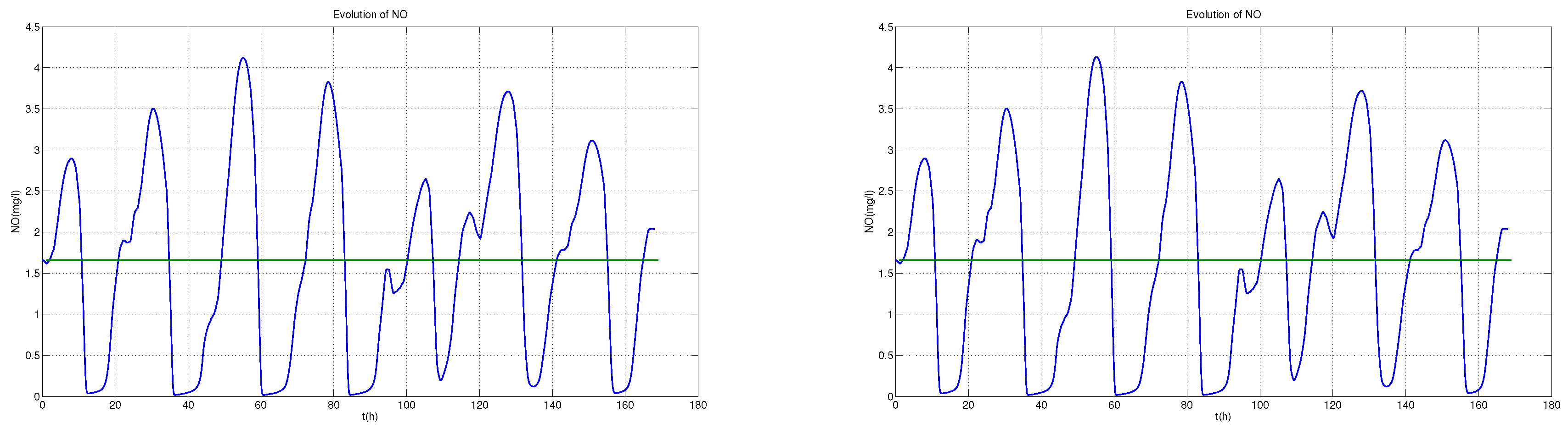
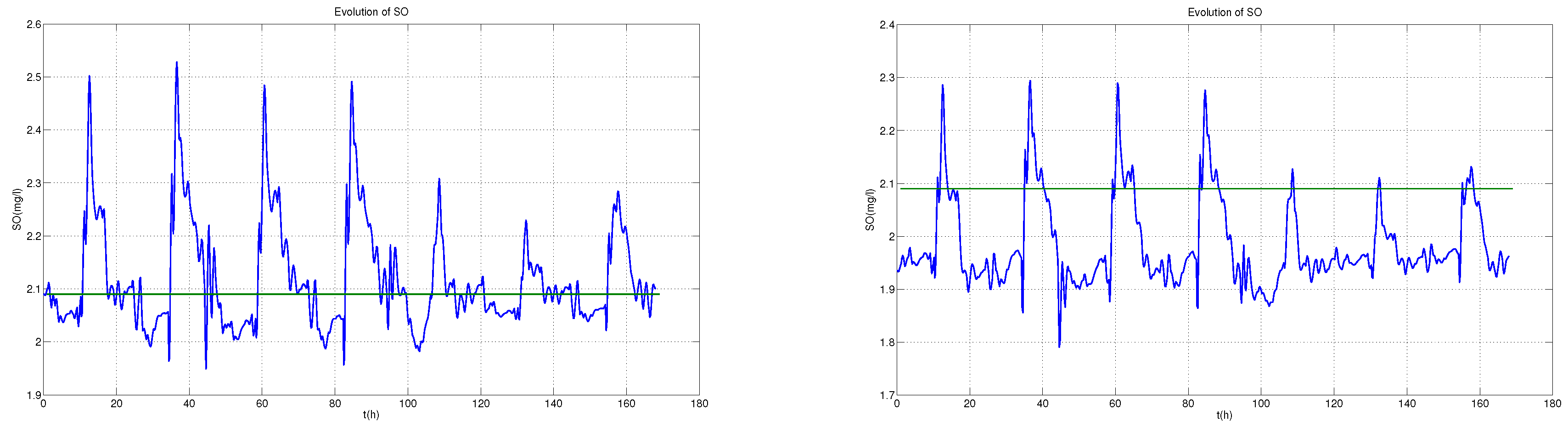
Secondly, in
Figure 10,
Figure 11,
Figure 12,
Figure 13,
Figure 14,
Figure 15 and
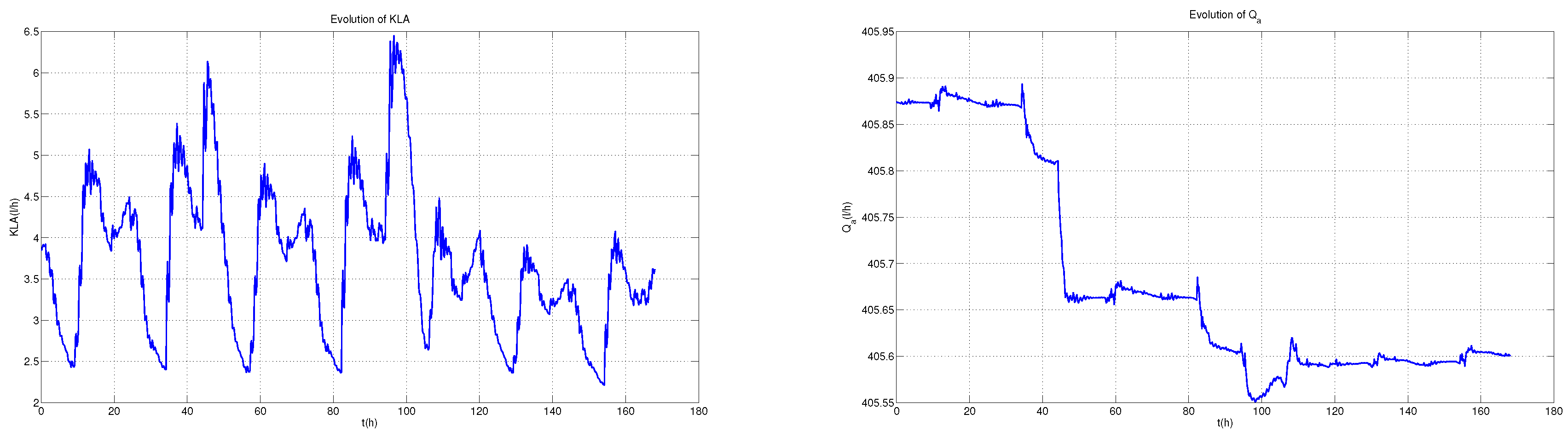
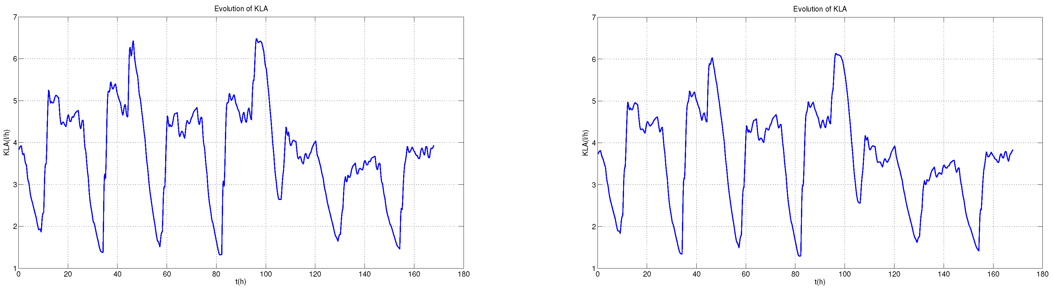
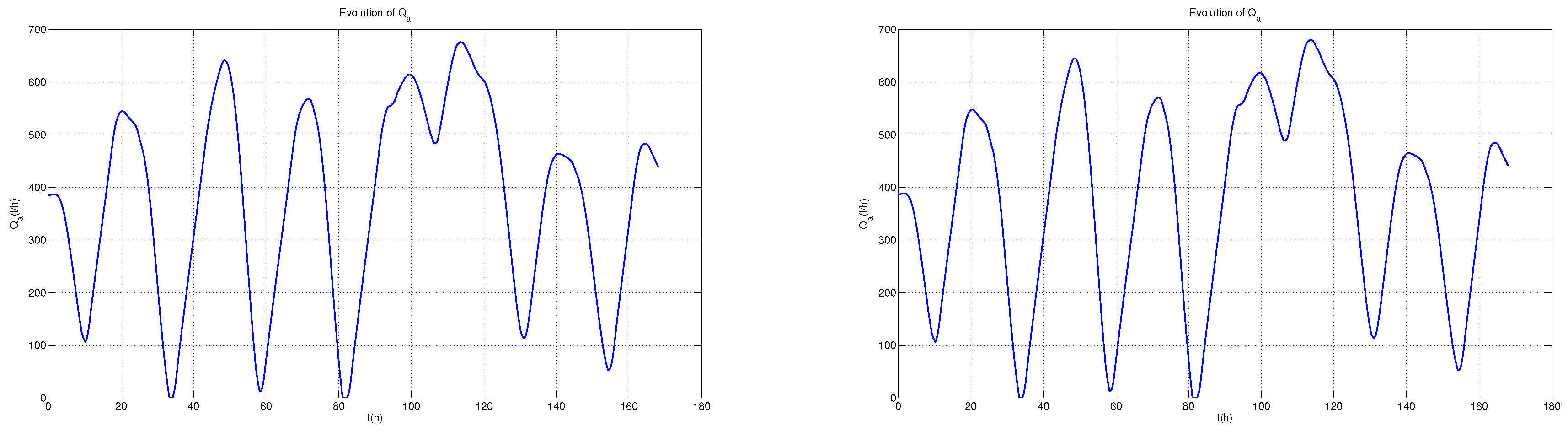
Figure 16 a comparison of the proposed NECLGPC (Case 4) with a NCLGPC (case 3) is presented, also for stormy weather. The responses are again very similar, only showing a small decrease of the manipulated variables for the Case 4 controller, due to the inclusion of the economic term. This is also seen in the
values of
Table 6. For these controllers the tracking for
improves achieving a better balance between
and
tracking. The two manipulated variables are shown in
Figure 12 and
Figure 13 which indicate that suitable control signals
and
drive the process to follow the set point, while satisfying the constraints (Equations (4)–(8)) imposed. The rest of constraints for the effluent (
Table 4) are also satisfied (
Figure 14), ensuring a proper quality of the effluent.
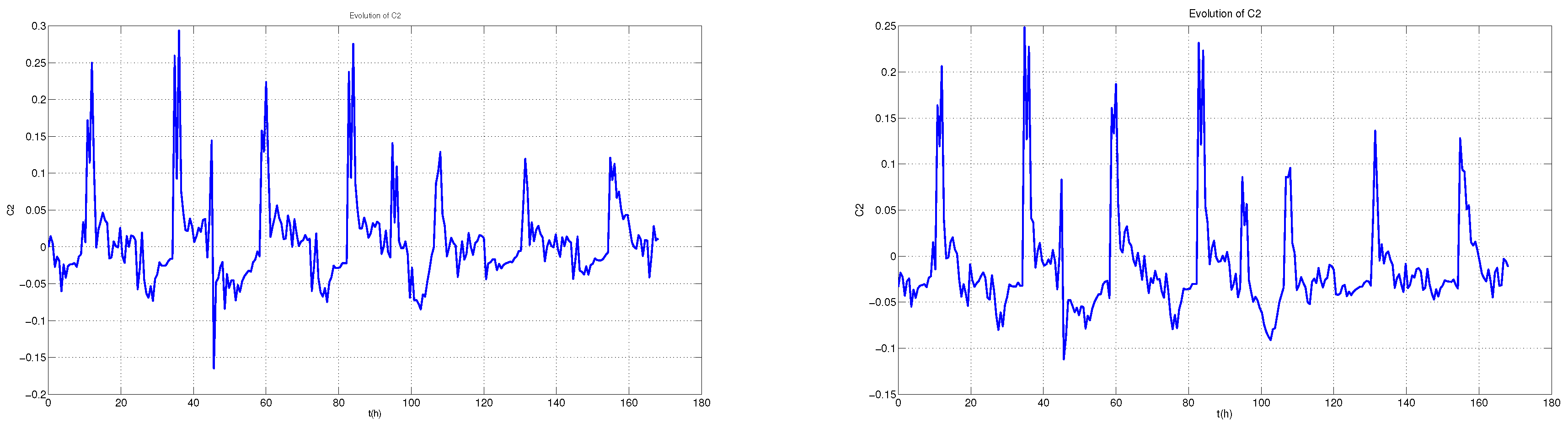
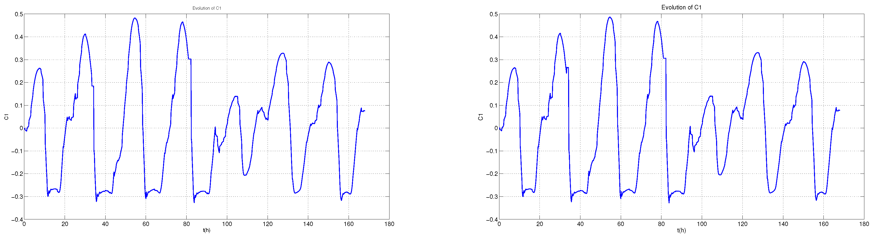
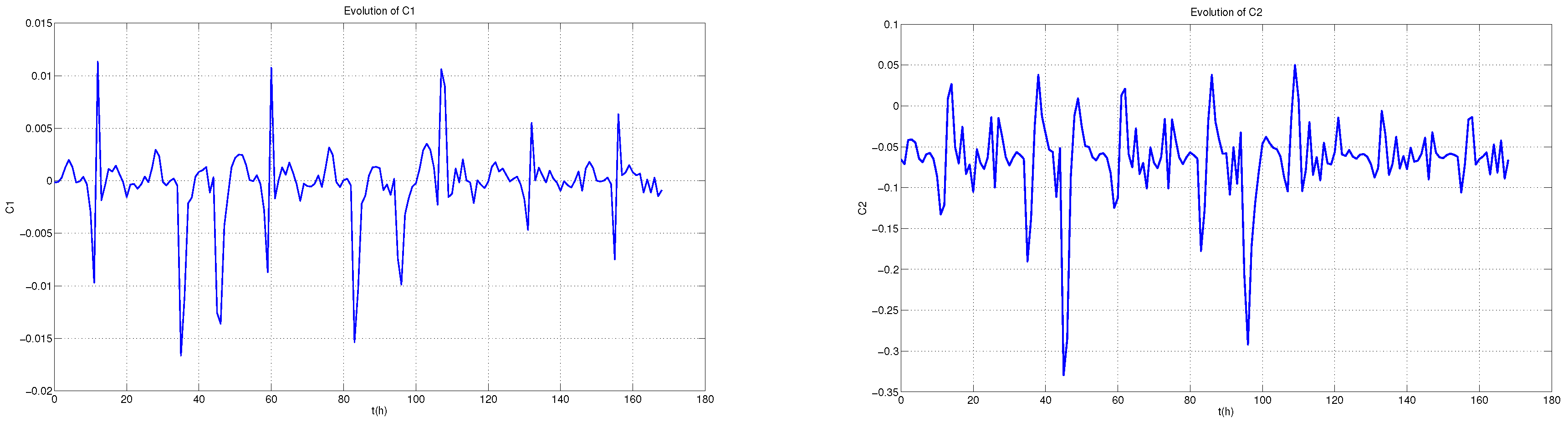
Figure 15 and
Figure 16 show the evolution of the parameters
and
, where can be seen larger variations in
due to the larger variations in
.
In
Table 6, a comparison of different performance indices is shown. Comparing the
for the different case studies, it is possible to observe that the introduction of the economic term in the NECLGPC (case 2) and NEGPC (case 4) improves the economics reducing the
index. For instance, for the storm weather influent it reduces the
from
(Case 1) to
(Case 2) and from
(Case 3) to
(Case 4). This is observed also for different scenarios, especially when dry weather influent profile is tested where a reduction of
of the
is achieved. In order to maintain the controlled variables at the desired reference value, it is necessary to consume energy, which increases the operating costs. Then, the minimization of the pumping energy (PE) and the aeration energy (AE) produce a deviation respect to the desired set point, since not enough freedom degrees are available to meet both requirements at the same time. This deviation is tolerated while the constraints required for the effluent quality are fulfilled.
As general remark, note that there is a small tracking offset in the dissolved oxygen in cases 2 and 3, because of the lack of degree of freedom to minimize costs and perform good tracking simultaneously. In this process there are only two manipulated variables to control two variables and optimize costs.To overcome this problem, either additional degree of freedom could be added by incorporating extra manipulated variables, or a tracking objective can be eliminated, allowing to that variable a free evolution between lower and upper limits.
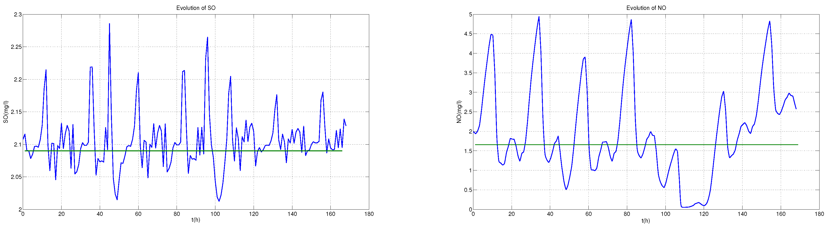
The
Figure 17,
Figure 18 and
Figure 19 presents the case study named case 5, where tracking of NO has been eliminated to leave an additional degree of freedom. A good tracking and disturbance rejection for dissolved oxygen can be seen, while NO has increased its daily variations because
keeps rather constant to decrease costs.
Finally, in
Table 7 a comparison of performance indices is shown, where can be seen that the controller (case 5) provides smaller operating costs than the NCLGPC (case 3), as expected due to the inclusion of a economic cost function in the controller and the new degree of freedom added to allow for cost decrement. As for the EQ index, for both controllers have similar performance, depending on the influent conditions.


