Controllers to Chase a High-Speed Evader Using a Pursuer with Variable Speed

Abstract

This paper proposes a chasing controller to enable a pursuer to chase a high-speed evader such that the relative distance between the evader and the pursuer monotonically decreases as time passes. Our controller is designed to assure that the angular rate of Line-of-Sight joining the pair (the pursuer and the evader) is exactly zero at all time indexes. Assuming that the pursuee can readily observe optical flow, but only poorly detect looming, this pursuer’s movement is hardly detected by the pursuee. Consider the terminal phase when the pursuer is sufficiently close to the evader. As we slow down the relative speed of the pursuer with respect to the evader, we can reduce the probability of missing the high-speed evader. Thus, our strategy is to make the pursuer decrease its speed in the terminal phase, while ensuring that the distance between the evader and the pursuer monotonically decreases as time passes. The performance of our controller is verified utilizing MATLAB simulations.

1. Introduction

This paper proposes a chasing controller so that a pursuer can chase and capture a maneuvering evader which moves at high speed. This problem is related to the challenging missile guidance problem of intercepting a high-speed missile [1,2,3,4,5,6]. The pursuer must move at high speed to capture a high-speed evader. Consider the terminal phase when the pursuer is sufficiently close to the high-speed evader. The accurate control of the pursuer in the terminal phase is crucial, since it is hard to capture a high-speed evader if the pursuer misses the evader in the terminal phase.

Our strategy in the terminal phase is to slow down the pursuer’s speed. As we slow down the relative speed of the pursuer with respect to the evader, we can decrease the probability of missing the high-speed evader. (Consider the case where two spaceships dock each other. It is desirable to slow down the relative speed for safe and accurate docking). Thus, our strategy is to make the pursuer decrease its speed in the terminal phase, while ensuring that the distance between the evader and the pursuer monotonically decreases as time passes. As far as we know, no paper in the literature on chasing targets considered changing the pursuer’s speed so as to capture a maneuvering evader in a provably complete manner.

Our controller is designed to assure that the angular rate of Line-of-sight joining the pair (the pursuer and the evader) is exactly zero at all time indexes. This type of movement is called the motion camouflage with respect to a fixed point at infinity [7,8,9].

This motion camouflage is employed by various visual insects and animals to achieve prey capture, mating, or territorial combat [8,10,11,12]. This movement is a time-optimal solution to capture a pursuee moving with a constant velocity (speed and heading) [10]. In addition [10], argued that this motion minimizes time-to-capture of an unpredictably moving pursuee. Assuming that the pursuee can readily observe optical flow, but only poorly detect looming, this pursuer’s movement is hardly detected by the prey [8].

This paper introduces a chasing controller to enable a pursuer to chase a maneuvering evader while not rotating the LOS joining the pair (the evader and the pursuer). We make the pursuer decrease its speed in the terminal phase, while ensuring that the distance between the evader and the pursuer monotonically decreases as time passes.

The literature is abundant with papers on planning path of robots [8,13,14,15,16,17,18,19,20,21,22,23,24,25,26,27]. Kim [28] developed a path planning algorithm for an underwater robot approaching a static target while not being detected by the target. The path was planned to reduce both the time required to meet the target and the robot’s sound measured by the static target.

The authors of [29,30,31] presented the autonomous tracking and following of a marine vessel by an Unmanned Surface Vehicle (USV) in the presence of dynamic obstacles. In [29,30], the path planning for the USV with International Regulations for Preventing Collisions at Sea (COLREGS) rules was achieved. The authors of [31] presented a trajectory planning and tracking approach for following a differentially constrained target vehicle operating in an obstacle field. Svec [31] predicted the target state several time steps forward in time and generated a collision-free trajectory to allow the USV to safely reach the predicted target state. As far as we know, no paper on chasing targets handled changing the pursuer’s speed so as to capture a maneuvering evader in a provably complete manner.

Many controllers have been developed to mimic motion camouflage in nature. To capture an evader [7,8,9,32] presented a chasing controller based on biologically plausible sensing. Galloway and Raju [9,32] developed a motion camouflage controller in noisy environments. Note that [7,8,9] only considered a pursuer which moves with a constant speed.

As missile controllers, Proportional Navigation Guidance (PNG) controls and their variations were widely used to let the pursuer capture the evader [1,3,4,5,6]. PNG laws enable the pursuer to capture the evader by driving the angular rate of LOS near zero as time passes [4]. But, PNG laws do not make the angular rate of LOS stay at zero at every time index. Note that PNG laws only considered a pursuer which moves with a constant speed.

This paper proves that utilizing our chasing controller, the distance between the evader and the pursuer monotonically decreases, regardless of evader’s maneuver or acceleration, if the following assumptions are satisfied: (1) the pursuer speed is bigger than the evader speed; (2) the pursuer can predict the evader’s location within two time steps in the future.

Our controller works as follows. The locations of both the pursuer and the evader are accessed at every time index. Considering a robot control system, the location of the pursuer is estimated in real time, since a robot (pursuer) can access the movement of itself utilizing Inertial Navigation Sensor (INS) or Global Positioning System (GPS). The pursuer uses sensor measurements, such as radar, to measure the evader’s location in real time.

Based on the accessed evader locations, the pursuer predicts the evader’s location two steps forward in time. We acknowledge that sensor measurement noise exists as the pursuer measures the evader’s location in real time. Moreover, predicted evader location is related to evader maneuvers and is not easy to conjecture in an accurate manner. The effect of prediction error on the performance of our motion camouflage controller is analyzed in Section 4.2.

Since the maximum acceleration of the evader is bounded, we can assume that the evader’s motions are smooth, so the evader’s trajectory curves are derivative. Under this assumption, Section 4 presents a fitting method to predict the evader’s location two steps forward in time.

After predicting the evader’s location two steps forward in time, the pursuer calculates its velocity command, while ensuring that the LOS does not rotate at the next time index. Using deduction, the angular rate of LOS is zero at every time index. In Section 5, the effectiveness of our chasing controller is demonstrated utilizing MATLAB simulations.

This paper is organized as follows. Section 2 presents several definitions and assumptions before presenting our main results. Section 3 presents our chasing controller. Section 4 presents a method to predict the evader location two steps forward in time considering noisy environments. Section 5 introduces MATLAB simulation results to demonstrate the performance of our chasing controller. Section 6 provides Conclusions.

2. The Assumptions and Definitions

2.1. Definitions

Several definitions and assumptions are introduced before presenting our main results. $\angle ({\mathbf{v}}_1,{\mathbf{v}}_2)$ is the angle formed by two vectors ${\mathbf{v}}_1$ and ${\mathbf{v}}_2$. Mathematically, $\angle ({\mathbf{v}}_1,{\mathbf{v}}_2)=arccos(\frac{{\mathbf{v}}_1·{\mathbf{v}}_2}{\parallel {\mathbf{v}}_1\parallel \parallel {\mathbf{v}}_2\parallel })$. Here, $\angle ({\mathbf{v}}_1,{\mathbf{v}}_2)$ exists between 0 and $\pi$. T is the sampling interval of our chasing controller in discrete-time systems.

${\mathbf{r}}_k^e$ is the evader’s location at time index k. ${\mathbf{r}}_k^p$ is the pursuer’s location at time index k. The pursuer is in the motion camouflage state at time index $k+1$ in the case where $\angle ({\mathbf{r}}_{k+1}^p-{\mathbf{r}}_{k+1}^e,{\mathbf{r}}_k^p-{\mathbf{r}}_k^e)=0$.

$v_k^p$ is the pursuer’s speed at time index k. $v_k^e$ is the evader’s speed at time index k. The subscript k implies the time index k.

The pursuer’s motion model is

$$\begin{array}{c}\hfill {\mathbf{r}}_{k+1}^p={\mathbf{r}}_k^p+T{v}_k^p{\mathbf{u}}_k.\end{array}$$

(1)

Here, ${\mathbf{u}}_k$ is a unit vector and indicates the pursuer’s heading at time index k. ${\mathbf{u}}_k$ is determined at every time index k so that the pursuer is in the motion camouflage state at time index k.

In addition, the evader’s motion model is

$$\begin{array}{c}\hfill {\mathbf{r}}_{k+1}^e={\mathbf{r}}_k^e+T{\mathbf{v}}_k^e.\end{array}$$

(2)

Here, ${\mathbf{v}}_k^e$ indicates the evader’s velocity vector at time index k.

In order to capture the evader, it is necessary that the evader’s speed is slower than the pursuer’s speed ([1,2] introduced a variation of PNG controls to capture evaders that are of higher speeds than the pursuer. But, considering a high-speed evader which moves away from a slowly moving pursuer, it is impossible to capture the evader). We control the pursuer’s speed so that it is always bigger than that of the evader. This implies that $v_k^e<v_k^p$ at every time index k.

Let $a_m$ denote the pursuer’s maximum acceleration. In addition, let $ϵ>0$ denote a small constant. The required time interval to decrease the pursuer’s speed from $v_k^p$ to $v_k^e+ϵ$ is

$$\begin{array}{c}\hfill T_r=(v_k^p-v_k^e-ϵ)/a_m.\end{array}$$

(3)

The traversal distance of the pursuer as it decreases its speed from $v_k^p$ to $v_k^e+ϵ$ is

$$\begin{array}{c}\hfill D_k=v_k^p\ast T_r-0.5\ast a_m\ast T_r\ast T_r.\end{array}$$

(4)

We say that the pursuer is in the terminal phase in the case where

$$\begin{array}{c}\hfill \parallel {\mathbf{r}}_k^e-{\mathbf{r}}_k^p\parallel <D_k.\end{array}$$

(5)

is met.

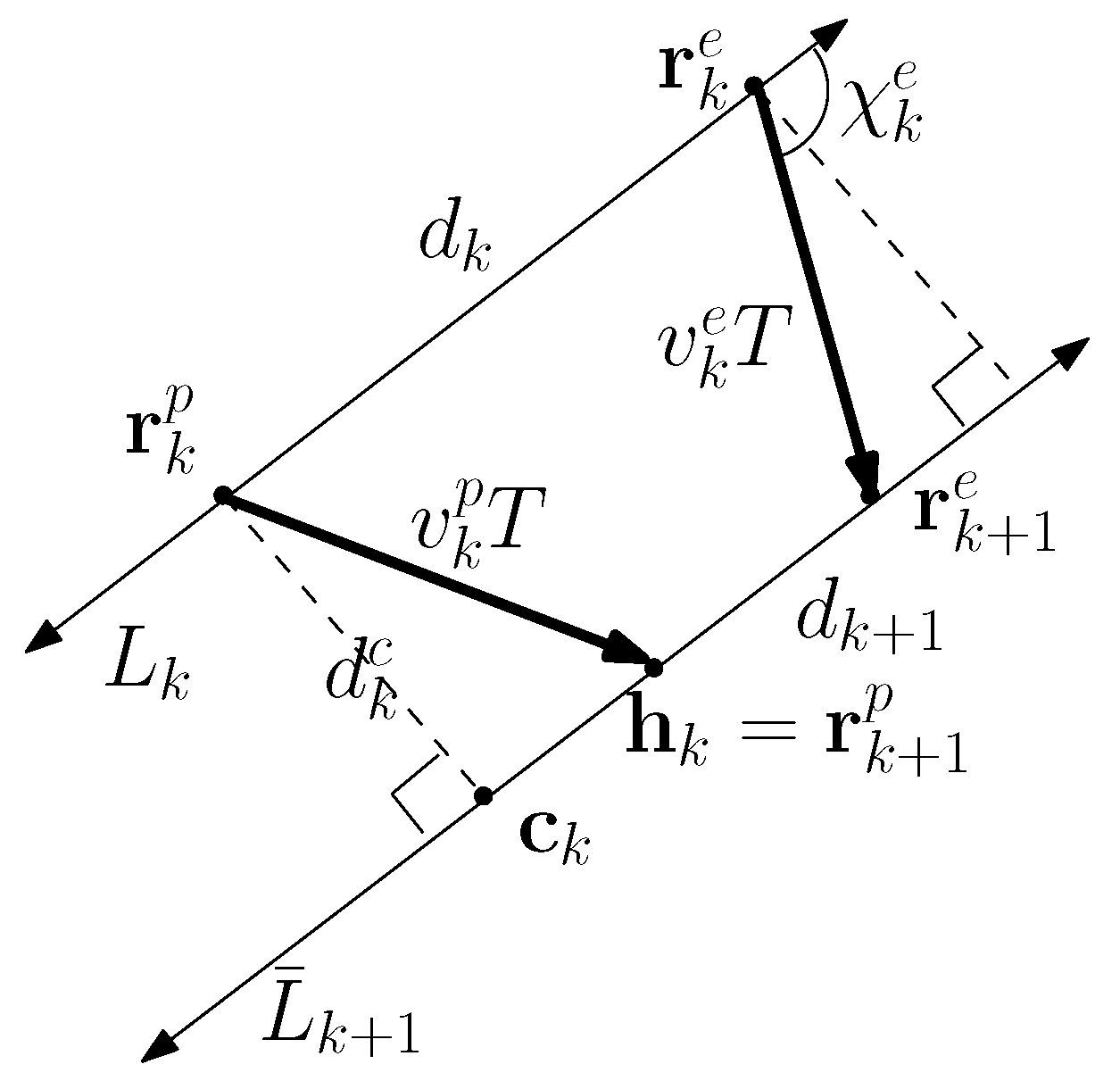
$L_k$ is the infinite line (LOS) intersecting both ${\mathbf{r}}_k^p$ and ${\mathbf{r}}_k^e$. We draw one infinite line (LOS) ${\overline{L}}_{k+1}$ intersecting ${\mathbf{r}}_{k+1}^e$, such that ${\overline{L}}_{k+1}$ is parallel to $L_k$. Note that there exists only one infinite line intersecting ${\mathbf{r}}_{k+1}^e$, such that the line is parallel to $L_k$.

${\mathbf{c}}_k$ is the point on ${\overline{L}}_{k+1}$, which is the closest to ${\mathbf{r}}_k^p$. Let $d_k^c=\parallel {\mathbf{r}}_k^p-{\mathbf{c}}_k\parallel$, and let ${\chi }_k^e=\angle ({\mathbf{r}}_k^e-{\mathbf{r}}_k^p,{\mathbf{r}}_{k+1}^e-{\mathbf{r}}_k^e)$. Let $d_k=\parallel {\mathbf{r}}_k^p-{\mathbf{r}}_k^e\parallel$. See Figure 1 for an illustration of these concepts.

As depicted in Figure 1, $d_k^c=v_k^{e}Tsin({\chi }_k^e)\le v_k^{e}T$. Since $v_k^e<v_k^p$, we have

$$\begin{array}{c}\hfill d_k^c<v_k^{p}T.\end{array}$$

(6)

Utilizing (6), we define ${\delta }_k>0$ as follows.

$$\begin{array}{c}\hfill {\delta }_k=\sqrt{{(v_k^{p}T)}^2-{(d_k^c)}^2}.\end{array}$$

(7)

We also define the heading point ${\mathbf{h}}_k$ as follows:

$$\begin{array}{ccc}\hfill {\mathbf{h}}_k& =& {\mathbf{c}}_k+\frac{{\mathbf{r}}_k^e-{\mathbf{r}}_k^p}{\parallel {\mathbf{r}}_k^e-{\mathbf{r}}_k^p\parallel }{\delta }_k.\hfill \end{array}$$

(8)

Here, ${\delta }_k$ satisfies that $\parallel {\mathbf{h}}_k-{\mathbf{r}}_k^p\parallel$ is $v_k^{p}T$. See Figure 1.

At every time index k, the pursuer heads towards the heading point ${\mathbf{h}}_k$. Consider a circle centered at ${\mathbf{r}}_k^p$, whose radius is $v_k^{p}T$. Due to (6), ${\overline{L}}_{k+1}$ intersects this circle at two points. Between these two points, the heading point ${\mathbf{h}}_k$ is the point which is the closest to ${\mathbf{r}}_{k+1}^e$. This way, the pursuer maneuvers to decrease the distance between the pursuer and the evader, while not rotating the LOS.

Let us draw both x-axis and y-axis satisfying the following conditions:

• Both x-axis and y-axis are normal to each other, and they intersect at ${\mathbf{c}}_k$. ${\mathbf{c}}_k$ is set as the origin.
• the coordinate of ${\mathbf{r}}_{k+1}^p={\mathbf{h}}_k$ is $({\delta }_k,0)$.
• The coordinate of ${\mathbf{r}}_k^p$ is $(0,d_k^c)$.

First, we handle the case where ${\chi }_k^e>\pi /2$. This case, the evader maneuvers to decrease the distance between the pursuer and the evader. Utilizing the geometry in Figure 1, the coordinate of ${\mathbf{r}}_{k+1}^e$ is

$$\begin{array}{c}\hfill {co}_1({\mathbf{r}}_{k+1}^e)=(d_k-{\alpha }_k,0).\end{array}$$

(9)

Here, ${\alpha }_k=\sqrt{{(v_k^{e}T)}^2-{(d_k^c)}^2}$ is positive.

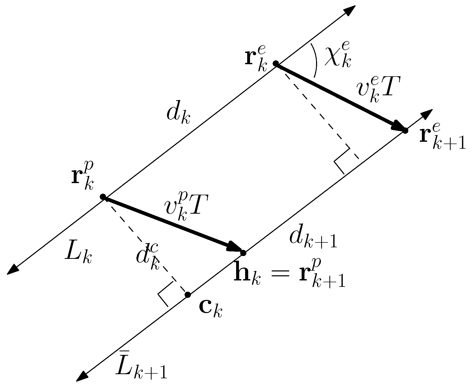
Next, we handle the case where ${\chi }_k^e\le \pi /2$. This case, the evader maneuvers to increase the distance between the pursuer and the evader. Utilizing the geometry in Figure 2, the coordinate of ${\mathbf{r}}_{k+1}^e$ is

$$\begin{array}{c}\hfill {co}_2({\mathbf{r}}_{k+1}^e)=(d_k+{\alpha }_k,0).\end{array}$$

(10)

2.2. Assumptions

In this paper, we assume that the pursuer’s location is estimated in real time. In addition, the pursuer can estimate the evader’s location at every time index. Therefore, the pursuer can access $L_k$ at every time index k. Since the maximum acceleration of the evader is bounded, we assume that the evader’s motions are smooth, so the evader’s trajectory curves are derivative. We further assume that the pursuer can predict the evader’s location two steps forward in time, which implies that the pursuer at time index k can estimate the evader’s velocities ${\mathbf{v}}_k^e$ and ${\mathbf{v}}_{k+1}^e$.

3. Control Law

We introduce how to control the pursuer’s speed. We assumed that the pursuer at time index k can estimate the evader speed $v_k^e$. $v_k^p$ can change with respect to k as long as

$$\begin{array}{c}\hfill v_k^p>v_k^e\end{array}$$

(11)

is met at each time step k.

Our strategy in the terminal phase is to slow down the pursuer’s speed as long as (11) is met. This implies that in the terminal phase, we update the pursuer’s speed using

$$\begin{array}{c}\hfill v_{k+1}^p=max(v_k^p-a_{m}T,v_{k+1}^e+ϵ).\end{array}$$

(12)

Here, $ϵ>0$ is a small constant. Note that $v_{k+1}^e$ is available, since the pursuer at time index k can estimate the evader’s velocities ${\mathbf{v}}_k^e$ and ${\mathbf{v}}_{k+1}^e$. (12) implies that (11) is met at each time step.

We next introduce the heading control ${\mathbf{u}}_k$ to achieve motion camouflage. ${\mathbf{u}}_k$ is chosen so that the pursuer moves to ${\mathbf{h}}_k$. At every time index k, the heading controller is given as follows. At every time index k, the pursuer selects the new heading command ${\mathbf{u}}_k$ as $\frac{{\mathbf{h}}_k-{\mathbf{r}}_k^p}{\parallel {\mathbf{h}}_k-{\mathbf{r}}_k^p\parallel }$.

Consider the situation where the distance between ${\mathbf{r}}_k^p$ and ${\mathbf{r}}_{k+1}^e$ is less than $v_k^{p}T$. In this situation, the pursuer moves towards ${\mathbf{r}}_{k+1}^e$ directly, while not using ${\mathbf{u}}_k=\frac{{\mathbf{h}}_k-{\mathbf{r}}_k^p}{\parallel {\mathbf{h}}_k-{\mathbf{r}}_k^p\parallel }$. In this way, the evader is captured at time index $k+1$.

In practice, the pursuer cannot turn with infinite acceleration. Suppose that the maximum turn rate of the pursuer is q radians per second. In the case where the angle formed by ${\mathbf{u}}_{k-1}$ and the new heading command, $\frac{{\mathbf{h}}_k-{\mathbf{r}}_k^p}{\parallel {\mathbf{h}}_k-{\mathbf{r}}_k^p\parallel }$, is bigger than $qT$ radians, then the heading command $\frac{{\mathbf{h}}_k-{\mathbf{r}}_k^p}{\parallel {\mathbf{h}}_k-{\mathbf{r}}_k^p\parallel }$ cannot be achieved within one sampling interval. This case, we select ${\mathbf{u}}_k$ using the following method.

Let ${\mathbf{u}}_k^1=\mathbf{R}(qT){\mathbf{u}}_{k-1}$, where $\mathbf{R}(qT)=\left(\begin{array}{cc}cos(qT)& sin(qT)\\ -sin(qT)& cos(qT)\end{array}\right)$. In addition, let ${\mathbf{u}}_k^2=\mathbf{R}(-qT){\mathbf{u}}_{k-1}$. If $\parallel \frac{{\mathbf{h}}_k-{\mathbf{r}}_k^p}{\parallel {\mathbf{h}}_k-{\mathbf{r}}_k^p\parallel }-{\mathbf{u}}_k^1\parallel <\parallel \frac{{\mathbf{h}}_k-{\mathbf{r}}_k^p}{\parallel {\mathbf{h}}_k-{\mathbf{r}}_k^p\parallel }-{\mathbf{u}}_k^2\parallel$, then we set ${\mathbf{u}}_k={\mathbf{u}}_k^1$. Otherwise, we set ${\mathbf{u}}_k={\mathbf{u}}_k^2$. In this manner, the heading command ${\mathbf{u}}_k$ can be achieved within one sampling interval.

In the following sections associated with analysis (Section 3.1, Section 3.2, and Section 4), it is assumed that $q=inf$. This implies that we analyze the performance of our chasing controller, not considering the maximum turn rate of the pursuer. In the Simulation section, we set $q=\pi /6$ radians per second.

3.1. Stability Analysis

Next, the stability of our chasing controller is analyzed. It is derived that $\angle ({\mathbf{r}}_{k+1}^p-{\mathbf{r}}_{k+1}^e,{\mathbf{r}}_k^p-{\mathbf{r}}_k^e)=0$ at every time index $k>1$ under our chasing controller. This implies that the motion camouflage state is achieved at every time index $k>1$.

Theorem 1.

Under our heading controller ${\mathbf{u}}_k$, $\angle ({\mathbf{r}}_{k+1}^p-{\mathbf{r}}_{k+1}^e,{\mathbf{r}}_k^p-{\mathbf{r}}_k^e)=0$ at every time index $k>1$.

Proof. 

At every time index k, the pursuer sets ${\mathbf{u}}_k$ as $\frac{{\mathbf{h}}_k-{\mathbf{r}}_k^p}{\parallel {\mathbf{h}}_k-{\mathbf{r}}_k^p\parallel }$. Utilizing the pursuer’s motion model in (1), we further get

$$\begin{array}{c}\hfill {\mathbf{r}}_{k+1}^p={\mathbf{r}}_k^p+\frac{{\mathbf{h}}_k-{\mathbf{r}}_k^p}{\parallel {\mathbf{h}}_k-{\mathbf{r}}_k^p\parallel }{v}_k^{p}T.\end{array}$$

(13)

The heading point ${\mathbf{h}}_k$ is set utilizing (8). In (8), ${\delta }_k$ satisfies that $\parallel {\mathbf{h}}_k-{\mathbf{r}}_k^p\parallel$ is $v_k^{p}T$. By substituting $\parallel {\mathbf{h}}_k-{\mathbf{r}}_k^p\parallel$ in (13) for $v_k^{p}T$, we obtain

$$\begin{array}{c}\hfill {\mathbf{r}}_{k+1}^p={\mathbf{h}}_k.\end{array}$$

(14)

Here, ${\mathbf{h}}_k$ is on ${\overline{L}}_{k+1}$ by its definition. Since ${\mathbf{r}}_{k+1}^p$ is on ${\overline{L}}_{k+1}$ which is parallel to $L_k$, we obtain $\angle ({\mathbf{r}}_{k+1}^p-{\mathbf{r}}_{k+1}^e,{\mathbf{r}}_k^p-{\mathbf{r}}_k^e)=0$. ☐

3.2. Capturability Analysis

Besides achieving motion camouflage, the pursuer must capture the evader in finite time. We prove that the distance between the evader and the pursuer monotonically decreases as time passes.

Theorem 2.

Under our chasing controller, the distance between the evader and the pursuer monotonically decreases until the evader is captured.

Proof. 

Before proving the capturability of our chasing controller, the relationship between $d_k$ and $d_{k+1}$ is introduced.

First, we handle the case where ${\chi }_k^e>\pi /2$. This case, the evader at time index k maneuvers to decrease the distance between the evader and the pursuer. See Figure 1 for an illustration of $d_k$ and $d_{k+1}$. Since $L_k$ is parallel to ${\overline{L}}_{k+1}$, the geometry in Figure 1 leads to

$$\begin{array}{c}\hfill d_{k+1}=d_k-{\alpha }_k-{\delta }_k.\end{array}$$

(15)

This results in

$$\begin{array}{c}\hfill d_{k+1}<d_k.\end{array}$$

(16)

Next, we handle the case where ${\chi }_k^e\le \pi /2$. This case, the evader at time index k maneuvers to increase the distance between the evader and the pursuer. See Figure 2 for an illustration of $d_k$ and $d_{k+1}$. Since $L_k$ is parallel to ${\overline{L}}_{k+1}$, we get

$$\begin{array}{c}\hfill d_{k+1}=d_k+{\alpha }_k-{\delta }_k.\end{array}$$

(17)

Since $v_k^p>v_k^e$, ${\alpha }_k-{\delta }_k$ in (17) is negative. Hence, Ref. (16) is obtained.

Utilizing (16), $d_k$ monotonically decreases as k increases. Therefore, there exists a time index $k^{\prime }$ such that $d_{k^{\prime }}>0$ and that $d_{k^{\prime }+1}<0$. We next prove that the distance between ${\mathbf{r}}_{k^{\prime }}^p$ and ${\mathbf{r}}_{k^{\prime }+1}^e$ is less than $v_k^{p}T$.

First, handle the case where ${\chi }_{k^{\prime }}^e>\pi /2$. Utilizing both $d_{k^{\prime }+1}<0$ and (15), the following equation is derived.

$$\begin{array}{c}\hfill d_{k^{\prime }}-{\alpha }_{k^{\prime }}<{\delta }_{k^{\prime }}.\end{array}$$

(18)

$v_k^p>v_k^e$ leads to

$$\begin{array}{c}\hfill {\alpha }_{k^{\prime }}-{\delta }_{k^{\prime }}<0.\end{array}$$

(19)

Since $d_{k^{\prime }}$ is positive, Ref. (19) further results in

$$\begin{array}{c}\hfill d_{k^{\prime }}-{\alpha }_{k^{\prime }}>-{\delta }_{k^{\prime }}.\end{array}$$

(20)

Utilizing (18) and (20),

$$\begin{array}{c}\hfill {(d_{k^{\prime }}-{\alpha }_{k^{\prime }})}^2<{({\delta }_{k^{\prime }})}^2\end{array}$$

(21)

is derived.

Utilizing (9), the distance between ${\mathbf{r}}_{k^{\prime }}^p$ and ${\mathbf{r}}_{k^{\prime }+1}^e$ is calculated as

$$\begin{array}{c}\hfill \parallel {\mathbf{r}}_{k^{\prime }}^p-{\mathbf{r}}_{k^{\prime }+1}^e\parallel =\parallel (d_{k^{\prime }}-{\alpha }_{k^{\prime }},-d_{k^{\prime }}^c)\parallel .\end{array}$$

(22)

Utilizing (7), (22) and (21),

$$\begin{array}{c}\hfill \parallel {\mathbf{r}}_{k^{\prime }}^p-{\mathbf{r}}_{k^{\prime }+1}^e\parallel <v_k^{p}T\end{array}$$

(23)

is calculated.

Next, we handle the case where ${\chi }_{k^{\prime }}^e\le \pi /2$. Utilizing both $d_{k^{\prime }+1}<0$ and (17), we obtain

$$\begin{array}{c}\hfill d_{k^{\prime }}+{\alpha }_{k^{\prime }}<{\delta }_{k^{\prime }}.\end{array}$$

(24)

Since $d_{k^{\prime }}+{\alpha }_{k^{\prime }}$ is positive,

$$\begin{array}{c}\hfill {(d_{k^{\prime }}+{\alpha }_{k^{\prime }})}^2<{({\delta }_{k^{\prime }})}^2\end{array}$$

(25)

is calculated.

Utilizing (10), the distance between ${\mathbf{r}}_{k^{\prime }}^p$ and ${\mathbf{r}}_{k^{\prime }+1}^e$ is calculated as

$$\begin{array}{c}\hfill \parallel {\mathbf{r}}_{k^{\prime }}^p-{\mathbf{r}}_{k^{\prime }+1}^e\parallel =\parallel (d_{k^{\prime }}+{\alpha }_{k^{\prime }},-d_{k^{\prime }}^c)\parallel .\end{array}$$

(26)

Utilizing (7), (26), and (25),

$$\begin{array}{c}\hfill \parallel {\mathbf{r}}_{k^{\prime }}^p-{\mathbf{r}}_{k^{\prime }+1}^e\parallel <v_k^{p}T\end{array}$$

(27)

is derived.

We proved that the distance between ${\mathbf{r}}_{k^{\prime }}^p$ and ${\mathbf{r}}_{k^{\prime }+1}^e$ is less than $v_k^{p}T$. At time index $k^{\prime }$, the pursuer heads towards the evader directly. Thereafter, the pursuer captures the evader at time index $k^{\prime }+1$. ☐

4. Predict the Evader Position Two Steps Forward in Time Considering Noisy Environments

The pursuer utilizes sensor measurements to estimate the evader’s location. To implement our chasing controller, the pursuer at time index k must estimate ${\mathbf{r}}_k^e$, ${\mathbf{r}}_{k+1}^e$, and ${\mathbf{r}}_{k+2}^e$. Let ${\widehat{\mathbf{r}}}_k^e$ denote an estimate of ${\mathbf{r}}_k^e$.

4.1. Estimate r${}_k^e$ and r${}_{k+1}^e$

We discuss how to estimate ${\mathbf{r}}_k^e$, ${\mathbf{r}}_{k+1}^e$, and ${\mathbf{r}}_{k+2}^e$. Let $(x(k),y(k))$ denote the evader’s location measured at time index k.

Recall we assumed that the evader’s motions are smooth, so the evader’s trajectory curves are derivative. Curve fitting methods are used to predict the target’s position within two steps in the future. We utilize curve fitting methods for recent measurements: $(x(k-K+1),y(k-K+1))$, $(x(k-K+2),y(k-K+2))$, $\dots ,(x(k),y(k))$. Here, $K>2$. This implies that we require more than two measurements.

Recent x coordinate measurements are as follows. $x(k-K+1),x(k-K+2),\dots ,x(k)$. We fit $x(k-K+1),x(k-K+2),\dots ,x(k)$ using the second order polynomials $x(n)=a_x\ast n^2+b_x\ast n+c_x$. This second order polynomials represent the x coordinate trajectory of the evader within the recent K time indexes. (Similarly, we can use higher order (3 or more) polynomials to represent the x coordinate trajectory of the evader within the recent K time indexes. But, using higher order polynomials does not assure accurate prediction of the evader’s position).

To solve this fitting problem, we utilize the following matrix form.

$$\begin{array}{c}\hfill A\ast S=B.\end{array}$$

(28)

Here, $A=\left(\begin{array}{ccc}{(k-K+1)}^2& k-K+1& 1\\ {(k-K+2)}^2& k-K+2& 1\\ \cdots & \cdots & \cdots \\ k^2& k& 1\end{array}\right)$, $B={\left(\begin{array}{cccc}{x}_{k-K+1}& x_{k-K+2}& ...& x_k\end{array}\right)}^T$, and $S={\left(\begin{array}{ccc}{a}_x& b_x& c_x\end{array}\right)}^T$. We solve for S using pseudo-inverse methods.

$$\begin{array}{c}\hfill S={(A^T\ast A)}^{-1}\ast A\ast B.\end{array}$$

(29)

Let ${\widehat{\mathbf{r}}}_k^e\left[i\right]$ denote the ith element in ${\widehat{\mathbf{r}}}_k^e$. We estimate the x coordinate of ${\mathbf{r}}_k^e$.

$$\begin{array}{c}\hfill {\widehat{\mathbf{r}}}_k^e\left[1\right]=Q_1\ast S\end{array}$$

(30)

where $Q_1=\left(\begin{array}{ccc}{k}^2& k& 1\end{array}\right)$. In addition, we estimate the x coordinate of ${\mathbf{r}}_{k+w}^e$ where $w\le 2$.

$$\begin{array}{c}\hfill {\widehat{\mathbf{r}}}_{k+w}^e\left[1\right]=Q_2\ast S\end{array}$$

(31)

where $Q_2=\left(\begin{array}{ccc}{(k+w)}^2& k+w& 1\end{array}\right)$.

Similarly, we estimate the y coordinates of ${\mathbf{r}}_k^e$, ${\mathbf{r}}_{k+1}^e$, and ${\mathbf{r}}_{k+2}^e$ using the second order polynomials $y(n)=a_y\ast n^2+b_y\ast n+c_y$. Recall that this curve fitting method requires that we have more than two measurements, i.e., $K>2$.

If we have only one measurement, then we set

$$\begin{array}{c}\hfill {\widehat{\mathbf{r}}}_1^e={\widehat{\mathbf{r}}}_2^e=(x(1),y(1)).\end{array}$$

(32)

If we have only two measurements, then we set

$$\begin{array}{c}\hfill {\widehat{\mathbf{r}}}_2^e=(x(2),y(2)).\end{array}$$

(33)

In addition, we set

$$\begin{array}{c}\hfill {\widehat{\mathbf{r}}}_3^e=(2\ast x(2)-x(1),2\ast y(2)-y(1)).\end{array}$$

(34)

Ref. (34) implies that we fit two measurements using the first order polynomials.

4.2. The Relationship Between the Estimate Error and the Controller Performance

We next show the relationship between the estimate error and the performance of our chasing controller. Usually, locations can be measured rather accurately. Hence, we assume that ${\mathbf{r}}_k^e\approx {\widehat{\mathbf{r}}}_k^e$ in this subsection.

In this subsection, we assume that $q=inf$. This implies that we analyze the relationship between the estimate error and the performance of our chasing controller, not considering the maximum turn rate of the pursuer.

Due to the estimate error, motion camouflage state ($\angle ({\mathbf{r}}_k^p-{\mathbf{r}}_k^e,{\mathbf{r}}_{k+1}^p-{\mathbf{r}}_{k+1}^e)$ is zero) cannot be achieved at every time index. We derive the equation for $\angle ({\mathbf{r}}_k^p-{\mathbf{r}}_k^e,{\mathbf{r}}_{k+1}^p-{\mathbf{r}}_{k+1}^e)$ under our chasing controller.

Theorem 3.

The pursuer moves by applying ${\mathit{u}}_k$ at every time index k. Consider the case where the pursuer at time index k cannot access ${\mathit{r}}_{k+1}^e$ accurately. Let ${\widehat{\mathit{r}}}_{k+1}^e$ denote an estimate of ${\mathit{r}}_{k+1}^e$. ${\mathit{n}}_{k+1}={\mathit{r}}_{k+1}^e-{\widehat{\mathit{r}}}_{k+1}^e$ is the error in the estimate. Let ${\mu }_{k+1}$ denote $\angle ({\widehat{\mathit{r}}}_{k+1}^e-{\mathit{r}}_{k+1}^e,{\mathit{r}}_{k+1}^p-{\widehat{\mathit{r}}}_{k+1}^e)$ for convenience. $sin(\angle ({\mathit{r}}_k^p-{\mathit{r}}_k^e,{\mathit{r}}_{k+1}^p-{\mathit{r}}_{k+1}^e))=\frac{sin({\mu }_{k+1})\parallel {\mathit{n}}_{k+1}\parallel }{d_{k+1}}.$ Here, $d_{k+1}$ is $\parallel {\mathit{r}}_{k+1}^p-{\mathit{r}}_{k+1}^e\parallel$.

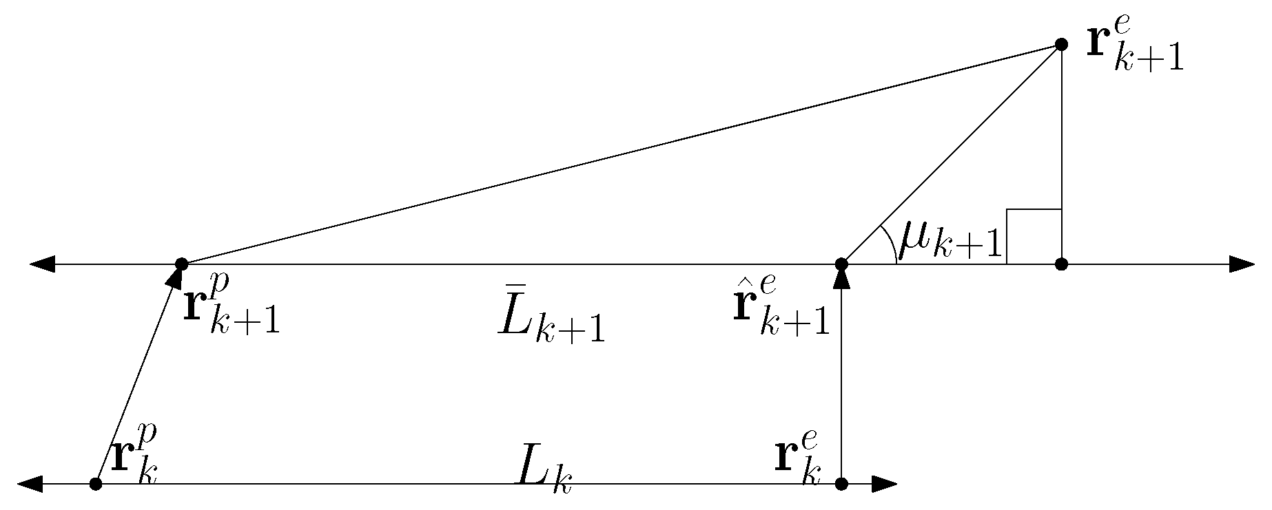
Proof. 

See Figure 3 for an illustration of ${\mu }_{k+1}$. Utilizing the geometry in this figure, we derive

$$\begin{array}{c}\hfill sin(\angle ({\mathbf{r}}_{k+1}^p-{\widehat{\mathbf{r}}}_{k+1}^e,{\mathbf{r}}_{k+1}^p-{\mathbf{r}}_{k+1}^e))=\frac{sin({\mu }_{k+1})\parallel {\mathbf{n}}_{k+1}\parallel }{d_{k+1}}.\end{array}$$

(35)

Since the pursuer at time index k can only access ${\widehat{\mathbf{r}}}_{k+1}^e$ instead of ${\mathbf{r}}_{k+1}^e$, we draw ${\overline{L}}_{k+1}$ intersecting ${\widehat{\mathbf{r}}}_{k+1}^e$ such that ${\overline{L}}_{k+1}$ is parallel to $L_k$. See Figure 3 for an illustration. Utilizing our chasing controller ${\mathbf{u}}_k$, ${\mathbf{r}}_{k+1}^p$ is the heading point on ${\overline{L}}_{k+1}$. Utilizing the same argument as in Theorem 1, we obtain

$$\begin{array}{c}\hfill \angle ({\mathbf{r}}_{k+1}^p-{\widehat{\mathbf{r}}}_{k+1}^e,{\mathbf{r}}_k^p-{\mathbf{r}}_k^e)=0.\end{array}$$

(36)

Utilizing (35) and (36), we derive

$$\begin{array}{c}\hfill sin(\angle ({\mathbf{r}}_k^p-{\mathbf{r}}_k^e,{\mathbf{r}}_{k+1}^p-{\mathbf{r}}_{k+1}^e))=\frac{sin({\mu }_{k+1})\parallel {\mathbf{n}}_{k+1}\parallel }{d_{k+1}}.\end{array}$$

(37)

 ☐

Theorem 3 depicts that in the case where $d_{k+1}$ is too small compared to $sin({\mu }_{k+1})\parallel {\mathbf{n}}_{k+1}\parallel$, $\angle ({\mathbf{r}}_{k+1}^p-{\mathbf{r}}_{k+1}^e,{\mathbf{r}}_k^p-{\mathbf{r}}_k^e)$ is large. In other words, the rotation rate of LOS is large. This implies that the pursuer may leave the motion camouflage state as the distance between the evader and the pursuer is too small.

5. MATLAB Simulation Results

In this section, we demonstrate the effectiveness of our chasing controller utilizing simulations.

$(x(k),y(k))-{\mathbf{r}}_k^e$ represents sensor measurement noise and is a vector with two elements. Each element in this vector has a Gaussian distribution with mean 0 and covariance 0.01. To predict the evader’s location two steps forward in time, we utilize recent $K=5$ measurements.

Initially, the evader is at (0, 5000), and the pursuer is at the origin. $T=2$ s. In addition, the initial speed of the pursuer is 150 m/s. In the terminal phase, $v_k^p$ decreases with respect to k until $v_k^p$ converges to 110 m/s. The pursuer’s maximum acceleration is $a_m$ = 10 m/s${}^2$.

Initially, the pursuer’s heading is ${\mathbf{u}}_0=(1,0)$. In the simulations, we set the maximum turn rate of the pursuer as $q=\pi /6$ radians per second.

MATLAB simulation runs for finite time, at the end of which the distance between the pursuer and the evader is less than 100 m. Recall that the evader’s motion model is presented in (2).

The authors of [8] introduced Frenet-Serret frames [33] to model the movement of an evader.

$$\begin{array}{ccc}\hfill {\mathbf{r}}_{k+1}^e& =& {\mathbf{r}}_k^e+T\ast v_k^e\ast {\mathbf{x}}_k^e\hfill \\ \hfill {\mathbf{x}}_{k+1}^e& =& {\mathbf{x}}_k^e+T\ast v_k^e\ast u_k^e\ast {\mathbf{y}}_k^e\hfill \\ \hfill {\mathbf{y}}_{k+1}^t& =& {\mathbf{y}}_k^e-T\ast v_k^e\ast u_k^e\ast {\mathbf{x}}_k^e,\hfill \end{array}$$

(38)

where $u_k^e$ is the steering (i.e., curvature) control of the evader at time index k, and $v_k^e$ is the speed of the evader at time index k. Recall that ${\mathbf{r}}_k^e$ is the location of the evader at time index k. Moreover, ${\mathbf{x}}_k^e$ is the unit tangent vector to the trajectory of the evader at time index k, and ${\mathbf{y}}_k^e$ is the corresponding unit normal vector at time index k. We utilize (38) to simulate the motion of the evader.

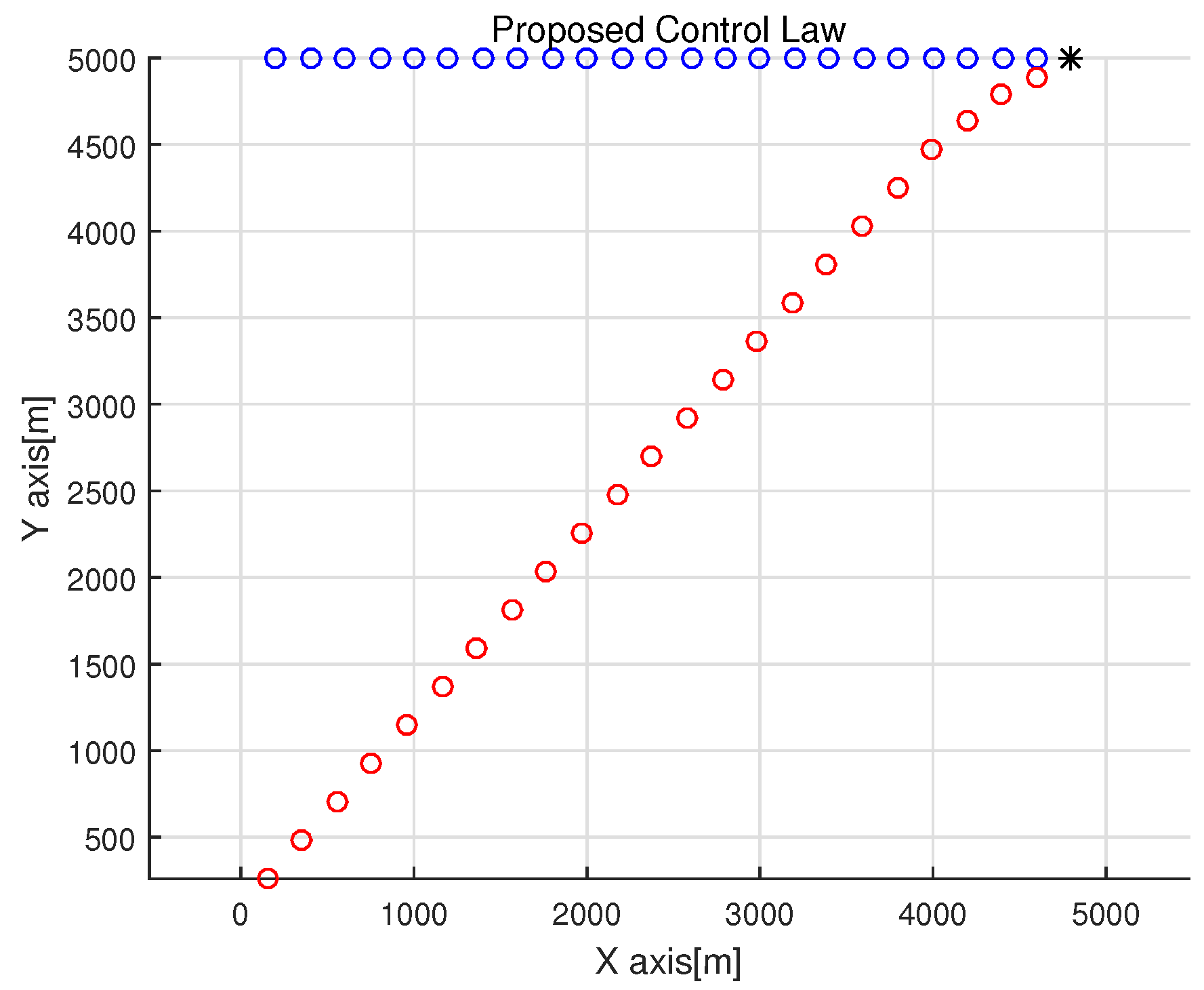
As the first scenario, we set the evader’s speed as $v_k^e=100$ in m/s. In addition, the evader does not maneuver, i.e., $u_k^e=0$. Figure 4 shows pursuer and evader trajectories. In this figure, the pursuer is depicted with red points, and the evader is depicted with blue points. Initially, the pursuer turns towards the evader with the maximum turn rate q. Thereafter, the pursuer converges to the motion camouflage state.

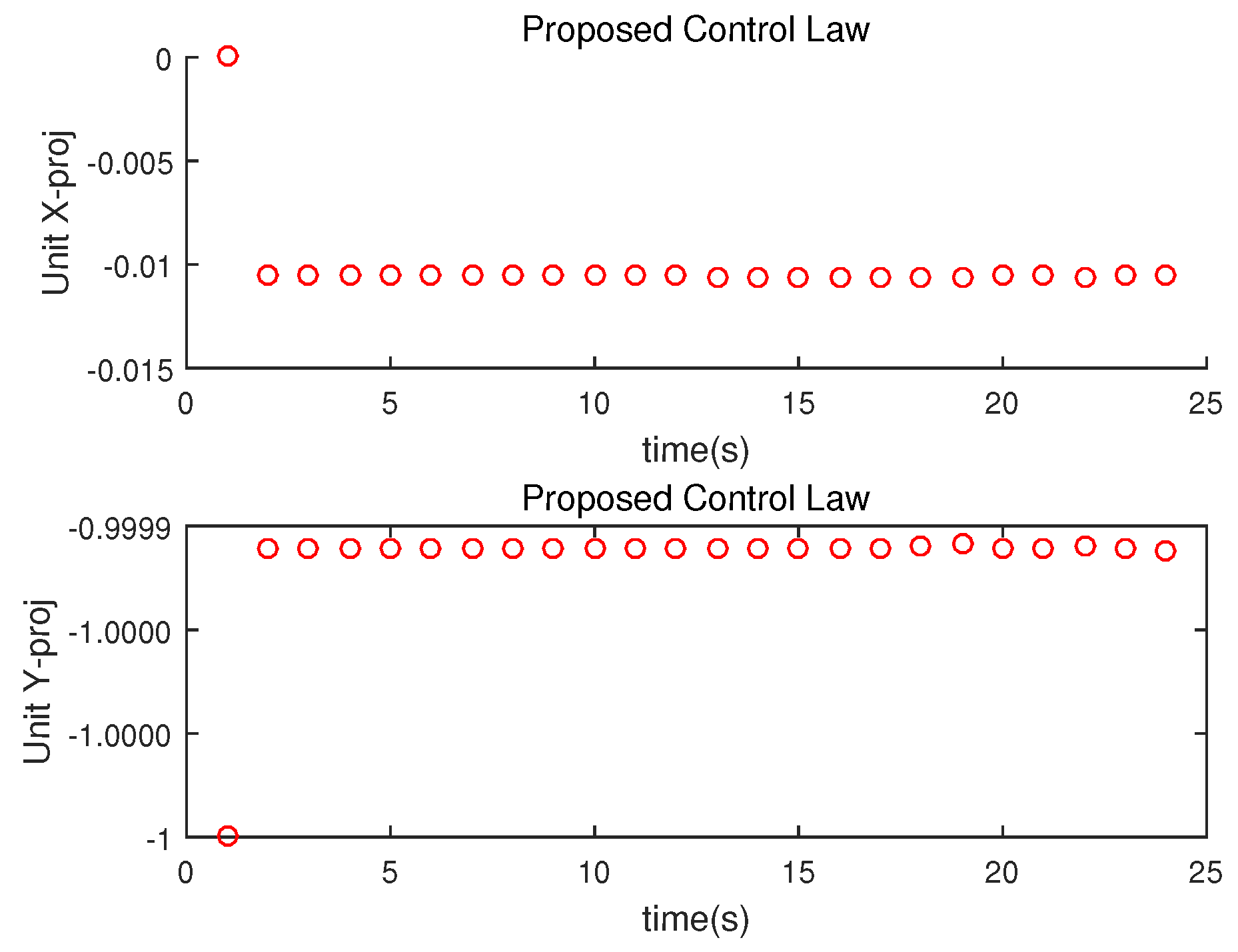
In Figure 5, $\mathbf{l}=\frac{{\mathbf{r}}^e-{\mathbf{r}}^p}{\parallel {\mathbf{r}}^e-{\mathbf{r}}^p\parallel }$ is plotted. $UnitX-proj$ and $UnitY-proj$ indicate the projection of $\mathbf{l}$ on the x-axis and y-axis respectively. The change of these values with respect to time indicates the rotation rate of LOS at every time index. For a pursuit-evasion system in the motion camouflage state, $\mathbf{l}$ converges. Hence, $UnitX-proj$ and $UnitY-proj$ also converge.

Figure 5 depicts that a pursuit-evasion system converges to the motion camouflage state. The chasing controller is designed to converge to the motion camouflage state at time index 0. But, we set $q=\pi /6$ radians per second in the simulation. Due to the constraint on the maximum turn rate, the pursuer cannot converge to the motion camouflage state at time index 0. The pursuer turns with the maximum turn rate until reaching the motion camouflage state. As the pursuer reaches the motion camouflage state, it stays in the state.

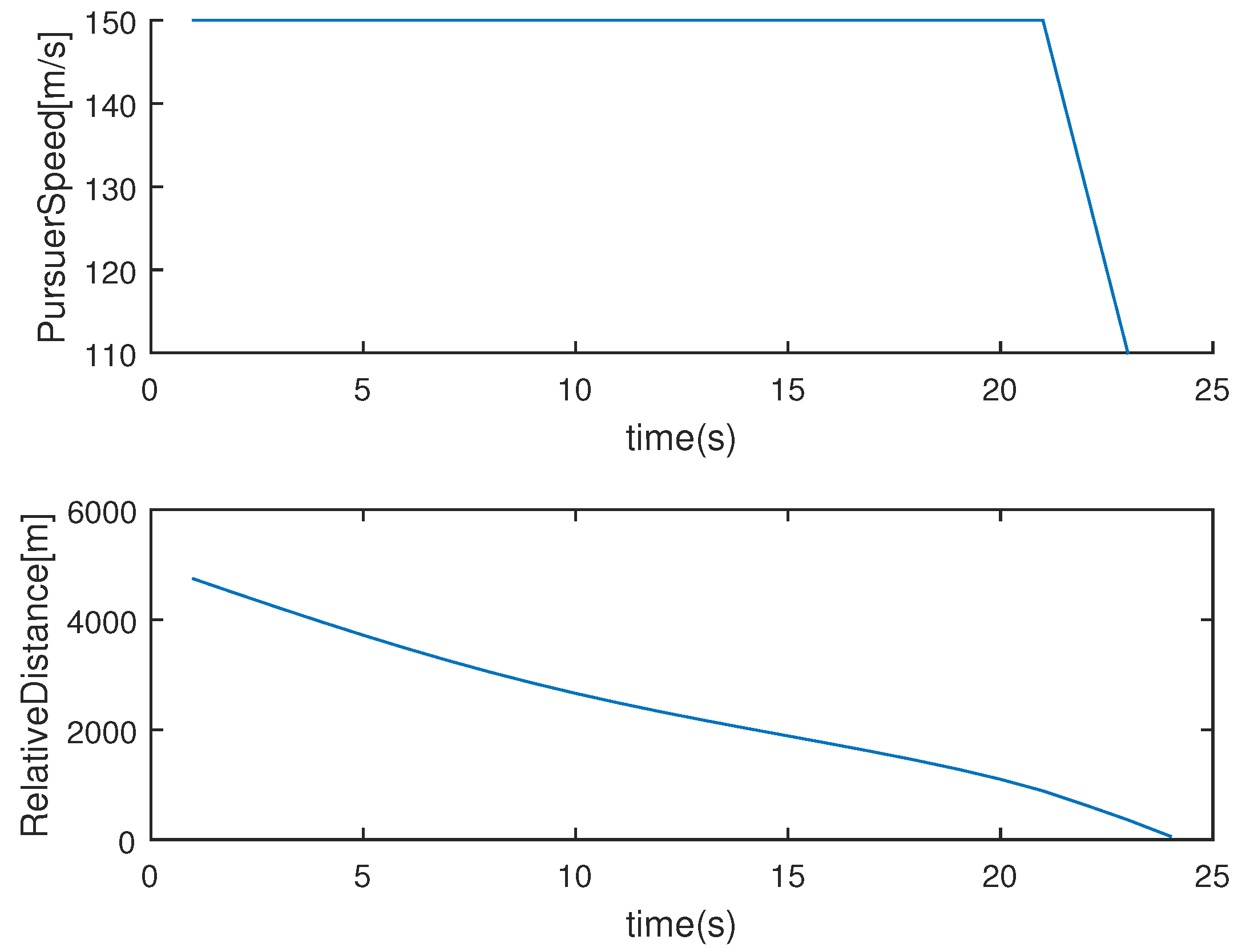
The top figure in Figure 6 depicts the pursuer’s speed with respect to time. See that in the terminal phase, the pursuer adjusts its speed so that it can capture the evader with low speed. Since the relative speed of the evader with respect to the pursuer is low, the probability to the evader is also low. The bottom figure in Figure 6 depicts the distance between the evader and the pursuer with respect to time. Even though the pursuer slows down in the terminal phase, the distance monotonically decreases as time passes.

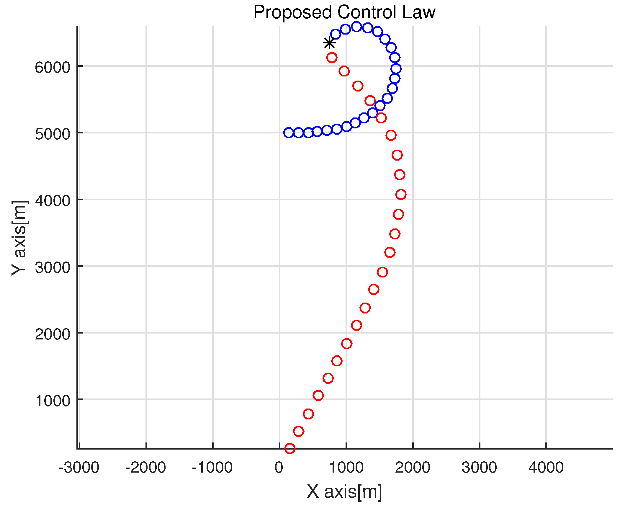
As the second scenario, we set the evader’s speed as $v_k^e$ = 70 + 30 × sin(T × k × 0.01) in m/s. This implies that the evader changes its speed. In addition, the evader maneuvers using $u_k^e$ = 0.005 × sin(T × k/100). Figure 7 shows pursuer and evader trajectories.

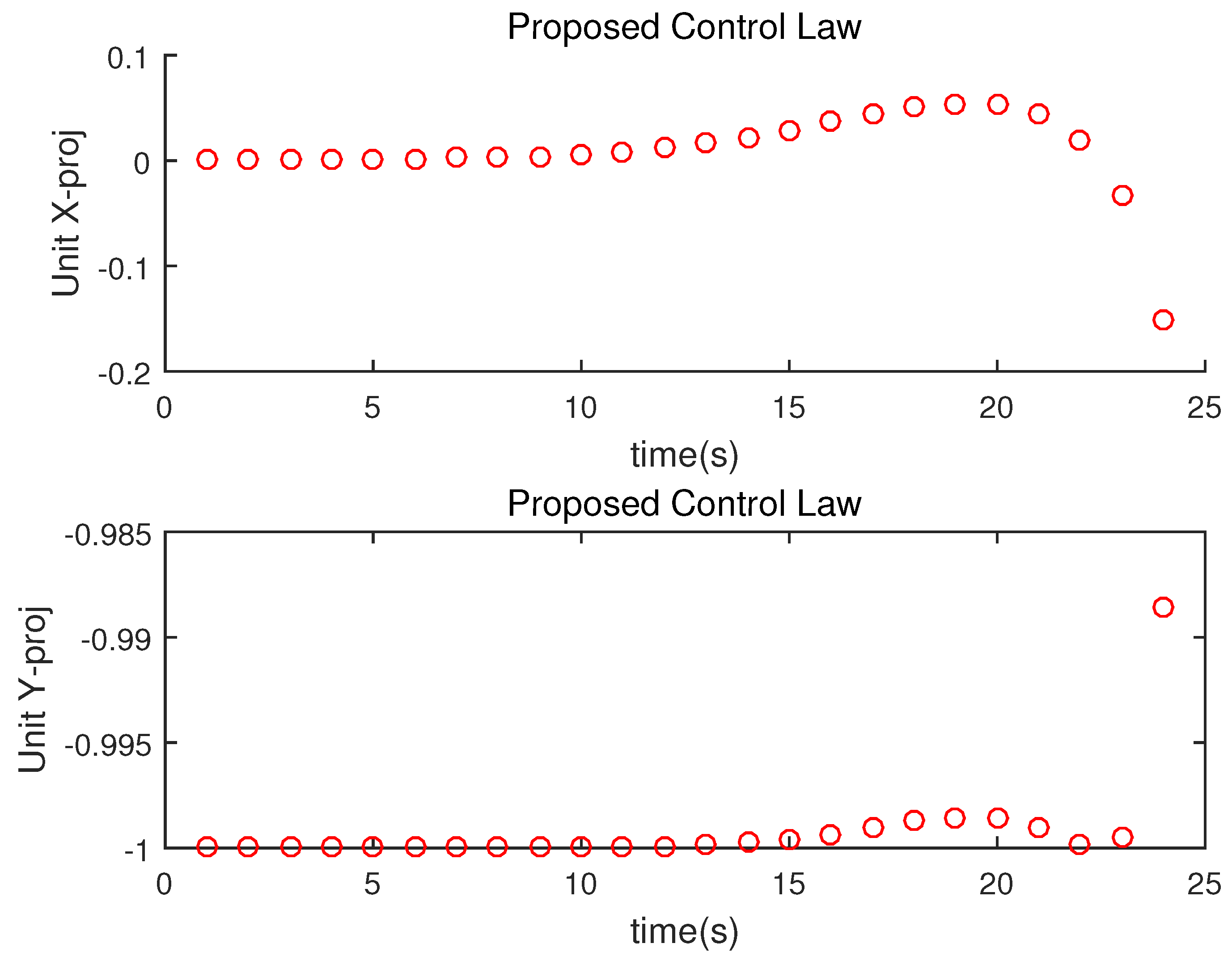
In Figure 8, $\mathbf{l}=\frac{{\mathbf{r}}^e-{\mathbf{r}}^p}{\parallel {\mathbf{r}}^e-{\mathbf{r}}^p\parallel }$ is plotted. $UnitX-proj$ and $UnitY-proj$ indicate the projection of $\mathbf{l}$ on the x-axis and y-axis respectively. In the motion camouflage state, $\mathbf{l}$ converges. Hence, $UnitX-proj$ and $UnitY-proj$ also converge. Figure 8 depicts that a pursuit-evasion system converges to the motion camouflage state. But, the pursuer leaves the motion camouflage state as the distance between the evader and the pursuer is too small. This phenomenon can be explained using Theorem 3.

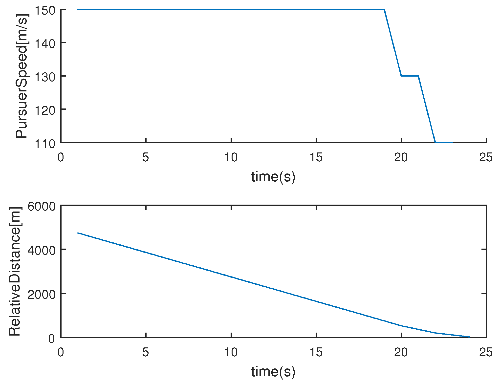
The top figure in Figure 9 depicts the pursuer’s speed with respect to time. See that in the terminal phase, the pursuer adjusts its speed so that it can capture the evader with low speed. The bottom figure in Figure 9 depicts the distance between the evader and the pursuer with respect to time. Even though the pursuer slows down in the terminal phase, the distance monotonically decreases as time passes.

Analysis

We analyze the computational load of our control law. To compute the pursuer’s heading vector ${\mathbf{u}}_k$ at each time index k, it takes 0.03 s. This is negligible compared to the sampling time interval $T=2$ s. Hence, we can argue that latency due to the computational load is negligible.

Next, we run simulations while varying the initial heading angle of the pursuer. We set the evader’s speed as $v_k^e=100$ in m/s. In addition, the evader does not maneuver, i.e., $u_k^e=0$.

We introduce two metrics, $T_f$ and $E_f$. $T_f=k_{f}T$ is the spent time(seconds) to capture the evader. Here, $k_f$ is the time index when the pursuer captures the evader. $E_f={\sum }_{k=1}^{k_f}\parallel v_k^p\angle ({\mathbf{u}}_k,{\mathbf{u}}_{k-1})/T\parallel$. Here, $\angle ({\mathbf{u}}_k,{\mathbf{u}}_{k-1})/T$ is the pursuer’s angular acceleration at time index k. $E_f$ can be regarded as the energy (acceleration sum in m/s${}^2$) required to capture the evader.

The pursuer’s initial location is the origin. We calculate both $T_f$ and $E_f$ while changing the initial heading angle, say $H=atan2([0,1]$×${\mathbf{u}}_0,[1,0]$×${\mathbf{u}}_0$), of the pursuer from 0 to 180 degrees. Here, the initial heading angle is measured counter-clockwise from the x-axis.

Table 1. Results.

H (degrees)	${\mathit{T}}_{\mathit{f}}$ (s)	${\mathit{E}}_{\mathit{f}}$ (m/s${}^2)$
0	47	238
30	49	321
60	49	242
90	49	164
120	49	242
150	49	321
180	51	405

shows $T_f$ and $E_f$ while changing H. See that the evader is captured regardless of the initial heading angle of the pursuer.

6. Conclusions

This paper introduces a chasing controller to capture a high-speed evader with variable velocity. We handle the case where the pursuer moves with a variable speed and the angular acceleration of the pursuer is controllable. In the terminal phase, we slow down the pursuer’s speed, while assuring that the distance between the evader and the pursuer monotonically decreases as time passes. By slowing down the relative speed of the pursuer with respect to the evader, we can reduce the probability of missing the high-speed evader. We demonstrate the performance of our chasing controller utilizing simulations. As our future works, we will verify the performance of our controller using experiments with mobile robots.

In this paper, we handled motion camouflage with respect to a fixed point at infinity. As our future works, we will develop control laws to handle motion camouflage with respect to a fixed point which is not at infinity. Assuming that the evader can readily observe optical flow, but only poorly detect looming, this pursuer’s movement is hardly detected by the evader.