Development of Efficient and Accurate Parallel Computation Algorithm Using Moving Overset Grids on Background Multi-Domains for Complex Two-Phase Flows

Abstract

The goal of this study involves developing an efficient and accurate parallel computation method for two-phase flow problems including complex moving foreign bodies. The proposed parallel computing techniques are based on the moving body-fitted grids’ overset on background multidomains with grid-overlapping at their interface. First, the cavitation flow over the hemispherical head form is investigated using the two-phase flow solver, which is validated by comparing the numerical and experimental results. Subsequently, the parallel computing technique based on the multidomain method that divides the computational domain into several smaller subdomains is proposed to facilitate more efficient numerical simulations. At the interface of the subdomains, the grid-overlapping method is proposed for more accurate simulations. The illustrative computations indicate that the accuracy of the parallel computation combined with the grid-overlapping method on multidomains is identical to that of the serial computation based on a single block, albeit with a significant reduction in the computation time. Finally, the moving overset grid technique is combined with the background multidomain method and applied to simulate the gust flow that is generated by the pitching motions of the twin hydrofoils. The overset grid technique includes the following three sequential steps: hole-cutting, finding donor cells, and bilinear interpolation. The prediction results for the inflow gust generated by oscillating hydrofoils closely follow the measured results.

1. Introduction

Local static pressure in the vicinity of a foreign body in a liquid decreases to the vapor pressure when the object moves fast, and cavities are generated by the phase change from a liquid to gas. The vaporization of liquid due to decreases in the pressure is generally called cavitation. If the pressure increases again, then the cavity explodes and generates high pressure and heat that can damage a foreign body such as a propeller, a pump, and a nozzle. Thus, the parts are designed for operating without cavitation in their normal operating conditions. Conversely, the cavitation phenomena are used to reduce the viscous drag of a submerged vehicle. The viscosity of gas or vapor is lower than that of a liquid, and the frictional drag of the vehicle is reduced by covering the vehicle body with cavitation. The cruise speed of submerged projectiles, such as supercavitating torpedos, is significantly increased using this principle. In order to maximize the advantage, it is necessary to maintain the cavitation shape over the surface of object under complex external environments. Therefore, it is important to experimentally and numerically predict the cavitation shape. Kopriva et al. [1], Lee et al. [2,3], and Karn et al. [4] experimentally investigated the changes in the cavitation shape due to inflow gust. The experiments were conducted in cavitation tunnels. The gust flow was generated using twin hydrofoils that oscillated in a pitching motion. The change in cavitation shape due to inflow gust was examined by varying the amplitudes and frequencies of the oscillating motion of the hydrofoils.

It is extremely helpful to predict a cavitation flow in the design stage of the aforementioned product types with a certain level of accuracy and efficiency. However, it is challenging to numerically simulate the cavitation flow due to relevant physical issues such as a sharp interface between different phases, phase transition phenomena, and a high variation in the speed of sound based on the varying volume fractions of a fluid mixture. In order to capture the interface, various numerical techniques were proposed, including the homogeneous mixture model [5], volume of fluid (VOF) method [6], level set method [7], and smoothed particle hydrodynamics (SPH) [8]. Among the methods, the homogeneous mixture model is frequently used for its wide applicability. Given the assumption of a local equilibrium state of momentum, momentum conservation equations are solved for the homogeneous mixture, although continuity equations are solved for each phase. The proportions of fluid, vapor, or gas in a homogeneous mixture are expressed using a volume fraction.

The phase transition phenomena are modeled using cavitation models that compute the mass transfer rate from a fluid to vapor or vice versa. The model by Merkle et al. [9] is frequently used for its dependence on the proportion of volume fraction and difference between the local and vapor pressure. The term is added to the continuity equation as a source term.

The high variation in the speed of sound is based on the density variation of the fluid mixture and lowers the convergence rate of numerical solutions, because it depends on the lowest speed of sound. In order to solve the problem, the preconditioning method first proposed by Turkel [10] is frequently employed. In the method, the eigenvalues of the flux matrix are modified to reduce the variation in the speed of sound over the entire computational domain [11]. In the preconditioning schemes for steady solutions, the time terms play the role of an iteration index. With respect to unsteady simulations, dual-time stepping methods that use pseudo time in the governing equations are employed [12]. When the residual of the dependent variables is lower than the prescribed criteria in the pseudo time step, the numerical solution simulation proceeds to the next step with respect to physical time. The numerical methods were used in preceding studies, including Kunz et al. [13,14], Lindau et al. [15,16], and Owis et al. [17,18]. The studies developed numerical methods based on dual-time stepping preconditioning techniques to solve incompressible Navier–Stokes equations, and validated the same by comparing their numerical solutions with experimental results [19]. Lindau et al. [20] extended the methods to solve fluid–structure–interaction problems by combining six degree of freedom (DOF) models with the incompressible code and predicting the motion of high speed supercavitating vehicles. Venkateswaran et al. [21,22], Ahuja et al. [23], and Senocak and Shyy [24] added isothermal models to improve the accuracy of a numerical solution for cavitation flow. Kunz et al. [25,26], Lindau et al. [27,28,29], and Owis et al. [30] extended incompressible numerical methods to consider compressibility by solving the compressible Navier–Stokes equations, and attempted to validate the compressible codes by applying the same to various cavitation flows. Kim et al. [31,32] also developed numerical methods to more accurately solve compressible cavitation flows by investigating the effects of turbulence models and viscous flux vectors. Essentially, the numerical method is employed in the current study.

As described above, several numerical techniques were developed to solve physical issues related to the accurate and efficient simulation of cavitation flow. However, the numerical simulation of cavitation flows requires significantly higher computational times due to increases in the number of equations and increases in the variation in the speed of sound when compared with those of single-phase fluid flow. Therefore, several studies have focused on resolving the issue from a different viewpoint that involved adopting parallel computing techniques [33,34]. Domain decomposition methods are generally used to apply the parallel computing techniques for the simulation of cavitation flow, and this divides the complete computational domain into subdomains that are separately treated by each processor. This implies that increases in the number of processors increase the number of subdomains and decrease the computation time, because the size of the domain for each processor decreases. However, the simulation time does not linearly decrease with increases in the number of processors, because the interface boundary between subdomains increases. Specifically, the treatment of the interface boundary between the subdomains is critical for the accuracy and efficiency of the parallel computation.

The interface boundary is categorized into non-overlapping and overlapping methods. In the non-overlapping method, a simple linear interpolation method is applied for information exchange at the interface boundary between subdomains. The method is fast and simple. However, error due to low-order interpolation can adversely affect the accuracy of the numerical result if the interface is subject to a high gradient flow that cannot be avoided when the number of subdomains increases. In the overlapping method, additional interface mesh points that are termed as dummy points are included in each subdomain. At the end of each numerical time integration step over each subdomain, data exchange between subdomains exchange occurs through overlapped points. The dependent variables on the interface boundary of each subdomain are updated using the data on the dummy points.

However, to the best of authors’ knowledge, there has been no systematic analysis on the accuracy of the domain decomposition methods. In the study, the accuracy of the domain decomposition methods is analyzed in combination of the alternating direction implicit (ADI) schemes. Based on the result, the overlapped multidomain method is proposed to be as accurate as the serial single-domain method. In addition, the efficient moving body-fitted overset grid technique is proposed, which can be combined with the background overlapped multidomains method to enable efficient and accurate parallel computations of complex two-phase flow problems involving complex moving foreign bodies. First, cavitation flow over a hemispherical head form is selected as a benchmark problem. The reason for the selection of the problem is two-fold: first, since the problem has been used for the validation of the related numerical methods in a lot of preceding studies, there are a lot of numerical data as well as the experimental data for comparison, and the other is that the final goal of the present development of numerical methods is to investigate the effects of incoming gust on cavitation flows around a high-speed submerged projectile. The current numerical methods based on the preconditioned dual-time stepping compressible Navier-Stokes (NS) equations solvers combined with the cavitation model on serial computation are validated by comparing the prediction results with the measured data. Subsequently, parallel computing techniques combined with the overlapping methods over multiblocks are applied. The validity of the proposed algorithms is confirmed by comparing the numerical results between the parallel computations using the overlapping methods and serial computation. Finally, multidomain methods are combined with the moving overset grid technique to simulate the gust flow generated by twin pitching hydrofoils. The moving body-fitted overset grids are used to model the oscillating hydrofoils, and the multiblocks with overlapping interfaces are used to model the background flow. The validity of the present numerical method is confirmed by comparing the numerical results with measured data.

The governing equations and basic numerical methods are introduced in Section 2. The accuracy of the overlapped multidomain methods in combination with the ADI scheme are analyzed, and the overlapped method, which is as accurate as the corresponding single-domain method, is proposed in Section 3. The numerical results obtained from the serial computation of the cavitation flow over a hemispherical head form are presented and compared with the experimental data, and the parallel computation results obtained from the proposed multidomain methods with the overlapping interfaces are subsequently applied and validated in Section 4. The moving body-fitted overset grid methods consist of three sequential stages, including hole-cutting, finding donor cells, and interpolation, which are described in Section 5. Finally, the numerical results obtained from the application of the present numerical method based on the moving body-fitted overset grids combined with the background overlapped multidomains to the second benchmark problem, including the gust flow that is generated by twin pitching hydrofoils, are presented in terms of their comparison with the measured data in Section 6. The conclusions are detailed in Section 7.

2. Governing Equations and Numerical Methods

In this section, governing equations and numerical methods are described. First, the compressible Reynolds-averaged Navier–Stokes (RANS) equations combined with a homogenous mixture model are presented as the governing equations for cavitation flow. Subsequently, the preconditioning and dual-time stepping methods are briefly described as the numerical methods that are used to solve the governing equations. It should be noted that the numerical methods that are similar to the aforementioned methods were used in studies by Kunz et al. [25,26], Lindau et al. [27,28,29], Owis et al. [18,30], and Kim et al. [31,32].

2.1. Governing Equations

The density-based, unsteady, compressible, two-dimensional, or axisymmetric RANS equations are expressed as follows:

$$\frac{\partial \widehat{q}}{\partial t}+\frac{\partial (\widehat{E}-{\widehat{E}}_v)}{\partial \xi }+\frac{\partial (\widehat{F}-{\widehat{F}}_v)}{\partial \eta }=\widehat{S}$$

(1)

where:

$$\begin{array}{l}\widehat{q}=\frac{1}{J}{\left({\rho }_m{Y}_l,{\rho }_{m}u,{\rho }_{m}v,{\rho }_m{h}_t,{\rho }_m{Y}_v,{\rho }_m{Y}_g\right)}^T\\ \widehat{E}=\frac{1}{J}{\left({\rho }_m{Y}_{l}U,{\rho }_{m}uU+{\xi }_{x}p,{\rho }_{m}vU+{\xi }_{y}p,{\rho }_m{h}_{t}U,{\rho }_m{Y}_{v}U,{\rho }_m{Y}_{g}U\right)}^T\\ \widehat{F}=\frac{1}{J}{\left({\rho }_m{Y}_{l}V,{\rho }_{m}uV+{\eta }_{x}p,{\rho }_{m}vV+{\eta }_{y}p,{\rho }_m{h}_{t}V,{\rho }_m{Y}_{v}V,{\rho }_m{Y}_{g}V\right)}^T\\ \begin{array}{cc}\hfill {\widehat{E}}_v=\frac{1}{J}(0,{\xi }_x{\tau }_{xx}& +{\xi }_y{\tau }_{xy},{\xi }_x{\tau }_{yx}+{\xi }_y{\tau }_{yy},{\xi }_x\left(u{\tau }_{xx}+v{\tau }_{xy}-q_x\right)\hfill \\ & +{\xi }_y\left(u{\tau }_{yx}+v{\tau }_{yy}-q_y\right),0,0{)}^T\hfill \end{array}\\ \begin{array}{cc}\hfill {\widehat{F}}_v=\frac{1}{J}(0,{\eta }_x{\tau }_{xx}& +{\eta }_y{\tau }_{xy},{\eta }_x{\tau }_{yx}+{\eta }_y{\tau }_{yy},{\eta }_x\left(u{\tau }_{xx}+v{\tau }_{xy}-q_x\right)\hfill \\ & +{\eta }_y\left(u{\tau }_{yx}+v{\tau }_{yy}-q_y\right),0,0{)}^T\hfill \end{array}\\ \begin{array}{cc}\hfill \widehat{S}=\frac{1}{J}(({\dot{m}}^{+}+{\dot{m}}^{-})& -c_a{Y}_l{\rho }_{m}v/y,{\rho }_m{g}_x-c_a({\rho }_{m}uv-{\tau }_{xy})/y,{\rho }_m{g}_y\hfill \\ & -c_a({\rho }_m{v}^2-{\tau }_{xy})/y,c_a(u{\tau }_{xy}+v{\tau }_{yy}-{\rho }_m{h}_{t}v-q_y)/y,-({\dot{m}}^{+}+{\dot{m}}^{-})\hfill \\ & -c_a{Y}_v{\rho }_{m}v/y,-c_a{Y}_g{\rho }_{m}v/y){}^T\hfill \end{array}\end{array}$$

(2)

A description of the variables used in Equations (1) and (2) is shown in

Table 1. Nomenclature in Equations (1) and (2).

u, v	Velocity	Y	Mass fraction	τ	Viscous stress
p	Static pressure	ht	Total enthalpy	$\dot{m}$	Mass transfer rate
t	Physical time	ρ	Density	q	Heat flux
U, V	Contravariant Velocity	g	Acceleration of Gravity	ca	1: Axisymmetric flow 0: Planar flow

. With respect to a multiphase flow, the homogeneous mixture model [5] is combined in Equations (1) and (2). The model assumes that the dynamics and thermodynamics of each phase are significantly coupled such that the dynamic and thermodynamic equilibrium states are retained as homogeneous mixtures in the control volume. The multiphase properties are determined by the ratio of each phase, and this is used in the momentum and energy conservation equations, although the continuity equation is applied for each phase. Therefore, the resultant two-dimensional or axisymmetric governing equations consist of three continuity equations for liquid, condensable, and non-condensable gases, two momentum equations, and an energy equation.

2.2. Preconditioning System and Dual-Time Stepping

With respect to the reliable numerical simulation of multiphase flow, preconditioned dual-time stepping methods are employed, and the resultant equations are expressed as follows:

$${\mathsf{\Gamma }}_e\frac{\partial \widehat{Q}}{\partial t}+\mathsf{\Gamma }\frac{\partial \widehat{Q}}{\partial \tau }+\frac{\partial (\widehat{E}-{\widehat{E}}_v)}{\partial \xi }+\frac{\partial (\widehat{F}-{\widehat{F}}_v)}{\partial \eta }=\widehat{S}$$

(3)

where:

$$\begin{array}{c}\widehat{Q}=\frac{1}{J}\left(p,u,v,T,Y_v,Y_g\right)\\ {\Gamma }_e=\frac{\partial \widehat{q}}{\partial \widehat{Q}}\hfill \\ =\left[\begin{array}{cccccc}{Y}_l\frac{\partial {\rho }_m}{\partial p}& 0& 0& Y_l\frac{\partial {\rho }_m}{\partial T}& -{\rho }_m+Y_l\frac{\partial {\rho }_m}{\partial Y_v}& -{\rho }_m+Y_l\frac{\partial {\rho }_m}{\partial Y_g}\\ u\frac{\partial {\rho }_m}{\partial p}& {\rho }_m& 0& u\frac{\partial {\rho }_m}{\partial T}& u\frac{\partial {\rho }_m}{\partial Y_v}& Y_l\frac{\partial {\rho }_m}{\partial Y_g}\\ v\frac{\partial {\rho }_m}{\partial p}& 0& {\rho }_m& v\frac{\partial {\rho }_m}{\partial T}& v\frac{\partial {\rho }_m}{\partial Y_v}& Y_l\frac{\partial {\rho }_m}{\partial Y_g}\\ h_t\frac{\partial {\rho }_m}{\partial p}+{\rho }_m\frac{\partial \mathrm{h}}{\partial p}-1& u{\rho }_m& v{\rho }_m& h_t\frac{\partial {\rho }_m}{\partial T}+{\rho }_m\frac{\partial \mathrm{h}}{\partial T}& h_t\frac{\partial {\rho }_m}{\partial Y_v}+{\rho }_m\frac{\partial \mathrm{h}}{\partial Y_v}& h_t\frac{\partial {\rho }_m}{\partial Y_g}+{\rho }_m\frac{\partial \mathrm{h}}{\partial Y_g}\\ Y_v\frac{\partial {\rho }_m}{\partial p}& 0& 0& Y_v\frac{\partial {\rho }_m}{\partial T}& {\rho }_m+Y_v\frac{\partial {\rho }_m}{\partial Y_v}& Y_v\frac{\partial {\rho }_m}{\partial Y_g}\\ Y_g\frac{\partial {\rho }_m}{\partial p}& 0& 0& Y_g\frac{\partial {\rho }_m}{\partial T}& Y_g\frac{\partial {\rho }_m}{\partial Y_v}& {\rho }_m+Y_g\frac{\partial {\rho }_m}{\partial Y_g}\end{array}\right]\hfill \\ \Gamma =\left[\begin{array}{cccccc}{Y}_l\frac{\partial {\rho }_m^{\prime }}{\partial p}& 0& 0& Y_l\frac{\partial {\rho }_m}{\partial T}& -{\rho }_m+Y_l\frac{\partial {\rho }_m}{\partial Y_v}& -{\rho }_m+Y_l\frac{\partial {\rho }_m}{\partial Y_g}\\ u\frac{\partial {\rho }_m^{\prime }}{\partial p}& {\rho }_m& 0& u\frac{\partial {\rho }_m}{\partial T}& u\frac{\partial {\rho }_m}{\partial Y_v}& Y_l\frac{\partial {\rho }_m}{\partial Y_g}\\ v\frac{\partial {\rho }_m^{\prime }}{\partial p}& 0& {\rho }_m& v\frac{\partial {\rho }_m}{\partial T}& v\frac{\partial {\rho }_m}{\partial Y_v}& Y_l\frac{\partial {\rho }_m}{\partial Y_g}\\ h_t\frac{\partial {\rho }_m^{\prime }}{\partial p}+{\rho }_m\frac{\partial \mathrm{h}}{\partial p}-1& u{\rho }_m& v{\rho }_m& h_t\frac{\partial {\rho }_m}{\partial T}+{\rho }_m\frac{\partial \mathrm{h}}{\partial T}& h_t\frac{\partial {\rho }_m}{\partial Y_v}+{\rho }_m\frac{\partial \mathrm{h}}{\partial Y_v}& h_t\frac{\partial {\rho }_m}{\partial Y_g}+{\rho }_m\frac{\partial \mathrm{h}}{\partial Y_g}\\ Y_v\frac{\partial {\rho }_m^{\prime }}{\partial p}& 0& 0& Y_v\frac{\partial {\rho }_m}{\partial T}& {\rho }_m+Y_v\frac{\partial {\rho }_m}{\partial Y_v}& Y_v\frac{\partial {\rho }_m}{\partial Y_g}\\ Y_g\frac{\partial {\rho }_m^{\prime }}{\partial p}& 0& 0& Y_g\frac{\partial {\rho }_m}{\partial T}& Y_g\frac{\partial {\rho }_m}{\partial Y_v}& {\rho }_m+Y_g\frac{\partial {\rho }_m}{\partial Y_g}\end{array}\right]\hfill \end{array}$$

(4)

Here, Γ_e denotes the flux Jacobian matrix, and Γ denotes the preconditioned matrix. The derivatives of the scaled property are derived as follows:

$$\frac{\partial {\rho }_m^{\prime }}{\partial p}=\frac{\partial {\rho }_m}{\partial p}+\frac{1}{V_p^2}-\frac{1}{c^2}$$

(5)

where V_p denotes the pseudo-acoustic speed that is expressed as follows [35,36]:

$$V_p^2=min\left(max\left(V_a^2,{\beta }_p^2\right),c^2\right)$$

(6)

where $V_a^2$ and ${\beta }_p^2$ denote the cutoff value and local artificial velocity, respectively.

With respect to an unsteady simulation, it is important to select optimum characteristic time scales. However, the pseudo-time term (the second time derivative) is used as the inner or subiteration at each physical time level [12]. In the subiterations, the characteristic time scale is determined with the lowest acoustic time scale in entire computational domain. If the inner iteration simulation converges, then the resultant equations satisfy the full unsteady equations.

2.3. Cavitation Model

The source term ${\dot{m}}^{+}$ and sink term ${\dot{m}}^{-}$ in Equation (2) for the condensation and evaporation rate are respectively expressed as follows [9]:

$$\begin{gathered} {\dot{m}}^{+}=\frac{C_{dest}{\alpha }_l{\rho }_l\min \left(0,p-p_v\right)}{0.5{\rho }_l{U}_{\infty }^2{t}_{\infty }} \\ {\dot{m}}^{-}=\frac{C_{prod}{\alpha }_v{\rho }_v\max \left(0,p-p_v\right)}{0.5{\rho }_l{U}_{\infty }^2{t}_{\infty }} \end{gathered}$$

(7)

where C_dest and C_prod denote empirical constants, and are set as C_dest = 1 and C_prod = 80, respectively, in the present study.

2.4. Turbulence Model

The low-Reynolds number k–ε two-equation turbulence model is used as follows [37]:

$$\begin{gathered} \rho \frac{dk}{dt}=\frac{\partial }{\partial x_j}\left[\left(\mu +\frac{\mu }{{\sigma }_k}\right)\frac{\partial k}{\partial x_j}\right]+P_k-\rho \epsilon +L_k \\ \rho \frac{d\epsilon }{dt}=\frac{\partial }{\partial x_j}\left[\left(\mu +\frac{\mu }{{\sigma }_{\epsilon }}\right)\frac{\partial \epsilon }{\partial x_j}\right]+C_{\epsilon 1}{f}_1{P}_k\frac{\epsilon }{k}-C_{\epsilon 2}{f}_2\rho \frac{{\epsilon }^2}{k}+L_{\epsilon } \end{gathered}$$

(8)

where C_ε1 = 1.44, C_ε2 = 1.92, σ_ε = 1.3, and σ_k = 1.0.

In a cavitation flow, the standard two-equation models are known to overpredict the turbulent eddy viscosity inside the cavity. In order to resolve the problem, a filter-based model is used [38]. The model decreases the viscosity between the turbulence length scale and the filter size, Δ, which is determined by the local grid size. The relevant parameters are defined as follows:

$${\mu }_T=\rho f_{\mu }{C}_{\mu }\frac{k^2}{\epsilon }{f}_{FBM}, f_{FBM}=\min \left(1,\frac{\Delta ·\epsilon }{k^{3/2}}\right)$$

(9)

where C_μ = 0.09.

2.5. Numerical Scheme

The dual-time preconditioned system is numerically solved using the alternating direction implicit (ADI) method [39] in structured grids. The convective flux term is approximated using the monotonic upstream-centered scheme for conservation laws (MUSCL) with third-order accuracy [40]. A second-order backward difference is used to discretize the physical time derivative. A first-order backward difference is used to approximate the pseudo-time derivative. At each physical time step, a pseudo-time iterative procedure is applied with a critical residual of 10⁻⁴.

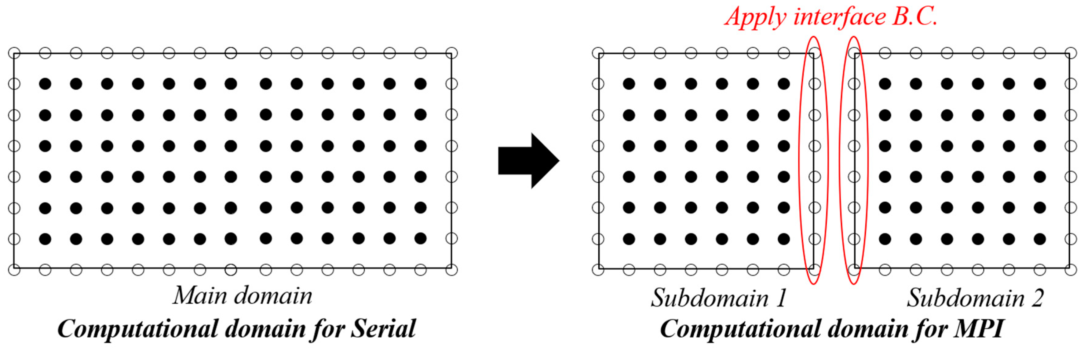
3. Parallel Computation and Grid-Overlapping Interface

In this section, the domain decomposition method combined with the overlapping method is described for the accurate and efficient parallel computation of cavitation flow. First, the domain decomposition strategy is described, and the overlapping methods combined with the ADI scheme are subsequently detailed.

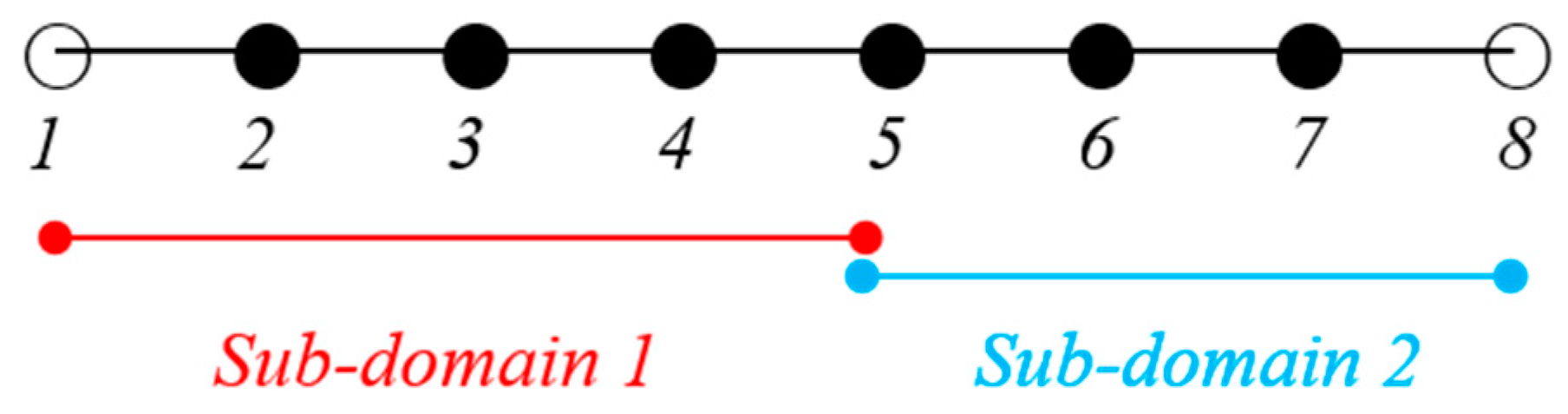
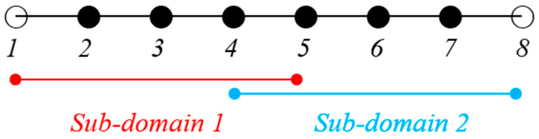
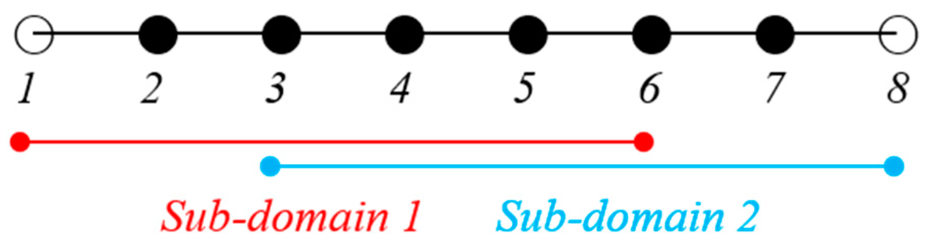
3.1. Domain Decomposition Strategy

As described in the introduction, the numerical simulation for cavitation flow requires expensive computational costs given its physical issues. Parallel computing based on domain decomposition is used to reduce the numerical cost. The domain decomposition methods divide the entire computational domain into smaller domains that are independent of each other and communicate through the interface boundary between neighboring subdomains, and thus, the methods are suitable for parallel computing.

It is important for the overall efficiency of parallel computation to distribute the number of grid points over the subdomains based on the performance of the processor for each subdomain, which is termed load balancing. The most ideal domain decomposition method is that where each processor with an equivalent performance solves the equally distributed subdomain. Subsequently, the performance of numerical simulation is maximized by eliminating the load unbalance that may otherwise occur between the processors. Additionally, the arrangement of subdomains is also critical, and the interface boundary that is parallel to the mean flow is generally preferable because a severe gradient flow can lead to a numerical error during communication between subdomains through the interface boundary. However, with respect to a problem including complex geometries, it is difficult to maintain a lower load on each processor by simultaneously increasing the number of subdomains and the preferable interface boundary lines between the subdomain. In the study, a parallel computation based on the grid-overlapping methods is proposed to resolve the issue by increasing the accuracy of information exchange through the interface boundary between the subdomains.

Figure 1 shows the schematic concept of serial and parallel computations based on single and multidomains, respectively. The single domain consists of interior computational points (black) and boundary points (white), while multi-subdomains consist of interface boundary points (red circles) in addition to the two types of points.

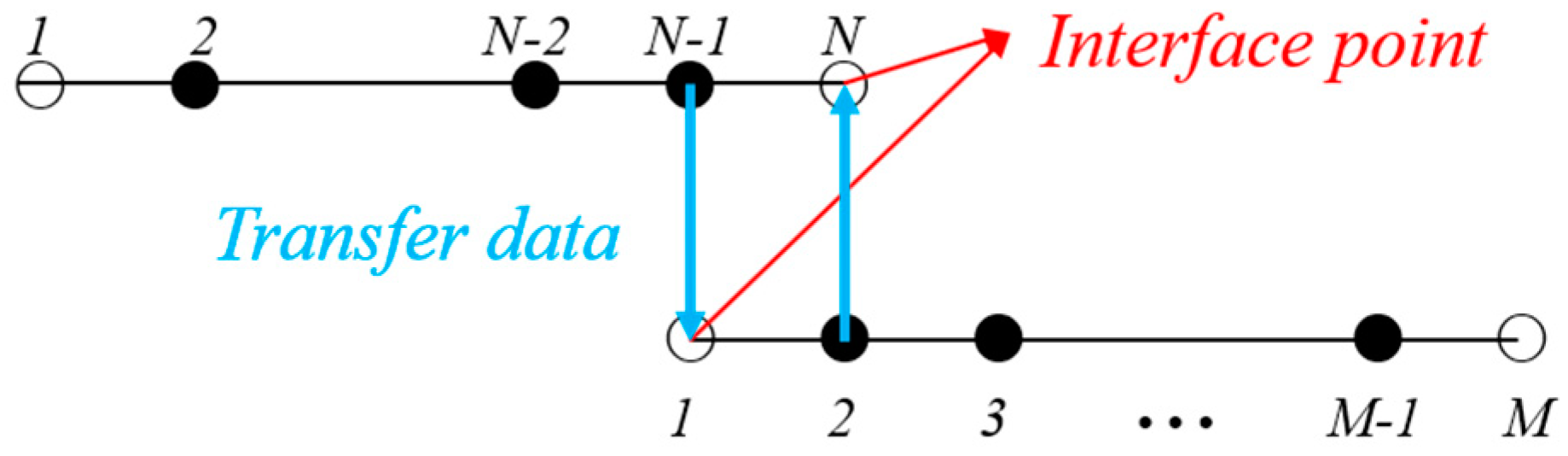
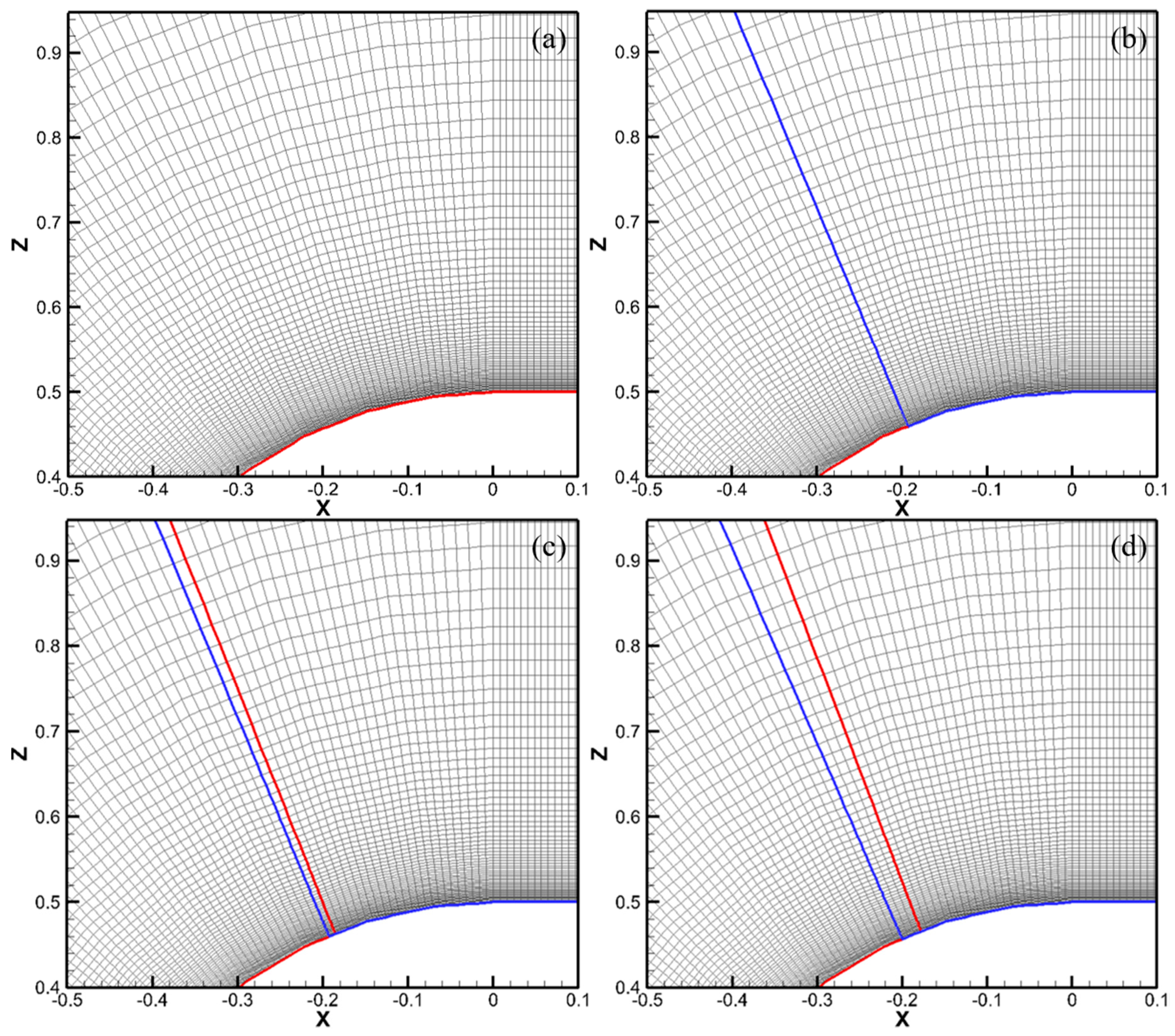
3.2. Grid-Overlapping Interface

As described in the previous section, the governing equation is solved using the ADI method. The method assumes the absence of variations in the values of dependent variables at the boundary points. Thus, the variables on the points in the interface boundary are excluded from the update that is formed using the ADI method, because the interface boundary is also considered as the boundary for each subdomain. Therefore, it is critical to increase the accuracy of information exchange through the interface boundary to improve the overall accuracy of parallel computation. An overlapping method is proposed to achieve the aforementioned purpose.

Figure 2 shows the schematic concept of the overlapping methods. Each subdomain includes dummy points through which the data on the computational points in adjacent subdomains are transferred. The transfer of the data that is computed in adjacent subdomain updates the value on the points in the interface boundary condition with a more reliable value.

For example, the matrix equation of the ADI method with eight points is expressed as follows:

$$\mathrm{S}\Delta \mathrm{Q}=\mathrm{R}$$

(10)

where:

$$\mathrm{S}=\left[\begin{array}{cccccc}{B}_2& C_2& 0& 0& 0& 0\\ A_3& B_3& C_3& 0& 0& 0\\ 0& A_4& B_4& C_4& 0& 0\\ 0& 0& A_5& B_5& C_5& 0\\ 0& 0& 0& A_6& B_6& C_6\\ 0& 0& 0& 0& A_7& B_7\end{array}\right]$$

(11)

With the use of Equation (11), Equation (10) corresponds to a matrix equation formed by applying the ADI method over the single domain. The values of flow variables on points 1 and 8 that are assumed as on the boundary do not exhibit any variation, i.e., ΔQ₁ = ΔQ₈ = 0.

Figure 3 shows the entire domain decomposed into two subdomains without overlapping points, where the first subdomain includes five points from points 1 to 5, and the second subdomain includes four points, from 5 to 8. If the parallel computation based on the domains is performed with a linear interpolation, the matrix S in Equation (11) is modified as follows:

$$S_1=\left[\begin{array}{ccc}{B}_2& C_2& 0\\ A_3& B_3& C_3\\ 0& A_4& B_4\end{array}\right], S_2=\left[\begin{array}{cc}{B}_6& C_6\\ A_7& B_7\end{array}\right]$$

(12)

In the ADI method, variation in the points of boundary condition in each subdomain is absent. The equation omits C₄, A₅, B₅, C₅, and A₆, which exist in Equation (11). This implies that it is not possible to obtain the value on point 5 from the solution of Equation (12). The value on point 5 is typically updated using the linear interpolation of the values on the neighboring points, and this is definitely different from that in Equation (11). The overlapped subdomains are employed to reduce the difference.

Figure 4 shows the overlapped domains with two points that correspond to the minimum in an overlapping method. If the ADI method is applied in the configuration, and Equation (11) subsequently changes as follows:

$$S_1=\left[\begin{array}{ccc}{B}_2& C_2& 0\\ A_3& B_3& C_3\\ 0& A_4& B_4\end{array}\right], S_2=\left[\begin{array}{ccc}{B}_5& C_5& 0\\ A_6& B_6& C_6\\ 0& A_7& B_7\end{array}\right]$$

(13)

In the method, the value on points 4 and 5 is computed by solving Equation (12). However, a difference exists between equations (11) and (13) wherein C₄ and A₅ are missing in Equation (13) when compared with Equation (11). The effect of the difference is negligible with respect to a simulation for a problem with simple geometry or a small number of grids. However, the four-point overlapped method should at least be used to ensure that the numerical solution of parallel simulation is identical to that of the single domain.

As shown in Figure 5, the four-point overlapped method where the numerical solution on the entire grid points is obtained as follows:

$$S_1=\left[\begin{array}{cccc}{B}_2& C_2& 0& 0\\ A_3& B_3& C_3& 0\\ 0& A_4& B_4& C_4\\ 0& 0& A_5& B_5\end{array}\right], S_2=\left[\begin{array}{cccc}{B}_4& C_4& 0& 0\\ A_5& B_5& C_5& 0\\ 0& A_6& B_6& C_6\\ 0& 0& A_7& B_7\end{array}\right]$$

(14)

The values of variables on points 5 and 6 in Subdomain 1 and points 3 and 4 (Subdomain 2) are obtained from its neighboring subdomain. The values are transferred via the interface boundary to the neighboring domain. Therefore, the method provides numerical solutions that are equivalent to that of a single domain, albeit at a lower numerical cost. In the following section, the overlapped methods and serial numerical method are applied to benchmark problems to highlight the accuracy and efficiency of the numerical solutions that are obtained in the present method.

4. Cavitation Flow over the Hemispherical Head Form

In this section, the cavitation flow over hemispherical head form is numerically investigated using serial and parallel computations. The validity of numerical solutions is confirmed by comparing the same with the data measured by Rouse et al. [19]. Additionally, the accuracy of the numerical solution obtained from the parallel computations based on the overlapped methods is confirmed by comparing it with that of the serial computation. The efficiency of parallel computations is highlighted by comparing the computation time with respect to the number of processors that are employed in the computations.

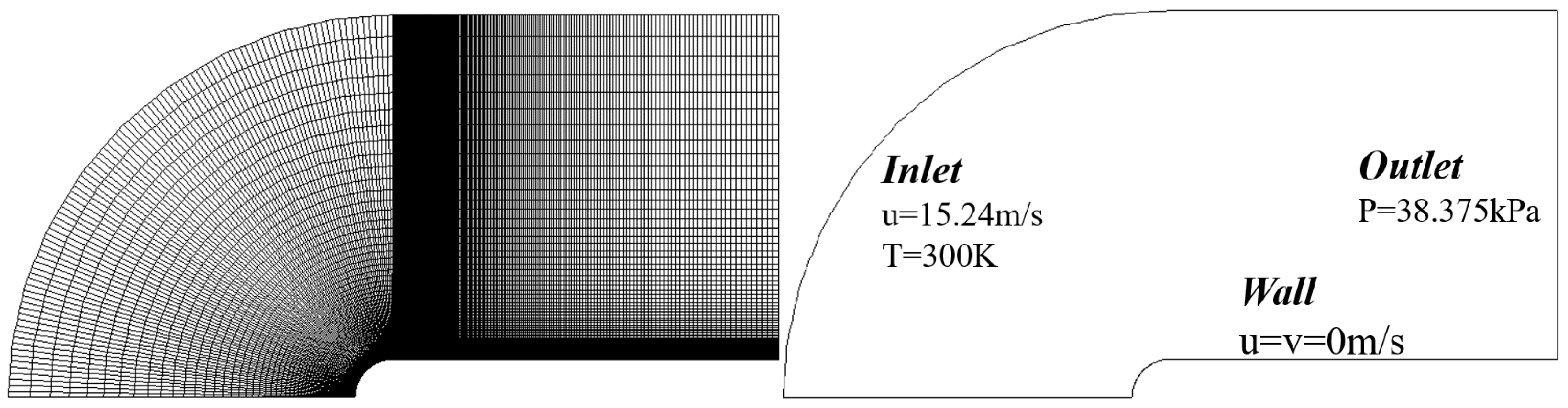
4.1. Computational Domain

Figure 6 shows the entire computational domain and the applied boundary conditions. The number of grids that is used in the serial computation correspond to 300 × 100. The minimum of the Δy at the wall is set as 0.001D. The flow condition is selected based on that in the study by Lindau et al. [28]. The Reynolds number is $1.4\times {10}^5$, the inlet temperature is 300 K, the free stream velocity is u = 15.24 m/s, and the static pressure is 38.375 kPa. In the aforementioned condition, the cavitation number corresponds to σ = 0.3. The no-slip boundary condition is applied on the wall surface. At the inlet boundary, the free stream velocity and temperature are specified with the exception of the static pressure. The static pressure is specified at the outlet boundary. The other parameters on the boundaries are determined by an extrapolation inside the computational domain.

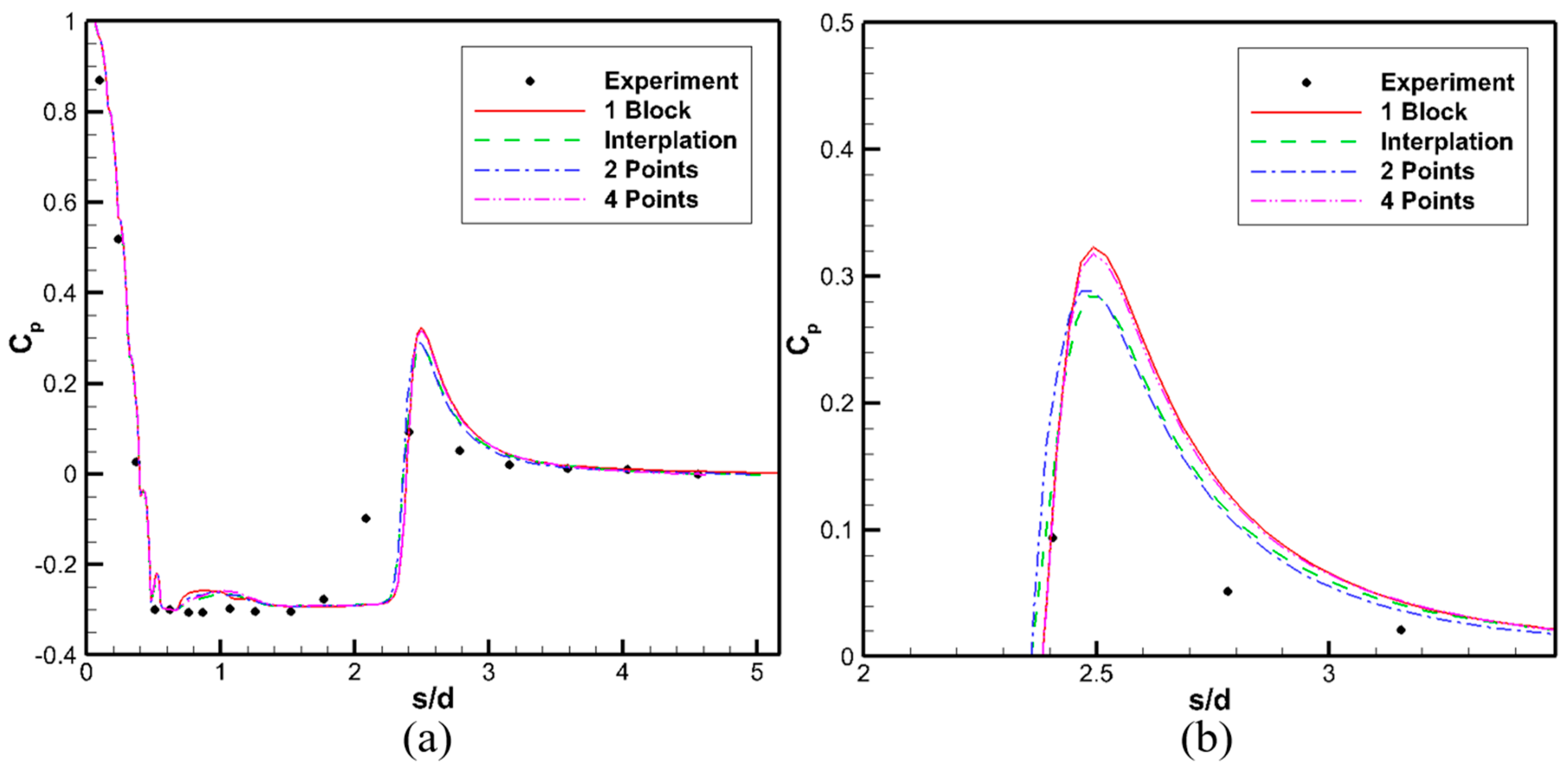
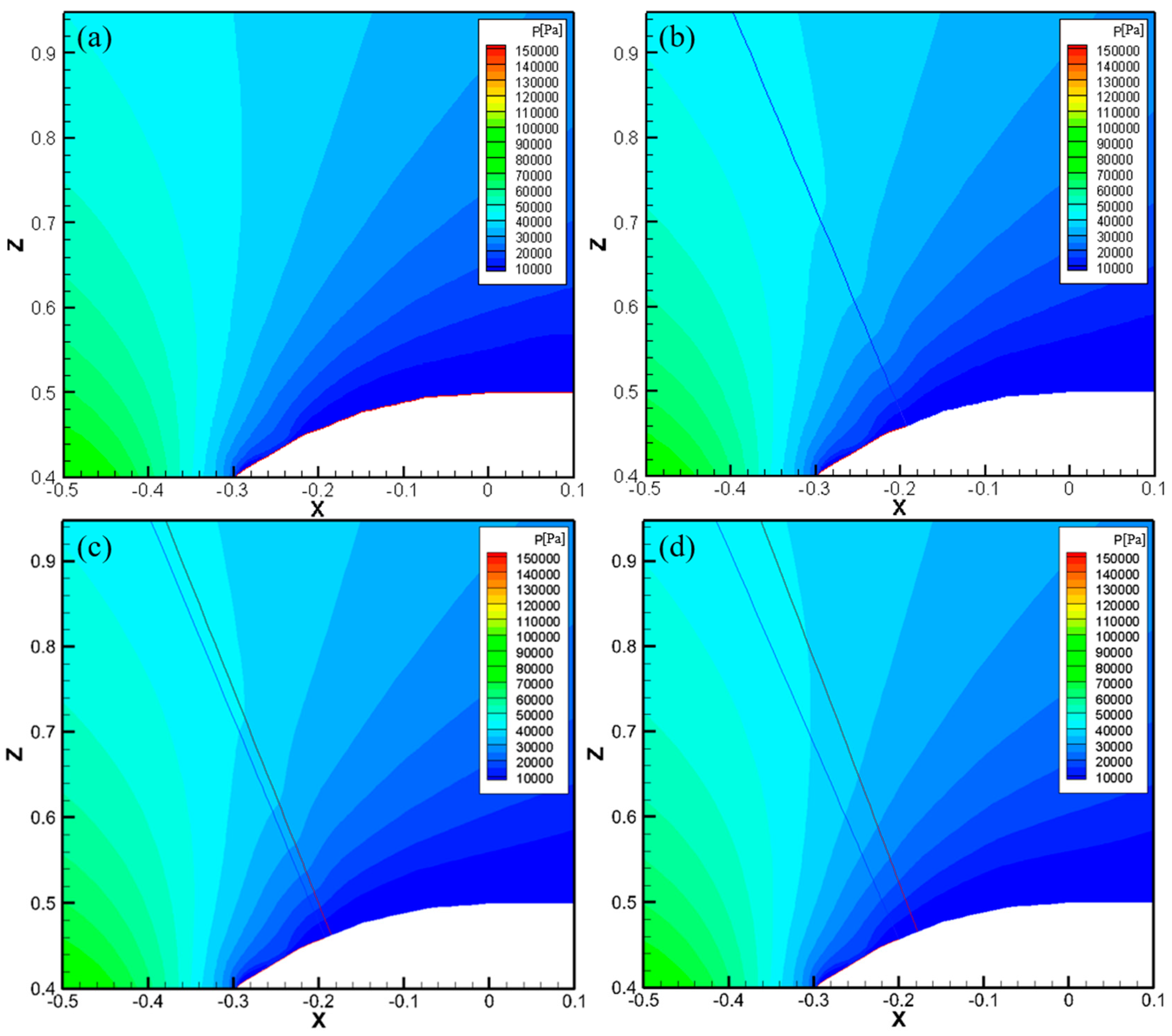
4.2. Interface Boundary Condition

As described in the previous section, interface boundary conditions are required for parallel computations based on multidomain methods, and are critical in terms of the overall accuracy of parallel computations. The types of interface boundary conditions depend on the associated multidomain methods, namely the number of overlapped grid points. Three types of interface boundary conditions, including linear interpolation, two-point overlapped methods, and four-point overlapped methods, are used. Figure 7 shows a magnified view of the grids that were used for the serial and parallel computations. In Figure 7a, the computation domain consists of a single domain used for the serial computation. The results obtained from the serial computation based on the single domain are used as the reference results by which the accuracy and efficiency of the parallel computations are assessed. The validity of the serial computation is confirmed by comparing its results with the measured data. In the other parallel computations, the computational domain consists of multi-subdomains.

Figure 8 shows the distribution of the cavitation flow around the body in terms of the water volume fraction where AL = 1 and AL = 0 denote pure water and vapor, respectively. The overall distributions of cavitation in all of the cases are similar to each other, which confirms the validity of the parallel computations. However, the pressure distributions on the body are compared with the measured data to examine the effects of the interface boundary conditions in further detail.

Figure 9 compares the distributions of the predicted mean pressure coefficients along the body surface. The data measured by Rouse et al. [19] is also provided to confirm the validity of the numerical results. Generally, good agreements are observed between the numerical and experimental results, although there are not enough measured points around the peak for stricter validation. However, the numerical predictions by Owis et al. [17,30] showed results similar to the present ones: the peak value is located more downstream in comparison to the experimental result.

However, all of the numerical results slightly overpredicted the cavity length when compared with the experimental results. The pressure in the cavity is lower than that of the surrounding fluid such that flow is induced inside the cavity, and this causes a re-entrance jet. The cavity length depends on the re-entrance flow, and this implies that the cavity length exhibits high unsteadiness and varies relative to the re-entrance jet phenomena. In all of the numerical simulations, the re-entrance flow occurs at the end of the cavity. The unsteadiness potentially leads to the observed difference between the numerical and the experimental results.

As shown Figure 9, the mean pressure coefficient obtained from the numerical result based on the four-point overlapped method closely follows that of a single domain. The other numerical results obtained from parallel simulations based on the linear interpolation and two-point overlapped grids are slightly lower than those in the single domain. This is due to the difference in the interface boundary conditions that are associated with the number of overlapped points in the parallel simulations. The difference does not appear to be critical to the overall computational accuracy of the simple problem. However, it is not possible to infer the same for problems involving complex geometry. Therefore, as noted in the previous section, the four-point overlapped method is proposed to resolve the issue.

Figure 10 shows the pressure distribution around the interface boundary to highlight the accuracy of the four-point overlapped method. With the exception of the case of the single block and four-point overlapped methods, an abrupt change in the slope of pressure contours is observed across the grid interface line between the subgrids. The discontinuity leads to an observed difference in the mean pressure coefficients, as shown in Figure 9. Overall, the four-points overlapped method for the interface boundary in the parallel computation in combination with the multi-subgrid method provides numerical results with an accuracy that is equal to that of the serial computation at a lower numerical time value. In all of the subsequent parallel numerical simulations, the four-point overlapped method is used to illustrate its efficiency.

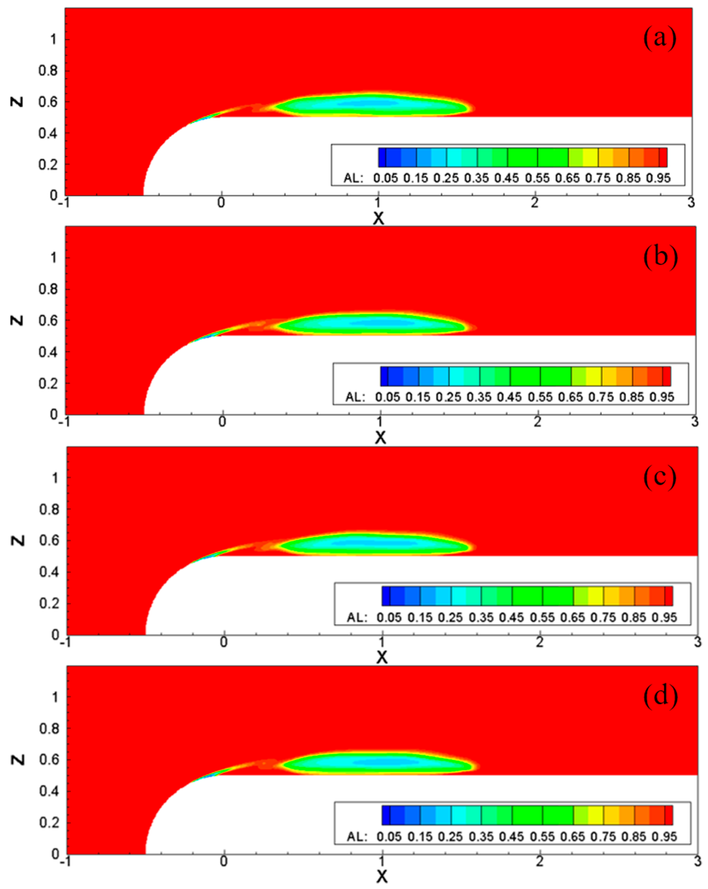
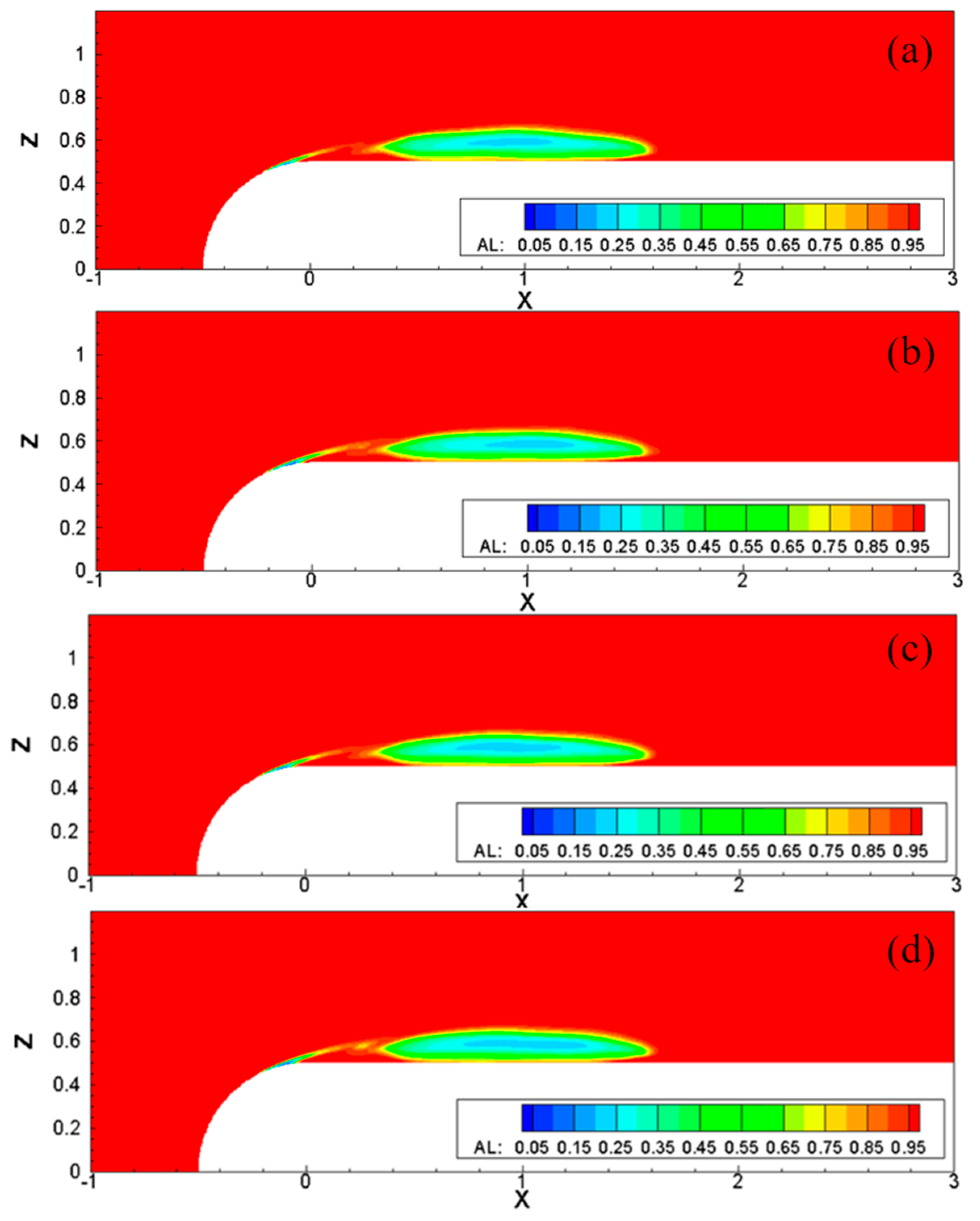
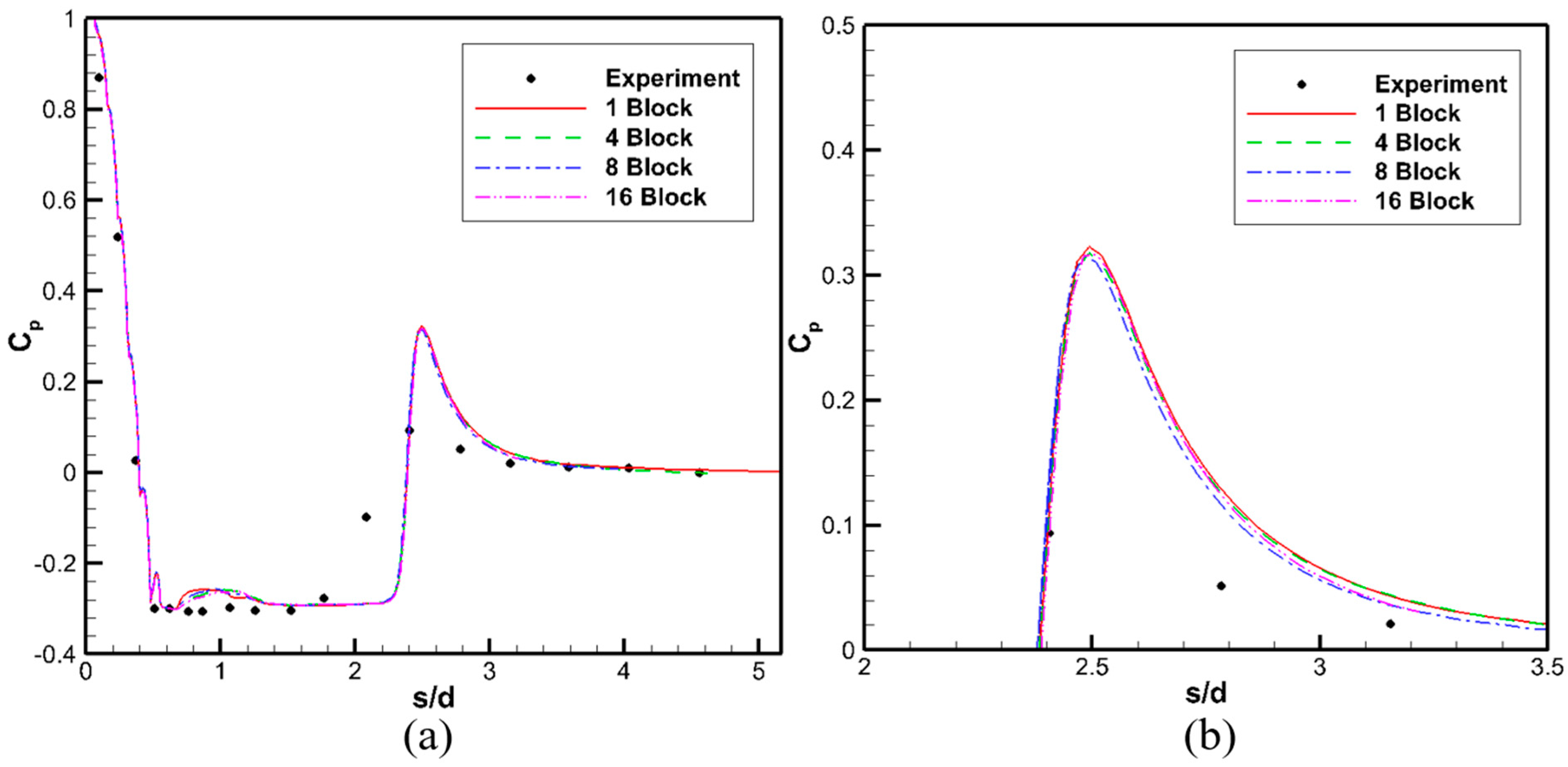
4.3. Number of Subgrid Blocks (or Processors)

In the parallel computations, it is generally expected that the computation time decreases when the number of sub-blocks (or processors) increases. However, the reduction in the computation time does not exhibit a linear decrease. In order to confirm the computing time by varying the number of sub-blocks, computation domains consisting of one, four, eight, and 16 blocks are considered. Figure 11 shows the computation domains. In all of the cases, the four-point overlapped method is used for the interface boundary condition. The other flow and boundary conditions are identical to those in the previous simulations.

Figure 12 shows the distribution of cavitation flow in terms of the water volume fraction for each case. The fact that the overall cavitation distribution exhibits similar pattern indicates that the number of blocks does not significantly affect the accuracy of the numerical solutions.

Figure 13 shows the distribution of the mean pressure coefficient that is obtained from each case in conjunction with the measured data. The results indicate excellent agreement between the serial and parallel computations, although the difference slightly increases when the number of sub-blocks increases.

Figure 14 shows the variation in the numerical costs in terms of the speedup that is defined as T₁/T_n where T denotes the time required to complete the computation, and the subscript denotes the number of processors (or sub-blocks) that are used. As expected, an increase in the number of processors further reduces the computation time. In the simulation, the use of 16 processors reduces the computation time by 12 times. However, it does not decrease linearly, because each subdomain includes overlapped points that imply that the number of total grid increases with increases in the number of sub-blocks. However, the results indicate that the parallel computation based on the multiblock methods in combination with the four-point overlapped grids provides a numerical solution with an accuracy identical to that of the serial computation, albeit at a lower numerical cost.

5. Moving Overset Grid Method

The algorithm of moving chimera grid methods consists of the following three sequential steps: hole-cutting, finding donor cells, and bilinear interpolation [33,41,42,43,44,45]. The steps are described in detail below.

5.1. Hole Cutting

The moving chimera grid method includes a minimum of two grid domains. The domains are classified into two types, namely a background grid and a body-fitted (moving) grid. In the background grid, hole points exist on which the calculation is not necessary, because they belong to the body-fitted grid domains. In order to find the points, the dot product is used as a criterion as follows:

$$\mathrm{Hole} \mathrm{point} \mathrm{if} \overrightarrow{sp}·\overrightarrow{n_s}<0$$

(15)

Figure 15 shows the schematic view of determining the hole points. At the hole points, the variables from the governing equations are set to zero. The points close to the hole points are classified as interpolation points.

5.2. Donor Cell

It is important to determine donor cells that contain target interpolation points. Graham’s scan method [46] is used in the study, although there are several extant methods to identify donor cells. The method uses the cross-product sign. As shown in Figure 16, the values of the cross product between the vectors defined along the side edge of the cell (green-colored vector) and the vector formed between the vertex of the cell and the interpolation points (yellow-colored vector) are always positive, because the product order is in a counterclockwise direction as follows (in a two-dimensional space):

$$\overrightarrow{f_1{f}_2}\times \overrightarrow{f_{1}P}\ge 0, \overrightarrow{f_2{f}_3}\times \overrightarrow{f_{2}P}\ge 0, \overrightarrow{f_3{f}_4}\times \overrightarrow{f_{3}P}\ge 0, \overrightarrow{f_4{f}_1}\times \overrightarrow{f_{4}P}\ge 0$$

(16)

The values are negative when the product order is reversed in a clockwise direction. The donor cell for interpolation is identified using the method.

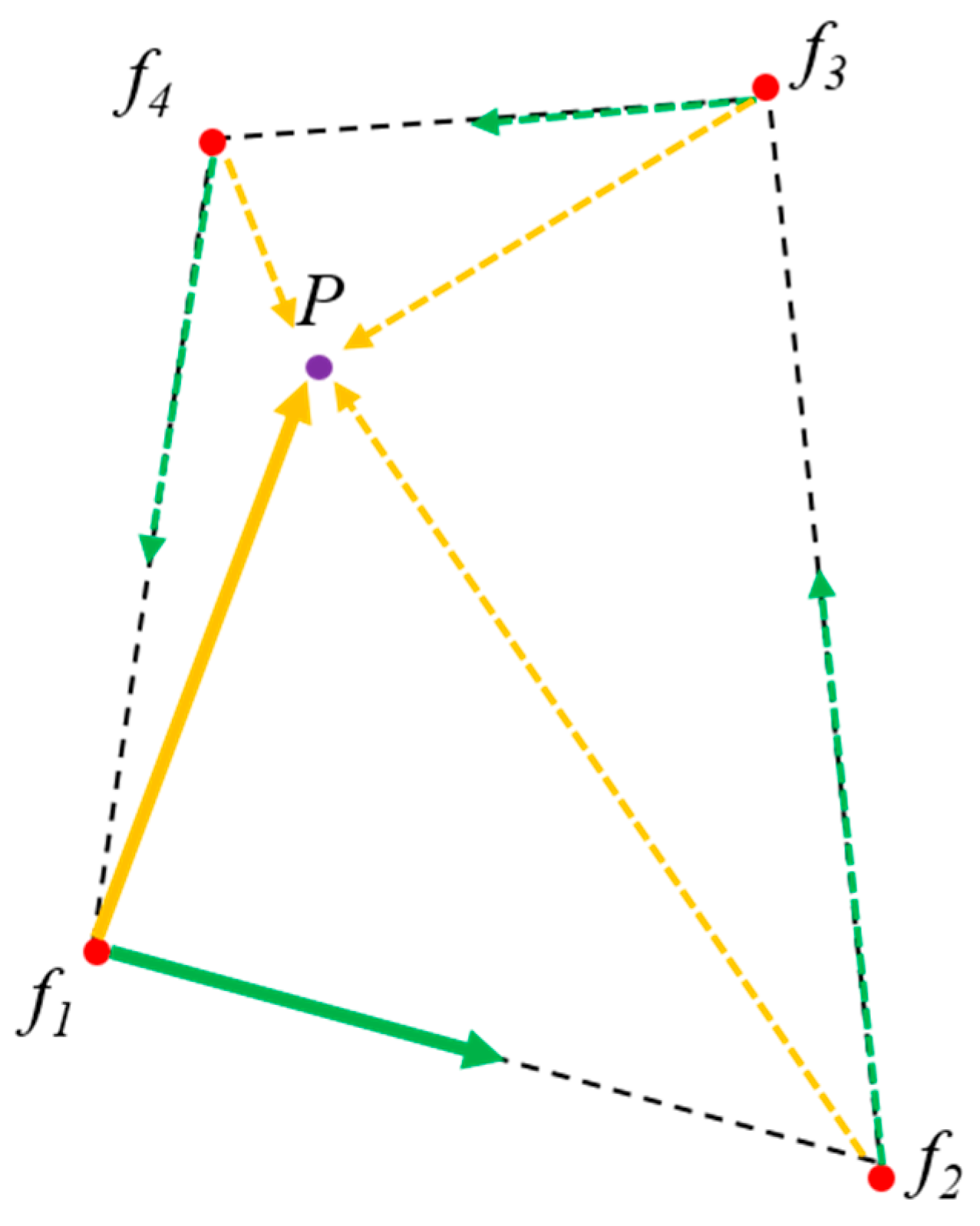
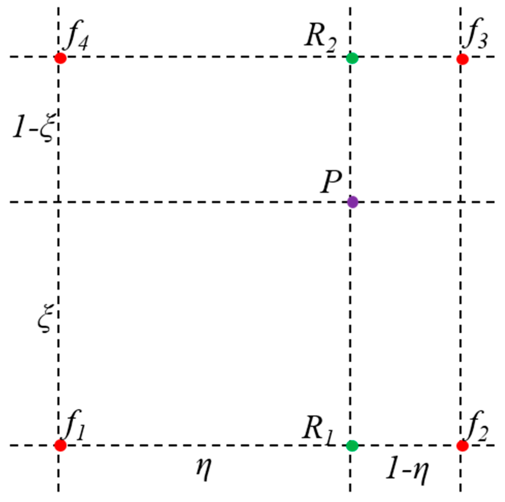
5.3. Bilinear Interpolation

With respect to various interpolation methods, bilinear interpolation [47] is used for its simplicity as follows:

$$P=\left(1-\xi \right)\left(1-\eta \right)f_1+\xi \left(1-\eta \right)f_2+\left(1-\xi \right)\eta f_3+\xi \eta f_4$$

(17)

The unknown values of ξ and η correspond to the rate of distance and are determined from the coordinates, as shown in Figure 17. The values of the physical variables at the point P are determined using Equation (17). The interpolation method is applied to the interpolation points in the background grid domain and the boundary points in the body-fitted grid domain.

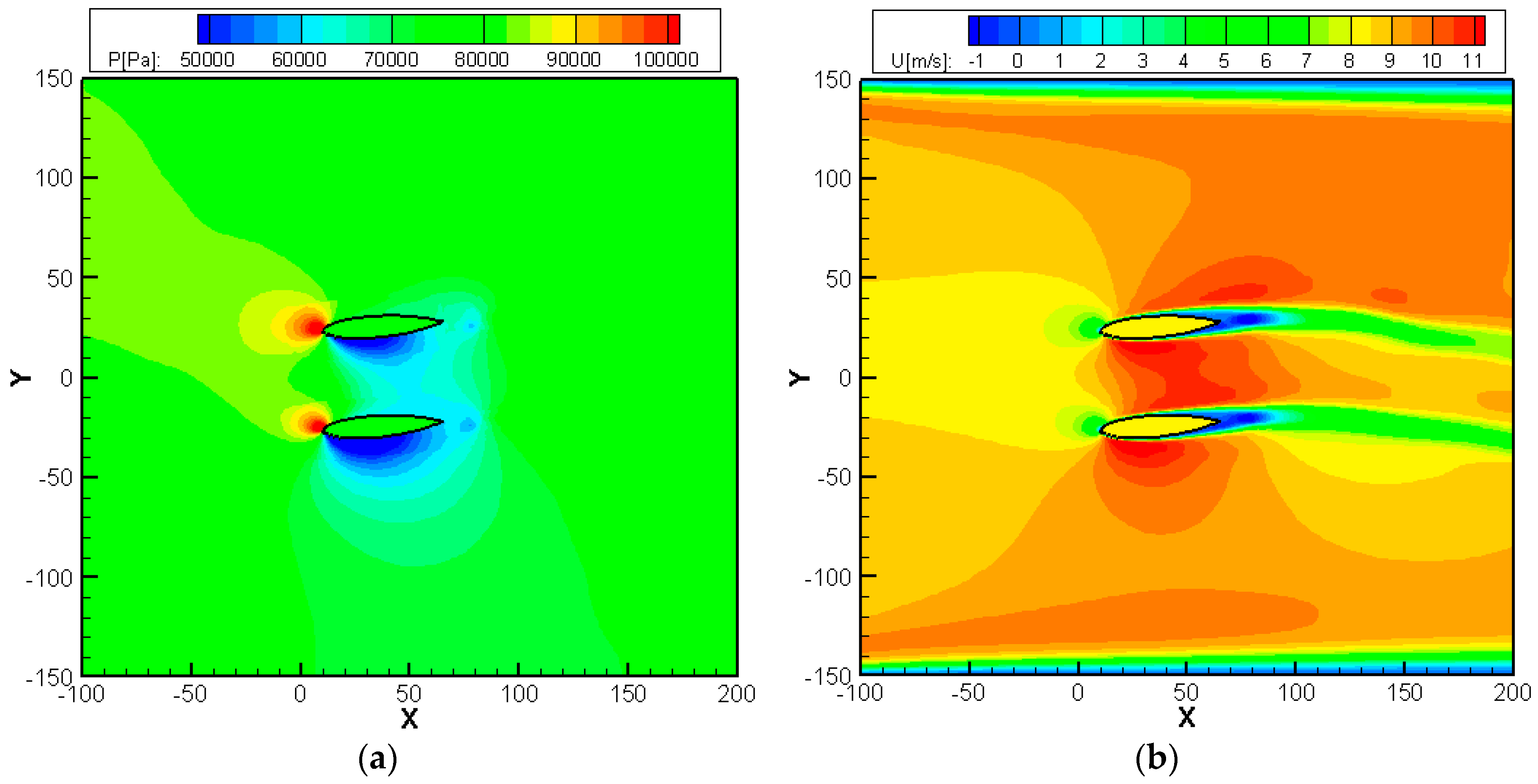
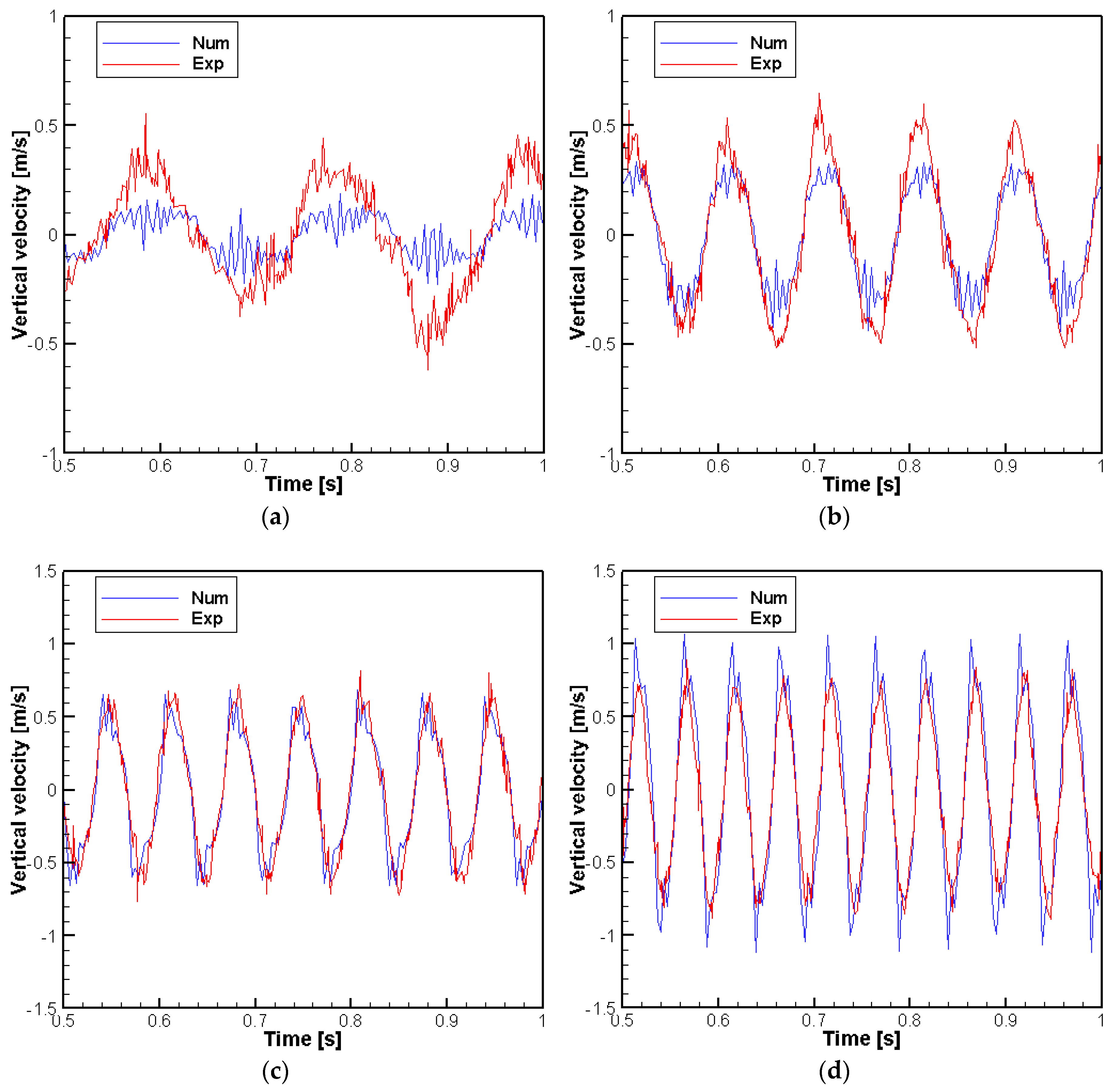
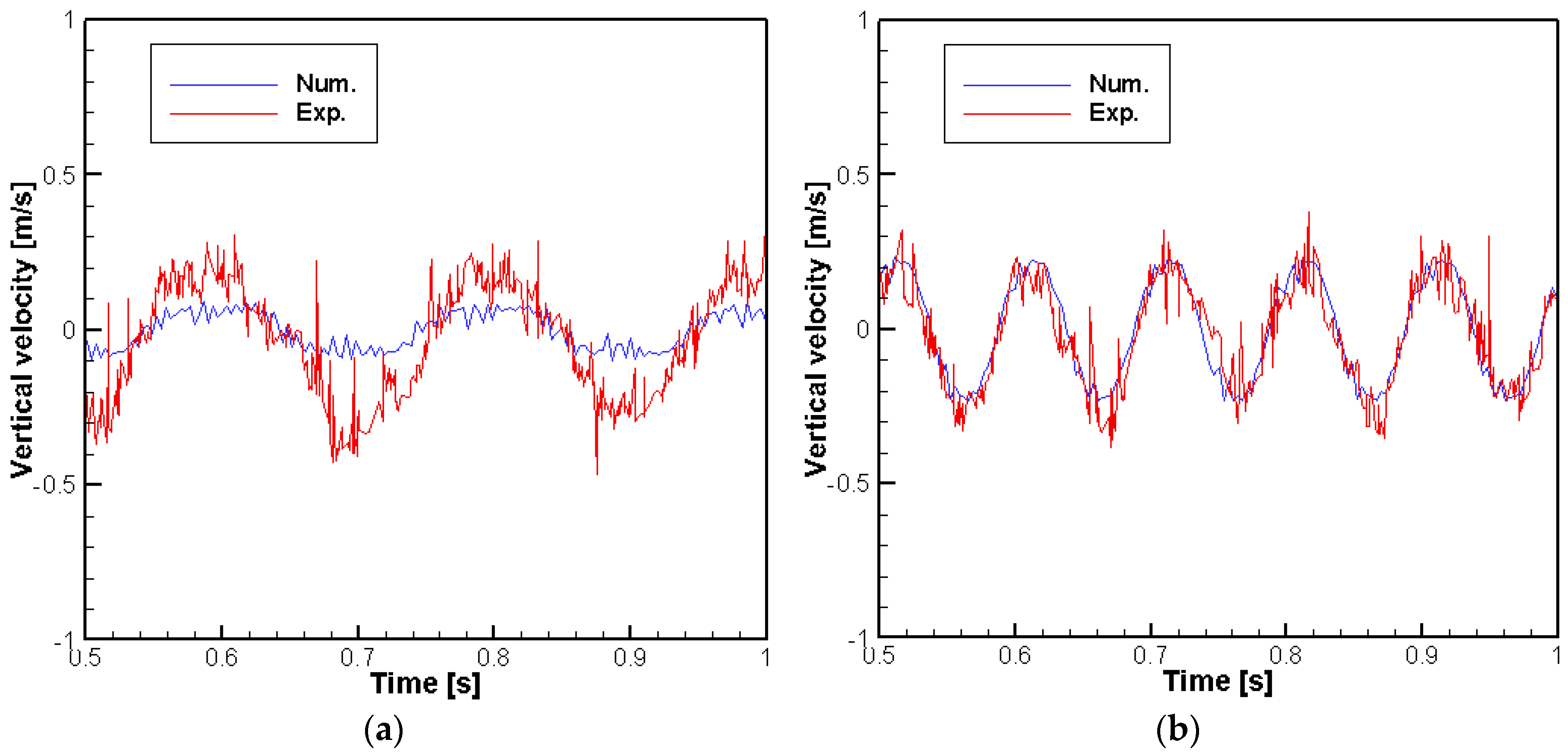
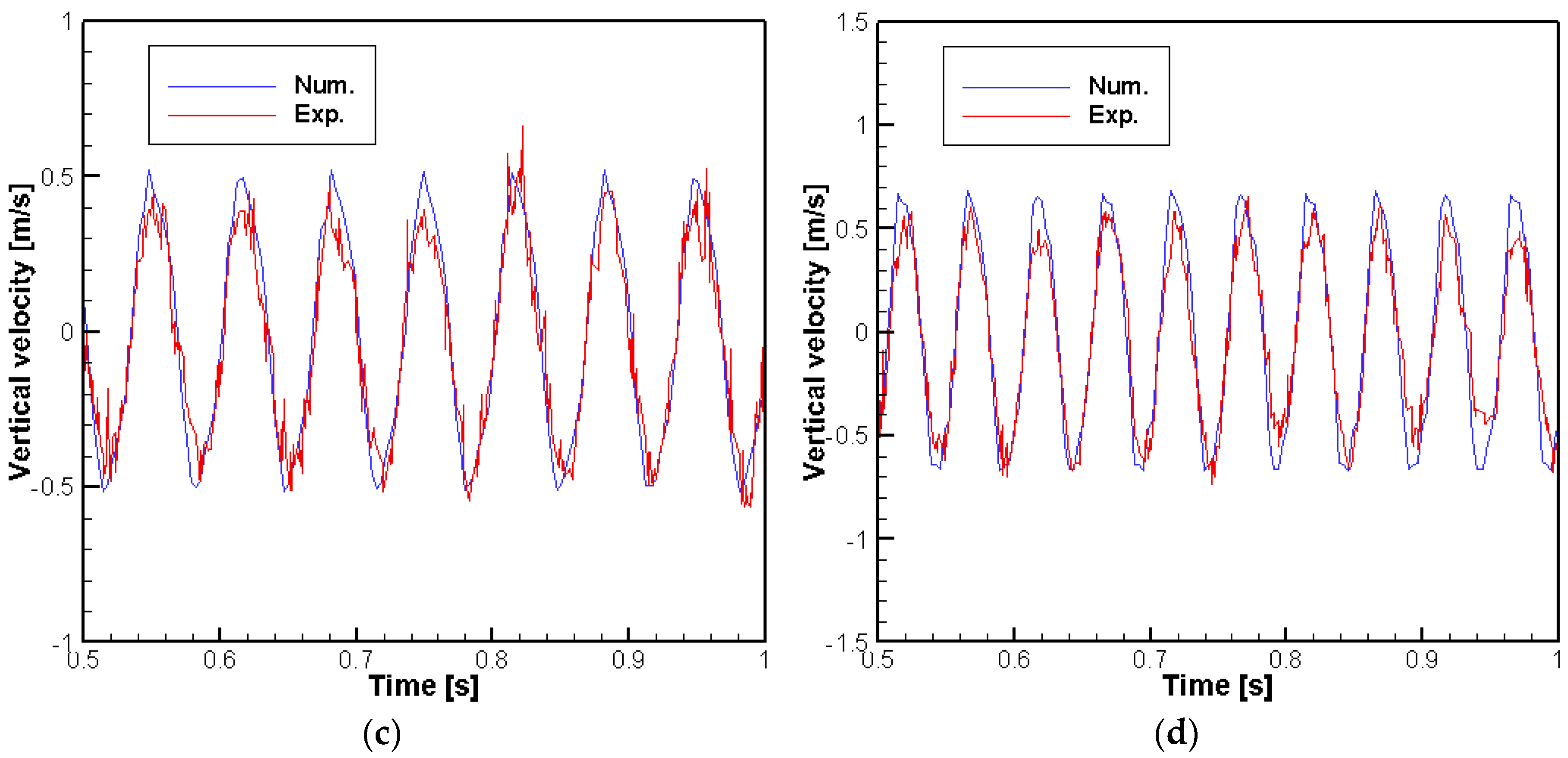
6. Gust Flow by Two Pitching Hydrofoils

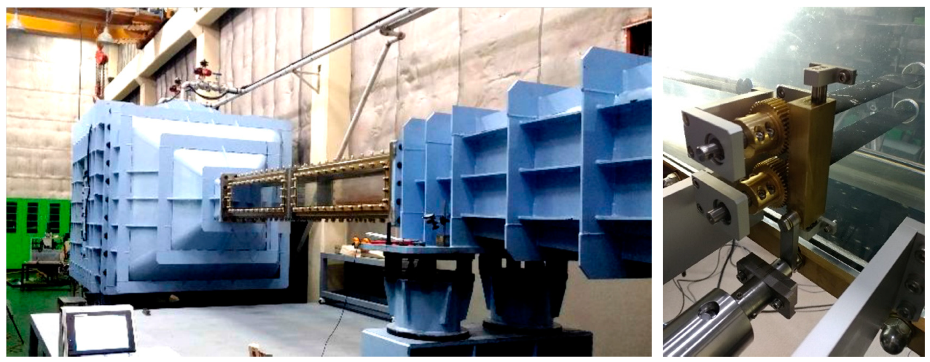
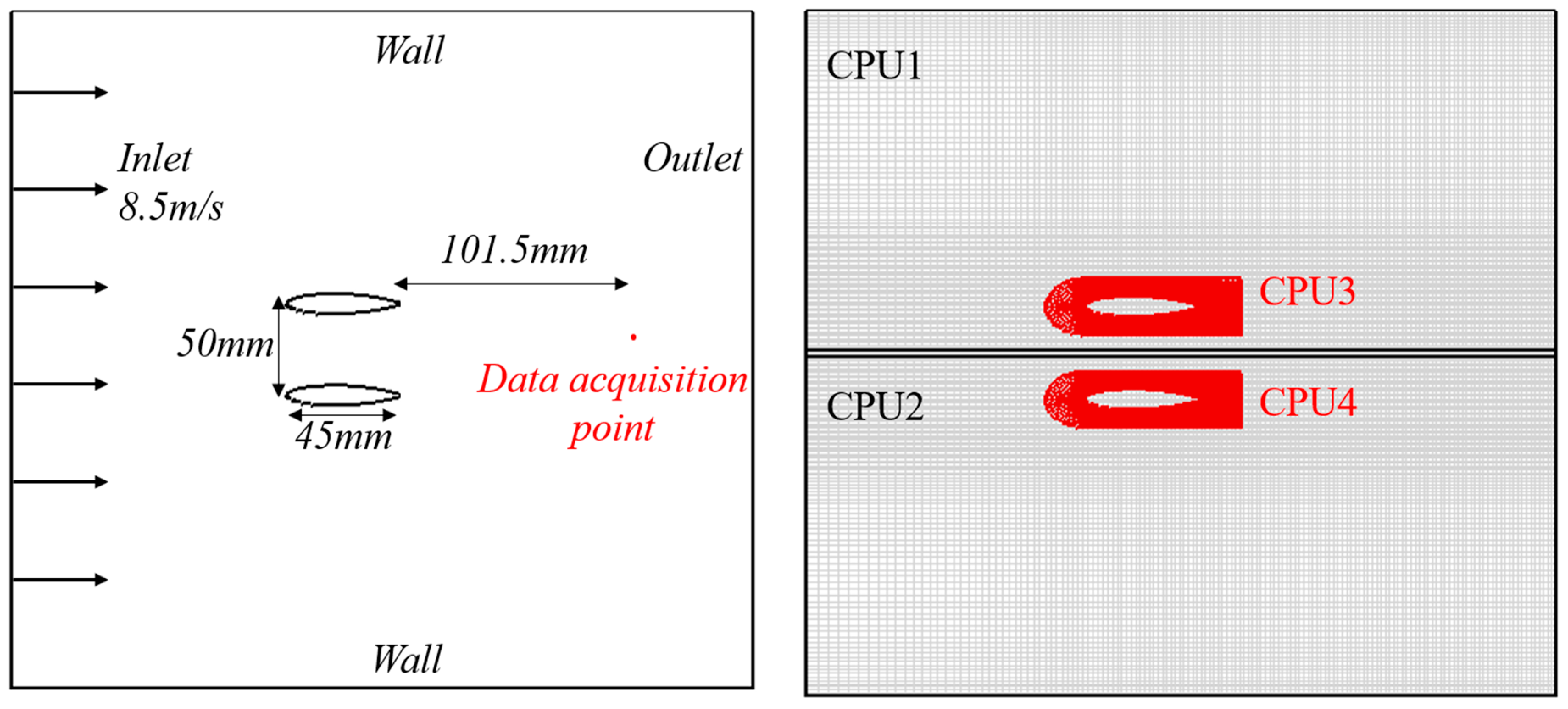
6.1. Experimental Setup and Computational Domain

Figure 18a shows the high-speed cavitation tunnel in the Korea Research Institute of Ships and Ocean Engineering (KRISO), where the experiment on gust flow was carried out. Figure 18b shows the gust generator consisting of twin hydrofoils with its driving system. The tunnel exhibits a rectangular test section with dimensions of 3000 mm (X) × 300 mm (Y) × 300 mm (Z), where the coordinates denotes the directions of main flow stream, the height, and the width, respectively. The flow velocity that is generated is up to 20.4 m/s [48]. The hydrofoil was used as the gust generator [1]. The gust generated by the twin hydrofoils is convected downstream at the mean flow velocity, oscillating at the prescribed frequencies. To measure the velocity of gust flow at the data acquisition point shown in Figure 19a, one-dimensional laser Doppler velocimetry (FlowExplorer 300 by Dantec Dynamics) was used with an uncertainty of 0.04% [49]. The data acquisition point is placed to be the center point between the trailing edge of the hydrofoil and the position of the head of a submerged projectile, which will be placed to investigate the effects of incoming gust on its cavitation shape in a future study. Figure 19a shows the entire computational domain, including the twin hydrofoils with the applied boundary conditions. The computation domain is constructed by using the two-dimensional section, of which the dimensions are 350 mm (X) × 300 (mm) (Y), where the length in the main flow direction is shortened for the reduction of numerical gust. The upper and lower boundaries are set as the solid wall on which no-slip boundary condition (BC) is applied. The left boundary is set as the inlet boundary on which the uniform velocity of 8.5 m/s in the horizontal direction is prescribed. The right boundary is set as the outlet boundary with the prescribed static pressure. The computational domain includes four domains (i.e., two background and two hydrofoil-fitted grid domains), as shown in Figure 19b. The hydrofoil-fitted grid domains oscillate in a pitching direction with prescribed amplitudes and frequencies corresponding to 4°, 6°, and 8°, and 5 Hz, 10 Hz, 15 Hz, and 20 Hz, respectively.

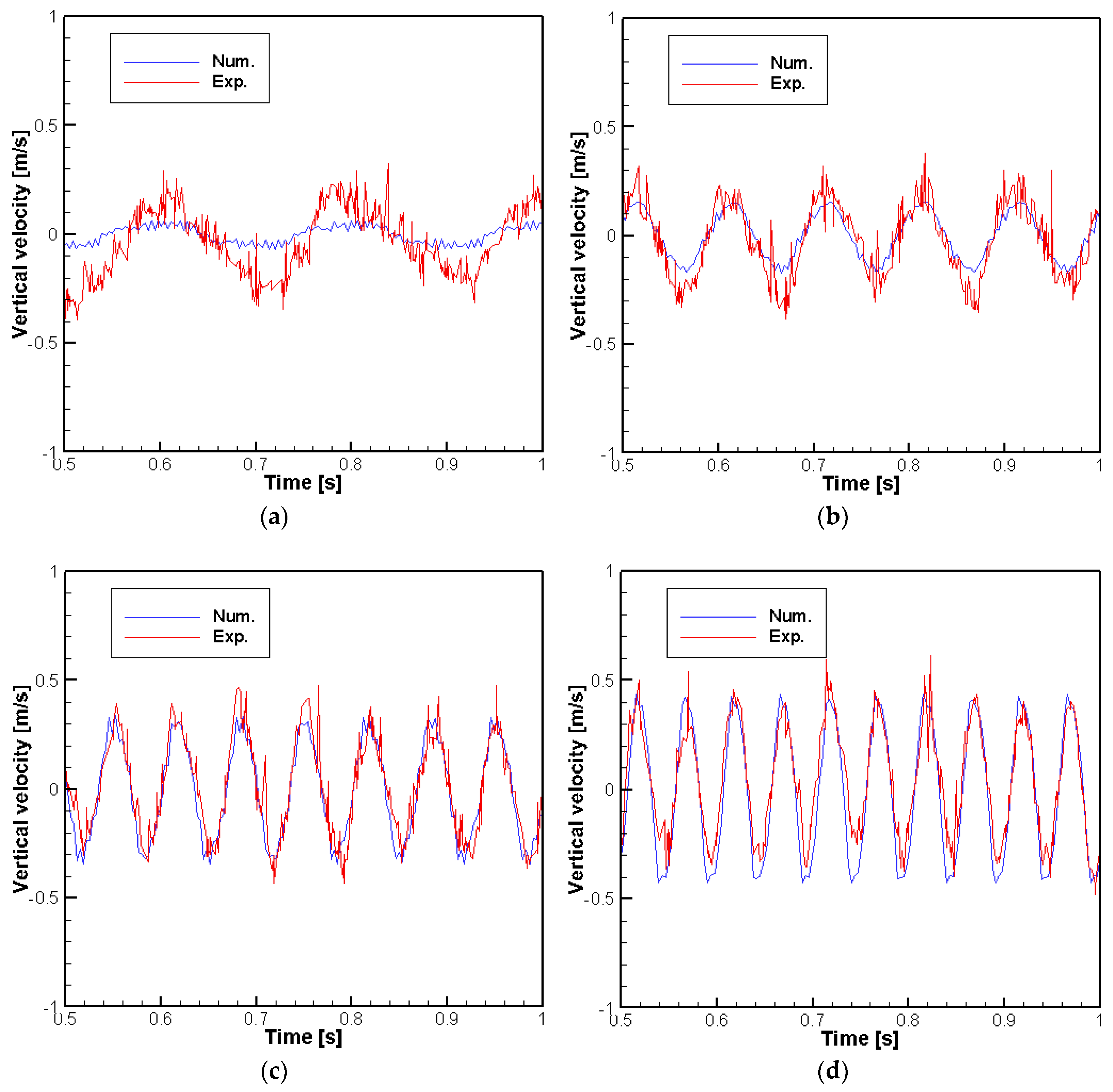
6.2. Numerical Results with Measured Data

Figure 20 shows the isocontours of pressure and u-velocity when the hydrofoils are positioned at the maximum angle of attacks. It can be seen that the gust flow generated by the twin hydrofoils is convected downstream smoothly without any discontinuity at the boundaries between the background and the subdomains.

Figure 21, Figure 22 and Figure 23 show the predicted time histories of the v-velocity component recorded at the data acquisition point due to the gust flow generated by the pitching hydrofoils at the amplitudes and frequencies as listed above. Periodic fluctuations in the velocity are observed in all of the cases. This implies that the twin pitching-hydrofoils successfully generate gust flow with periodic velocity components in a direction that is normal to the mean flow. In case of the 5-Hz frequency, a difference exists between the numerical and experimental results. This is because the oscillation frequency of the hydrofoils is extremely low, such that its wavelength is relatively long when compared with the size of the computational domain, and thus, the related vortical waves are increasingly affected by the boundary conditions. It is well known that any of the outflow boundary conditions do not work well for the low-frequency components of the wavelength comparable to the dimension of the entire computation domain [50]. In the present study, the lowest frequency of the vortical waves is 5 Hz, and the mean flow speed is 8.5 m/s, which results in the wavelength $\mathsf{\lambda }=8.5/5=1.7 \mathrm{m}$, which is much larger than the dimension of the computational domain. However, as the oscillation frequency increases, there are closer agreements between the numerical and the experimental results. To ensure the property of the current numerical scheme and preserve the dispersion relation, which is an important parameter for determining the ability of this numerical scheme to simulate wave-type phenomena, the numerical wave number of the present scheme needs to be analyzed [51,52,53,54,55,56]. The critical wavenumber can be defined as $|Im(k_{numer.c})\Delta x-k_{exact}\Delta x|=0.005$, according to which the critical wavenumber of the present scheme is $Im(k_{numer.c})\Delta x=\mathsf{\pi }/5$. This implies that the vortical wave satisfying the unequal equation $\mathrm{k}\Delta \mathrm{x}\le \mathsf{\pi }/5$ can be simulated using the proposed numerical scheme with negligible dispersion and dissipation errors. The grid for the part where the gust flow is generated is set to be 2 mm (X) × 1 mm (Y). Therefore, the present scheme can simulate the gust wave with a frequency of up to ${\mathrm{f}}_{\mathrm{c}}=u_{mean}\times k/2\pi =u_{mean}/10\Delta x=8.5/(10\times 0.002)=425 \mathrm{Hz}$. The results also indicate a similar trend wherein increases in the amplitude or the frequency increase the maximum velocity.

7. Conclusions

In the study, efficient and accurate parallel computation methods for two-phase flow problems involving complex moving foreign bodies were developed using the parallel computation based on the moving body-fitted grids overset on background multidomain meshes. First, the multiphase flow solver using the multidomain method with the grid-overlapping interface is validated. The solver was applied to predict the cavitation flow over a hemispherical head form, and its validity was confirmed by comparing its numerical results with the measured data. Subsequently, three types of interfaces boundary conditions, namely linear interpolation, two-point overlapped methods, and four-point overlapped methods were applied. It was theoretically and numerically demonstrated that parallel computation based on the four-point overlapped method provided almost the same numerical solution as serial computation. Next, the efficiency of the present parallel computation method was numerically investigated by varying the number of sub-blocks (or processors). When compared with the case of four blocks, the computation time was reduced by a factor of four, while the computational time was reduced 12 times in the case of 16 blocks. This indicates that the computation time did not decrease linearly with increases in the number of processors due to the overlapped grid points, wherein the total number of grid points increased when the number of the subdomain increased. However, the results indicated that multidomain approaches in combination with the four-point overlapping method can be used as accurate and efficient numerical tools to solve multiphase problems. Finally, the multidomain approaches were combined with moving overset grid techniques wherein the algorithm consisted of three sequential steps, namely hole-cutting, finding donor cells, and interpolation. The gust flow generated by twin pitching hydrofoils was numerically simulated using the present numerical method. The numerical results of the time histories of fluctuating vertical flow velocity indicated excellent agreement with the measured data in the considered range of the amplitudes and frequencies of the pitching motion of the hydrofoils. The results revealed that the present numerical method based on moving chimera grids in combination with the multidomain accurately and efficiently simulated the complex flow phenomena involving moving bodies. In the future study, the effects of incoming gust on cavitation flow around a high-speed submerged projectile will be investigated using the present numerical methods.

References

1. Kopriva, J.; Arndt, R.E.A.; Amromin, E.L. Improvement of hydrofoil performance by partial ventilated cavitation in steady flow and periodic gusts. J. Fluid Eng. 2008, 130, 031301. [Google Scholar] [CrossRef]
2. Lee, S.J.; Kawakami, E.; Arndt, R.E.A. Investigation of the Behavior of Ventilated Supercavities in a Periodic Gust Flow. J. Fluids Eng. 2013, 135, 081301. [Google Scholar] [CrossRef]
3. Lee, S.J.; Kawakami, E.; Karn, A.; Arndt, R.E.A. A comparative study of behaviors of ventilated supercavities between experimental models with different mounting configurations. Fluid Dyn. Res. 2016, 48, 045506. [Google Scholar] [CrossRef]
4. Karn, A.; Arndt, R.E.A.; Hong, J. Dependence of supercavity closure upon flow unsteadiness. Exp. Therm. Fluid Sci. 2015, 68, 493–498. [Google Scholar] [CrossRef] [Green Version]
5. Toumi, I.; Kumbaro, A.; Paillere, H. Approximate Riemann Solvers and Flux Vector Splitting Schemes for Two-Phase Flow; CEA Saclay, Direction de L’information Scientifique et Technique: Gif-sur-Yvette, France, 1999. [Google Scholar]
6. Hirt, C.W.; Nichols, B.D. Volume of fluid (VOF) method for the dynamics of free boundaries. J. Comput. Phys. 1981, 39, 201–225. [Google Scholar] [CrossRef]
7. Osher, S.; Sethian, J.A. Fronts propagating with curvature-dependent speed: Algorithms based on Hamilton–Jacobi formulations. J. Comput. Phys. 1988, 79, 12–49. [Google Scholar] [CrossRef]
8. Gingold, R.A.; Monaghan, J.J. Smoothed particle hydrodynamics - Theory and application to non-spherical stars. Mon. Not. R. Astron. Soc. 1977, 181, 375–389. [Google Scholar] [CrossRef]
9. Merkle, C.L.; Feng, J.; Buelow, P.E.O. Computational modeling of the dynamics of sheet cavitation. In Proceedings of the Third International Symposium on Cavitation, Grenoble, France, 7–10 April 1998; pp. 307–311. [Google Scholar]
10. Turkel, E. Preconditioned methods for solving the incompressible and low speed compressible equations. J. Comput. Phys. 1987, 72, 277–298. [Google Scholar] [CrossRef] [Green Version]
11. Choi, Y.-H.; Merkle, C.L. The application of preconditioning in viscous flows. J. Comput. Phys. 1993, 105, 207–223. [Google Scholar] [CrossRef]
12. Venkateswaran, S.; Merkle, C.L. Dual Time Stepping and Preconditioning for Unsteady Computations. In Proceedings of the 33rd Aerospace Sciences Meeting and Exhibit, Reno, NV, USA, 9–12 January 1995; p. 78. [Google Scholar]
13. Kunz, R.F.; Boger, D.A.; Chyczewski, T.S.; Stinebring, D.; Gibeling, H.; Govindan, T.R. Multi-phase CFD analysis of natural and ventilated cavitation about submerged bodies. In Proceedings of the 3rd ASME/JSME Joint Fluids Engineering Conference, FEDAM’99, San Francisco, CA, USA, 18–23 July 1999; Volume 99, p. 1. [Google Scholar]
14. Kunz, R.F.; Boger, D.A.; Stinebring, D.R.; Chyczewski, T.S.; Lindau, J.W.; Gibeling, H.J.; Venkateswaran, S.; Govindan, T.R. A preconditioned Navier–Stokes method for two-phase flows with application to cavitation prediction. Comput. Fluids 2000, 29, 849–875. [Google Scholar] [CrossRef]
15. Lindau, J.; Kunz, R.; Boger, D.; Stinebring, D.; Gibeling, H. Validation of high Reynolds number, unsteady multi-phase cfd modeling for naval applications. In Proceedings of the Twenty-Third Symposium on Naval Hydrodynamics, Val de Reuil, France, 17–22 September 2000. [Google Scholar]
16. Lindau, J.W.; Kunz, R.F.; Boger, D.A.; Stinebring, D.R.; Gibeling, H.J. High Reynolds number, unsteady, multiphase CFD modeling of cavitating flows. J. Fluids Eng. 2002, 124, 607–616. [Google Scholar] [CrossRef]
17. Owis, F.M.; Nayfeh, A.H. Numerical simulation of super-and partially-cavitating flows over an axisymmetric projectile. In Proceedings of the 39th Aerospace Sciences Meeting and Exhibit, Aerospace Sciences Meetings, Reno, NV, USA, 8–11 January 2001; p. 1042. [Google Scholar]
18. Owis, F.M.; Nayfeh, A.H. Numerical simulation of 3-D incompressible, multi-phase flows over cavitating projectiles. Eur. J. Mech. B Fluids 2004, 23, 339–351. [Google Scholar] [CrossRef]
19. Rouse, H.; McNown, J.S. Cavitation and Pressure Distribution: Head Forms at Zero Angle of Yaw; State University of Iowa: Iowa, CA, USA, 1948; p. 51. [Google Scholar]
20. Lindau, J.W.; Kunz, R.F.; Mulherin, J.M.; Dreyer, J.J.; Stinebring, D.R. Fully coupled, 6-DOF to URANS, modeling of cavitating flows around a supercavitating vehicle. In Proceedings of the 5th international symposium on cavitation, Osaka, Japan, 1–4 November 2003; pp. 1–4. [Google Scholar]
21. Venkateswaran, S.; Lindau, J.W.; Kunz, R.F.; Merkle, C.L. Preconditioning algorithms for the computation of multi-phase mixture flows. In Proceeding of the 39th Aerospace Sciences Meeting and Exhibit, Reno, NV, USA, 8–11 January 2001; p. 279. [Google Scholar]
22. Venkateswaran, S.; Lindau, J.W.; Kunz, R.F.; Merkle, C.L. Computation of multiphase mixture flows with compressibility effects. J. Comput. Phys. 2002, 180, 54–77. [Google Scholar] [CrossRef]
23. Ahuja, V.; Hosangadi, A.; Arunajatesan, S. Simulations of cavitating flows using hybrid unstructured meshes. J. Fluids Eng. 2001, 123, 331–340. [Google Scholar] [CrossRef]
24. Senocak, I.; Shyy, W. A pressure-based method for turbulent cavitating flow computations. J. Comput. Phys. 2002, 176, 363–383. [Google Scholar] [CrossRef]
25. Kunz, R.F.; Lindau, J.W.; Billet, M.L.; Stinebring, D.R. Multiphase CFD Modeling of Developed and Supercavitating Flows; Pennsylvania State University Applied Research Laboratory: Arlington, VA, USA, 2001. [Google Scholar]
26. Kunz, R.F.; Lindau, J.W.; Gibeling, H.J.; Mulherin, J.M.; Bieryla, D.J.; Reese, E.A. Unsteady, three-dimensional multiphase CFD analysis of maneuvering high speed supercavitating vehicles. In Proceedings of the 41st Aerospace Sciences Meeting and Exhibit, Reno, NV, USA, 6–9 January 2003; p. 841. [Google Scholar]
27. Lindau, J.W.; Venkateswaran, S.; Kunz, R.F.; Merkle, C.L. Development of a fully-compressible multi-phase Reynolds-averaged Navier-Stokes model. In Proceedings of the 15th AIAA Computational Fluid Dynamics Conference, Anaheim, CA, USA, 11–14 June 2001; p. 2648. [Google Scholar]
28. Lindau, J.W.; Venkateswaran, S.; Kunz, R.F.; Merkle, C.L. Computation of compressible multiphase flows. In Proceedings of the 41st Aerospace Sciences Meeting and Exhibit, Aerospace Sciences Meetings, Reno, NV, USA, 6–9 January 2003; p. 1285. [Google Scholar]
29. Lindau, J.W.; Venkateswaran, S.; Kunz, R.F.; Merkle, C.L. Multiphase computations for underwater propulsive flows. In Proceedings of the 16th AIAA Computational Fluid Dynamics Conference, Orlando, FL, USA, 23–26 June 2003; p. 4105. [Google Scholar]
30. Owis, F.M.; Nayfeh, A.H. Computations of the compressible multiphase flow over the cavitating high-speed torpedo. J. Fluids Eng. 2003, 125, 459–468. [Google Scholar] [CrossRef]
31. Kim, S.; Cheong, C.; Park, W.G. Numerical investigation on cavitation flow of hydrofoil and its flow noise with emphasis on turbulence models. AIP Adv. 2017, 7, 065114. [Google Scholar] [CrossRef] [Green Version]
32. Kim, S.; Cheong, C.; Park, W.-G. Numerical Investigation into Effects of Viscous Flux Vectors on Hydrofoil Cavitation Flow and Its Radiated Flow Noise. Appl. Sci. 2018, 8, 289. [Google Scholar] [Green Version]
33. Prewitt, N.C.; Belk, D.M.; Shyy, W. Parallel computing of overset grids for aerodynamic problems with moving objects. Prog. Aerosp. Sci. 2000, 36, 117–172. [Google Scholar] [CrossRef]
34. Stagg, A.K.; Carey, G.F.; Cline, D.D.; Shadid, J.N. Massively parallel MIMD solution of the parabolized Navier-Stokes equations. In Proceedings of the Scalable High Performance Computing Conference SHPCC-92, Williamsburg, VA, USA, 26–29 April 1992; pp. 328–335. [Google Scholar]
35. Ha, C.T.; Park, W.G. Evaluation of a new scaling term in preconditioning schemes for computations of compressible cavitating and ventilated flow. Ocean Eng. 2016, 126, 432–466. [Google Scholar] [CrossRef]
36. Ha, C.T.; Kim, D.H.; Park, W.G.; Jung, C.M. A compressive interface-capturing scheme for computation of compressible multi-fluid flows. Comput. Fluids 2017, 152, 164–181. [Google Scholar] [CrossRef]
37. Launder, B.E.; Spalding, D.B. The numerical computation of turbulent flows. In Numerical Prediction of Flow, Heat Transfer, Turbulence and Combustion; Elsevier: Amsterdam, The Netherlands, 1983; pp. 96–116. [Google Scholar]
38. Johansen, S.T.; Wu, J.; Shyy, W. Filter-based unsteady RANS computations. Int. J. Heat Fluid Flow 2004, 25, 10–21. [Google Scholar] [CrossRef] [Green Version]
39. Beam, R.M.; Warming, R.F. An implicit finite-difference algorithm for hyperbolic systems in conservation-law form. J. Comput. Phys. 1976, 22, 87–110. [Google Scholar] [CrossRef]
40. Van Leer, B. Towards the ultimate conservative difference scheme. V. A second-order sequel to Godunov’s method. J. Comput. Phys. 1979, 32, 101–136. [Google Scholar] [CrossRef]
41. Nguyen, V.T.; Vu, D.T.; Park, W.G.; Jung, C.M. Navier-Stokes solver for water entry bodies with moving Chimera grid method in 6DOF motions. Comput. Fluids 2016, 140, 19–38. [Google Scholar] [CrossRef]
42. Shen, Z.; Wan, D.; Carrica, P.M. Dynamic overset grids in OpenFOAM with application to KCS self-propulsion and maneuvering. Ocean Eng. 2015, 108, 287–306. [Google Scholar] [CrossRef]
43. Li, Y.; Paik, K.J.; Xing, T.; Carrica, P.M. Dynamic overset CFD simulations of wind turbine aerodynamics. Renewable Energy 2012, 37, 285–298. [Google Scholar] [CrossRef]
44. Carrica, P.M.; Wilson, R.V.; Noack, R.W.; Stern, F. Ship motions using single-phase level set with dynamic overset grids. Comput. Fluids 2007, 36, 1415–1433. [Google Scholar] [CrossRef]
45. Hsiao, C.T.; Chahine, G. Prediction of tip vortex cavitation inception using coupled spherical and nonspherical bubble models and Navier–Stokes computations. J. Mar. Sci. Technol. 2004, 8, 99–108. [Google Scholar] [CrossRef]
46. Graham, R.L. An efficient algorithm for determining the convex hull of a finite planar set. Inf. Process. Lett. 1972, 1, 132–133. [Google Scholar] [CrossRef]
47. Press, W.H.; Teukolsky, S.A.; Vetterling, W.T.; Flannery, B.P. Numerical Recipes in FORTRAN, 2nd ed.; Cambridge University Press: New York, NY, USA, 1992; Chapter 3; pp. 116–117. [Google Scholar]
48. Paik, B.G.; Park, I.R.; Kim, K.S.; Lee, K.C.; Kim, M.J.; Kim, K.Y. Design of a bubble collecting section in a high speed water tunnel for ventilated supercavitation experiments. J. Mech. Sci. Technol. 2017, 31, 4227–4235. [Google Scholar] [CrossRef]
49. Lee, S.J.; Paik, B.G.; Kim, K.Y.; Jung, Y.R.; Kim, M.J.; Arndt, R.E.A. On axial deformation of ventilated supercavities in closed-wall tunnel experiments. Exp. Therm. Fluid Sci. 2018, 96, 321–328. [Google Scholar] [CrossRef]
50. Tam, C.K.W.; Webb, J.C. Dispersion-relation-preserving finite difference schemes for computational acoustics. J. Comput. Phys. 1993, 107, 262–281. [Google Scholar] [CrossRef]
51. Cheong, C.; Lee, S. The effects of discontinuous boundary conditions on the directivity of sound from a piston. J. Sound Vib. 2001, 239, 423–443. [Google Scholar] [CrossRef]
52. Cheong, C.; Lee, S. Grid-optimized dispersion-relation-preserving schemes on general geometries for computational aeroacoustics. J. Com. Phys. 2001, 174, 248–276. [Google Scholar] [CrossRef]
53. Kim, D.; Cheong, C. Time- and frequency-domain computations of broadband noise due to interaction between incident turbulence and rectilinear cascade of fat plates. J. Sound Vib. 2012, 331, 4729–4753. [Google Scholar] [CrossRef]
54. Kim, D.; Heo, S.; Cheong, C. Time-domain inflow boundary condition for turbulence-airfoil interaction noise prediction using synthetic turbulence modeling. J. Sound Vib. 2015, 340, 138–151. [Google Scholar] [CrossRef]
55. Kim, D.; Lee, G.-S.; Cheong, C. Inflow broadband noise from an isolated symmetric airfoil interacting with incident turbulence. J. Fluids Struct. 2015, 55, 428–450. [Google Scholar] [CrossRef]
56. Kim, S.; Cheong, C.; Park, J.; Kim, H.; Lee, H. Investigation of flow and acoustic performances of suction mufflers in hermetic reciprocating compressor. Int. J. Refrig. 2016, 69, 74–84. [Google Scholar] [CrossRef]
Figure 1. Computational domain for serial and parallel computing.
Applsci 08 01937 g001
Figure 2. Data exchange at overlapped grids in the interface boundary.
Applsci 08 01937 g002
Figure 3. Subdomains with linear interpolation at five points (without overlapped points).
Applsci 08 01937 g003
Figure 4. Subdomains with two overlapped points.
Applsci 08 01937 g004
Figure 5. Subdomains with four overlapped points.
Applsci 08 01937 g005
Figure 6. Computation domain and associated boundary conditions.
Applsci 08 01937 g006
Figure 7. Grids used for serial and parallel computations; (a) single domain, (b) linear interpolation, (c) two-point overlapped, (d) four-point overlapped.
Applsci 08 01937 g007
Figure 8. Contours of water volume fraction at t* = 30; (a) single domain, (b) linear interpolation, (c) two-point overlapped, (d) four-point overlapped.
Applsci 08 01937 g008
Figure 9. Comparison of the mean pressure coefficients with respect to the overlapped methods for the interface boundary with the measured data: (a) total length; (b) peak value part.
Applsci 08 01937 g009
Figure 10. Contours of pressure around the interface boundary at t* = 30; (a) single block, (b) linear interpolation, (c) two-point overlapped, (d) four-point overlapped.
Applsci 08 01937 g010
Figure 11. Computation domains; (a) single block, (b) four blocks, (c) eight blocks, and (d) 16 blocks.
Applsci 08 01937 g011
Figure 12. Iso-contours of water volume fraction at t* = 30; (a) one block, (b) four blocks, (c) eight blocks, and (d) 16 blocks.
Applsci 08 01937 g012
Figure 13. Distribution of mean pressure coefficient based on the number of blocks: (a) total length; (b) peak value part.
Applsci 08 01937 g013
Figure 14. Performance of parallel computation based on the number of sub-blocks or processors.
Applsci 08 01937 g014
Figure 15. Schematic view of method to determine hole points using the dot product.
Applsci 08 01937 g015
Figure 16. Graham’s scan to check the presence of point P in the donor cell.
Applsci 08 01937 g016
Figure 17. Bilinear interpolation for point P.
Applsci 08 01937 g017
Figure 18. Experimental set-up: (a) high-speed cavitation tunnel; (b) gust generators with driving devices.
Applsci 08 01937 g018
Figure 19. Computation domain with applied boundary conditions and background and hydrofoil fitted grid domains. (red: hydrofoil fitted grid, gray: background grid).
Applsci 08 01937 g019
Figure 20. Snap shot of pressure and u-velocity at maximum angle (8°) of hydrofoils: (a) pressure; (b) u-velocity (black line: hydrofoils).
Applsci 08 01937 g020
Figure 21. V-velocity based on non-dimensional time in case of an amplitude of 8°: (a) 5 Hz; (b) 10 Hz; (c) 15 Hz; and (d) 20 Hz.
Applsci 08 01937 g021
Figure 22. V-velocity based on non-dimensional time in case of amplitude of 6°: (a) 5 Hz; (b) 10 Hz; (c) 15 Hz; and (d) 20 Hz.
Applsci 08 01937 g022aApplsci 08 01937 g022b
Figure 23. V-velocity based on non-dimensional time in the case of amplitude of 4°: (a) 5 Hz; (b) 10 Hz; (c) 15 Hz; and (d) 20 Hz.
Applsci 08 01937 g023