A Novel Hybrid Boundary-Type Meshless Method for Solving Heat Conduction Problems in Layered Materials

Abstract

In this article, we propose a novel meshless method for solving two-dimensional stationary heat conduction problems in layered materials. The proposed method is a recently developed boundary-type meshless method which combines the collocation scheme from the method of fundamental solutions (MFS) with the collocation Trefftz method (CTM) to improve the applicability of the method for solving boundary value problems. Particular non-singular basis functions from cylindrical harmonics are adopted in which the numerical approximation is based on the superposition principle using the non-singular basis functions expressed in terms of many source points. For the modeling of multi-layer composite materials, we adopted the domain decomposition method (DDM), which splits the domain into smaller subdomains. The continuity of the flux and the temperature has to be satisfied at the interface of subdomains for the problem. The validity of the proposed method is investigated for several test problems. Numerical applications were also carried out. Comparison of the proposed method with other meshless methods showed that it is highly accurate and computationally efficient for modeling heat conduction problems, especially in heterogeneous multi-layer composite materials.

1. Introduction

Since the 1940s, the knowledge of using composite laminate materials in industry has improved significantly [1]. A variety of methods have been developed to deal with composite laminate materials, which make the subject of composite laminate materials a matured discipline in applied science at present. The industrial use of composite laminate materials is widespread because they have the advantages of their anisotropic nature, which allows the material to be applied to a variety of engineering applications. However, composite materials may fail if subjected to severe environments such as high temperatures, even though there is no external load applied to the composites [2]. Specifically, failure in layered composites is caused by thermal induced stresses which are generated at the interface between different materials because the temperature distribution in the composites is non-uniform or discontinuous [3]. In order to understand how thermal stress is generated and distributed in the layered composites, it is important to investigate the temperature distribution in the composite laminate materials. While the mechanical behavior of composite laminate materials has been explored for decades, studies on the heat conduction problems of layered composites using the meshless methods are less explored, which initiated this study.

In the past, many heat conduction problems in layered composites have been routinely solved by numerical methods such as the finite difference method [4,5,6], finite element method [7,8], finite volume method [9,10,11] and the boundary element method [12,13]. In contrast to mesh-based numerical methods, the meshless methods, which do not need the mesh generation and boundary integral have been proposed such as the analytical method [14], method of fundamental solutions (MFS) [15,16,17], boundary knot method (BKM) [18], collocation Trefftz method (CTM) [19,20,21], radial basis function collocation method (RBFCM) [22,23,24,25], element-free Galerkin method (EFG) [26], reproducing kernel particle method (RKPM) [27,28], modified polynomial expansion method [29], meshless local boundary integral equation method (LBIE) [30,31], and so on. Among these, boundary-type meshless methods have attracted considerable attention because of their simplicity. The CTM [32] is categorized as a boundary-type meshless method for the numerical solution of problems where approximate solutions are expressed as a truncated series of T-complete basis functions automatically satisfying governing equations. The use of the CTM is less widespread because the system of linear equations obtained from the Trefftz method is an ill-posed system [33]. On the other hand, the MFS is also a boundary-type meshless method for solving problems where the solutions are approximated by the fundamental solution which is expressed in terms of source points. The MFS requires placing source points outside the domain of the problem to avoid the effects of the singular characteristics of the fundamental solution; however, it often encounters difficulties such as finding an appropriate location for the source points [34,35,36].

In this study, we propose a novel hybrid boundary-type meshless method for solving two-dimensional stationary heat conduction problems in layered composite materials. The proposed method combines the collocation scheme from the MFS with the CTM to improve the applicability of both methods. Particular non-singular basis functions from the cylindrical harmonics are adopted in which the numerical solutions are approximated by superpositioning of the non-singular basis functions expressed in terms of many source points. For the modeling of multi-layer composite materials, we adopted the domain decomposition method (DDM) [37], which splits the domain into smaller subdomains that are intersected only at the interface between layers. For each subdomain, there exists an independent layer with its own thermal conductivity. The basic concept of the DDM for modeling composite materials is that the continuity of the flux and the temperature has to be satisfied at the interface of subdomains for the problem. The validity of the proposed method is investigated for several test problems. Numerical analysis is also carried out. The rest of this article is organized as follows. In Section 2, we describe the governing equation of two-dimensional stationary heat conduction problems. Section 3 is devoted to the formulation of the hybrid boundary-type meshless method. In Section 4, numerical analysis of several test problems were conducted to evaluate the performance of the proposed numerical scheme. Finally, our conclusions are presented in Section 5.

2. Problem Statement

Considering a two-dimensional domain, $\Omega$, enclosed by a boundary $\Gamma$, the governing equations of stationary heat conduction and boundary conditions can be expressed as follows:

$${\nabla }^{2}u(x)=0\mathrm{in}\Omega$$

(1)

and

$$u=g\mathrm{on}{\Gamma }_{\mathrm{D}}$$

(2)

$$\frac{\partial u}{\partial n}=f\mathrm{on}{\Gamma }_f$$

(3)

where $u$ denotes the temperature, $\nabla$ denotes the Laplace operator, $\Omega$ denotes the object domain under consideration, $n$ denotes the outward normal direction, $g$ denotes the boundary where the Dirichlet boundary condition is given, ${\Gamma }_{\mathrm{D}}$ denotes the Dirichlet boundary, and $f$ denotes the boundary where the Neumann boundary condition is given, and ${\Gamma }_N$ denotes the Neumann boundary.

3. Hybrid Boundary-Type Meshless Method for Modeling Heat Conduction Problems

In the polar coordinate system, the governing equation of the stationary heat conduction problems is shown as follows:

$$\frac{{\partial }^{2}u}{\partial {\rho }^2}+\frac{1}{\rho }\frac{\partial u}{\partial \rho }+\frac{1}{{\rho }^2}\frac{{\partial }^{2}u}{\partial {\theta }^2}=0$$

(4)

where $\rho$ is the radius and $\theta$ is the polar angle in the polar coordinate system. In the proposed method, the approximation is established via superpositioning a series of particular non-singular basis functions of the heat equation in terms of many source points located within the domain. An approximation solution of two-dimensional stationary heat conduction problems can be expressed as a linear combination of particular non-singular basis function with unknown coefficients, ${\mathbf{a}}_{j,k}$.

$$u(\mathbf{x})\approx {\displaystyle \sum _{j=1}^O{\displaystyle \sum _{k=1}^P{\mathbf{a}}_{j,k}\mathbf{H}}(x,y_j)}$$

(5)

where $\mathbf{x}=(\rho ,\theta )$ and $\mathbf{x}\in \partial \Omega$ is the spatial coordinate that is collocated on the boundary, $y_j=({\rho }_j,{\theta }_j)$ is the source point, $O$ is the number of source points, $P$ is the order of the particular non-singular basis function, ${\mathbf{a}}_{j,k}=[\begin{array}{cc}{c}_{jk}& d_{jk}\end{array}]$ is a vector of unknown coefficients to be determined, $\mathbf{H}(\mathbf{x},{\mathbf{y}}_j)$ is the selected combination of the particular solutions of the heat equation in the two-dimensional polar coordinate system. The particular non-singular basis function of the heat equation can be expressed as

$$\mathbf{H}(\mathbf{x},{\mathbf{y}}_j)={\left[\begin{array}{cc}{({\rho }_j/R)}^k\cos (k{\theta }_j)& ({{\rho }_j/R)}^k\sin (k{\theta }_j)\end{array}\right]}^T$$

(6)

In this study, we adopt the characteristic length [38] as

$$R=1.5\times \max (\rho )$$

(7)

where $\max (\rho )$ is the maximum radial distance in the problem domain. Applying the Dirichlet boundary condition, we obtain

$$u({\mathbf{x}}_l)\approx {\displaystyle \sum _{j=1}^O{\displaystyle \sum _{k=1}^P{\mathbf{a}}_{j,k}{\mathbf{H}}_{j,k}}({\mathbf{x}}_l,{\mathbf{y}}_j)}=g({\mathbf{x}}_l),l=1,\mathrm{...},Q$$

(8)

where $g({\mathbf{x}}_l)$ is the Dirichlet boundary value imposed at the boundary collocation point. $Q$ is the number of boundary collocation points. The Neumann boundary condition can be written as

$$\frac{\partial u({\mathbf{x}}_l)}{\partial n}=\frac{\partial u({\mathbf{x}}_l)}{\partial x}{n}_x+\frac{\partial u({\mathbf{x}}_l)}{\partial y}{n}_y$$

(9)

where

$$\frac{\partial u({\mathbf{x}}_l)}{\partial x}=\frac{\partial u({\mathbf{x}}_l)}{\partial \rho }\frac{\partial \rho }{\partial x}+\frac{\partial u({\mathbf{x}}_l)}{\partial \theta }\frac{\partial \theta }{\partial x}\mathrm{and}\frac{\partial u({\mathbf{x}}_l)}{\partial y}=\frac{\partial u({\mathbf{x}}_l)}{\partial \rho }\frac{\partial \rho }{\partial y}+\frac{\partial u({\mathbf{x}}_l)}{\partial \theta }\frac{\partial \theta }{\partial y}$$

(10)

where $n_x$ and $n_y$ are normal vectors in the $x$ and $y$ direction, respectively. $\partial u/\partial \rho$ and $\partial u/\partial \theta$ can be rewritten as follows:

$$\frac{\partial u({\mathbf{x}}_l)}{\partial \rho }={\displaystyle \sum _{j=1}^O{\displaystyle \sum _{k=1}^P{\mathbf{a}}_{j,k}{[\begin{array}{cc}k{(1/R)}^k{\rho }_j^{k-1}\cos (k{\theta }_j)& k{(1/R)}^k{\rho }_j^{k-1}\sin (k{\theta }_j)\end{array}]}^T}}$$

(11)

$$\frac{\partial u({\mathbf{x}}_l)}{\partial \theta }={\displaystyle \sum _{j=1}^O{\displaystyle \sum _{k=1}^P{\mathbf{a}}_{j,k}{[\begin{array}{cc}-k{(1/R)}^k{\rho }_j^k\sin (k{\theta }_j)& k{(1/R)}^k{\rho }_j^k\cos (k{\theta }_j)\end{array}]}^T}}$$

(12)

Inserting Equations (11) and (12) into Equation (9), we may obtain

$$\frac{\partial u({\mathbf{x}}_l)}{\partial n}={\displaystyle \sum _{j=1}^O{\displaystyle \sum _{k=1}^P{\mathbf{a}}_{j,k}{\left[\begin{array}{cc}\partial ({({\rho }_j/R)}^k\cos (k{\theta }_j))/\partial n& \partial ({({\rho }_j/R)}^k\sin (k{\theta }_j))/\partial n\end{array}\right]}^T}}$$

(13)

where

$$\frac{\partial ({({\rho }_j/R)}^k\cos (k{\theta }_j))}{\partial n}=\begin{array}{c}[(k{(1/R)}^k{\rho }_j^{k-1}\cos (k{\theta }_j)\cos {\theta }_j)+(k{(1/R)}^k{\rho }_j^{k-1}\sin (k{\theta }_j)\sin {\theta }_j)]n_x\\ +[(k{(1/R)}^k{\rho }_j^{k-1}\cos (k{\theta }_j)\sin {\theta }_j)-(k{(1/R)}^k{\rho }_j^{k-1}\sin (k{\theta }_j)\cos {\theta }_j)]n_y\end{array}$$

(14)

$$\frac{\partial ({({\rho }_j/R)}^k\sin (k{\theta }_j))}{\partial n}=\begin{array}{c}[(k{(1/R)}^k{\rho }_j^{k-1}\sin (k{\theta }_j)\cos {\theta }_j)-(k{(1/R)}^k{\rho }_j^{k-1}\cos (k{\theta }_j)\sin {\theta }_j)]n_x\\ +[(k{(1/R)}^k{\rho }_j^{k-1}\sin (k{\theta }_j)\sin {\theta }_j)+(k{(1/R)}^k{\rho }_j^{k-1}\cos (k{\theta }_j)\cos {\theta }_j)]n_y\end{array}$$

(15)

Applying the Neumann boundary condition, we obtain

$$\frac{\partial u({\mathbf{x}}_l)}{\partial n}\approx {\displaystyle \sum _{j=1}^O{\displaystyle \sum _{k=1}^P{\mathbf{a}}_{j,k}{\left[\begin{array}{cc}\partial ({({\rho }_j/R)}^k\cos (k{\theta }_j))/\partial n& \partial ({({\rho }_j/R)}^k\sin (k{\theta }_j))/\partial n\end{array}\right]}^T}}=f({\mathbf{x}}_l),l=1,\mathrm{...},Q$$

(16)

where $f({\mathbf{x}}_l)$ is the Neumann boundary value imposed at boundary collocation points. Using Equations (8) and (16), we obtain the following linear systems of the form:

$$\mathbf{A}\mathsf{\alpha }=\mathbf{b}$$

(17)

$$\mathbf{A}=\left[\begin{array}{ccccc}({\rho }_1/R)\cos ({\theta }_1)& ({\rho }_1/R)\sin ({\theta }_1)& ...& {({\rho }_1/R)}^k\cos (k{\theta }_1)& {({\rho }_1/R)}^k\sin (k{\theta }_1)\\ ({\rho }_2/R)\cos ({\theta }_2)& ({\rho }_2/R)\sin ({\theta }_2)& ...& {({\rho }_2/R)}^k\cos (k{\theta }_2)& {({\rho }_2/R)}^k\sin (k{\theta }_2)\\ ({\rho }_3/R)\cos ({\theta }_3)& ({\rho }_3/R)\sin ({\theta }_3)& ...& {({\rho }_3/R)}^k\cos (k{\theta }_3)& {({\rho }_3/R)}^k\sin (k{\theta }_3)\\ ⋮& ⋮& ...& ⋮& ⋮\\ ({\rho }_i/R)\cos ({\theta }_i)& ({\rho }_i/R)\sin ({\theta }_i)& ...& {({\rho }_i/R)}^k\cos (k{\theta }_i)& {({\rho }_i/R)}^k\sin (k{\theta }_i)\\ N_{1,k=1}^{\mathrm{I}}& N_{1,k=1}^{\mathrm{II}}& ...& N_{1,k=m}^{\mathrm{I}}& N_{1,k=m}^{\mathrm{II}}\\ N_{2,k=1}^{\mathrm{I}}& N_{2,k=1}^{\mathrm{II}}& ...& N_{2,k=m}^{\mathrm{I}}& N_{2,k=m}^{\mathrm{II}}\\ N_{3,k=1}^{\mathrm{I}}& N_{3,k=1}^{\mathrm{II}}& ...& N_{3,k=m}^{\mathrm{I}}& N_{3,k=m}^{\mathrm{II}}\\ ⋮& ⋮& ...& ⋮& ⋮\\ N_{j,k=1}^{\mathrm{I}}& N_{j,k=1}^{\mathrm{II}}& ...& N_{j,k=m}^{\mathrm{I}}& N_{j,k=m}^{\mathrm{II}}\end{array}\right],\mathsf{\alpha }=\left[\begin{array}{c}{a}_0\\ a_1\\ a_2\\ a_3\\ ⋮\\ ⋮\\ ⋮\\ a_{m-2}\\ a_{m-1}\\ a_m\end{array}\right],\mathbf{b}=\left[\begin{array}{c}{g}_1\\ g_2\\ g_3\\ ⋮\\ g_i\\ f_1\\ f_2\\ f_3\\ ⋮\\ f_j\end{array}\right]$$

(18)

where

$$N_{j,k}^{{\rm I}}={\displaystyle \sum _{j=1}^O{\displaystyle \sum _{k=1}^P\begin{array}{c}[(k{(1/R)}^k{\rho }_j^{k-1}\cos (k{\theta }_j)\cos {\theta }_j)+(k{(1/R)}^k{\rho }_j^{k-1}\sin (k{\theta }_j)\sin {\theta }_j)]n_x\\ +[(k{(1/R)}^k{\rho }_j^{k-1}\cos (k{\theta }_j)\sin {\theta }_j)-(k{(1/R)}^k{\rho }_j^{k-1}\sin (k{\theta }_j)\cos {\theta }_j)]n_y\end{array}}}$$

(19)

$$N_{j,k}^{\mathrm{I}\mathrm{I}}={\displaystyle \sum _{j=1}^O{\displaystyle \sum _{k=1}^P\begin{array}{c}[(k{(1/R)}^k{\rho }_j^{k-1}\sin (k{\theta }_j)\cos {\theta }_j)-(k{(1/R)}^k{\rho }_j^{k-1}\cos (k{\theta }_j)\sin {\theta }_j)]n_x\\ +[(k{(1/R)}^k{\rho }_j^{k-1}\sin (k{\theta }_j)\sin {\theta }_j)+(k{(1/R)}^k{\rho }_j^{k-1}\cos (k{\theta }_j)\cos {\theta }_j)]n_y\end{array}}}$$

(20)

where $\mathbf{A}$ is a matrix of particular non-singular basis function with the size of $Q\times S$, $S=(2P\times O)$, $Q$ is the number of boundary collocation points for given boundary conditions, $P$ is the order of the particular non-singular basis function, and $O$ is the number of source points. $\mathsf{\alpha }$ is a vector of unknown coefficients with the size of $S\times 1$, $\mathbf{b}$ is a vector of given values from boundary conditions at collocation points with the size of $Q\times 1$. $i\le Q$ and $j\le Q$ where $i$ is the number of boundary collocation points for Dirichlet boundary condition, $j$ is the number of boundary collocation points for Neumann boundary condition, $g_1,g_2,\mathrm{...},g_i$ are the values of the Dirichlet boundary condition, $f_1,f_2,\mathrm{...},f_j$ are the values of $\partial u/\partial n$ for the Neumann boundary condition. For simplicity, the commercial program MATLAB backslash operator was used to solve Equation (17).

For the modeling of multi-layer composite materials, we adopted the DDM [37]. The DDM splits the domain into smaller subdomains in which subdomains are intersected only at the interface between layers. For each subdomain, there exists an independent layer with its own thermal conductivity. The boundary and source points are collocated in each subdomain. At the interface, the boundary collocation points on the left and right sides coincide with each other. The basic concept of the DDM for modeling composite materials is that the subdomains intersecting at the interface must satisfy flux conservation and continuity of the temperature for the problem, so that flux and temperature at the interface between two consecutive layers remain the same. For instance, we consider a rectangular domain $\Omega$, which can be divided into two smaller subdomains, ${\Omega }_1$ and ${\Omega }_2$ as shown in Figure 1. In order to simulate the heat conduction problem, the rectangular domain is divided into ${\Gamma }_1$, ${\Gamma }_2$, …, ${\Gamma }_8$ sub-boundaries. At ${\Omega }_1$ subdomains, the sub-boundaries include ${\Gamma }_1$, ${\Gamma }_2$, ${\Gamma }_3$ and ${\Gamma }_4$; At ${\Omega }_2$ subdomains, the sub-boundaries include ${\Gamma }_5$, ${\Gamma }_6$, ${\Gamma }_7$ and ${\Gamma }_8$. As noted above, the sub-boundary at the interface should satisfy the flux conservation and continuity of the temperature between two consecutive materials. The additional boundary conditions at the interface can be expressed as

$${u|}_{{\Gamma }_2}={u|}_{{\Gamma }_6},{\frac{\partial u}{\partial n}|}_{{\Gamma }_2}={\frac{\partial u}{\partial n}|}_{{\Gamma }_6}$$

(21)

Matching the Dirichlet and Neumann boundary conditions on boundary collocation points, we may obtain the following simultaneous linear equations

$${\mathbf{A}}_{\mathrm{D}}{\mathsf{\alpha }}_{\mathrm{D}}={\mathbf{b}}_{\mathrm{D}}$$

(22)

$${\mathbf{A}}_{\mathrm{D}}=\left[\begin{array}{cc}{\mathbf{A}}_{{\Omega }_1}& {\mathbf{0}}_{{\Omega }_2}\\ {{\mathbf{A}}_{\mathrm{I}}|}_{{\Gamma }_2}& {{\mathbf{A}}_{\mathrm{I}}|}_{{\Gamma }_6}\\ {\mathbf{0}}_{{\Omega }_1}& {\mathbf{A}}_{{\Omega }_2}\end{array}\right],{\mathsf{\alpha }}_{\mathrm{D}}=\left[\begin{array}{c}{\mathsf{\alpha }}_{{\Omega }_1}\\ {\mathsf{\alpha }}_{{\Omega }_2}\end{array}\right],{\mathbf{b}}_{\mathrm{D}}=\left[\begin{array}{c}{\mathbf{b}}_{{\Omega }_1}\\ {\mathbf{b}}_{\mathrm{I}}\\ {\mathbf{b}}_{{\Omega }_2}\end{array}\right]$$

(23)

where ${\mathbf{A}}_{{\Omega }_1}$ with the size of $l_1\times P_1$ and ${\mathbf{A}}_{{\Omega }_2}$ with the size of $l_2\times P_2$ are the $\mathbf{A}$ matrix shown in Equation (18) for ${\Omega }_1$ and ${\Omega }_2$, respectively. $l_1$ and $l_2$ are the number of boundary collocation points for ${\Omega }_1$ and ${\Omega }_2$, respectively. $P_1$ and $P_2$ are the number of the terms related to the order of the particular non-singular basis function for ${\Omega }_1$ and ${\Omega }_2$, respectively. ${{\mathbf{A}}_{\mathrm{I}}|}_{{\Gamma }_2}$ of the boundary ${\Gamma }_2$ with the size of $l_{\mathrm{I}}\times P_1$ and ${{\mathbf{A}}_{\mathrm{I}}|}_{{\Gamma }_6}$ of the boundary ${\Gamma }_6$ with the size of $l_{\mathrm{I}}\times P_2$ are the $\mathbf{A}$ matrices at the interface. $l_{\mathrm{I}}$ is the number of boundary collocation points at the interface. ${\mathbf{0}}_{{\Omega }_1}$ and ${\mathbf{0}}_{{\Omega }_2}$ are zero matrices with the size of $l_2\times P_1$ and $l_1\times P_2$, respectively. ${\mathsf{\alpha }}_{{\Omega }_1}$ with the size of $P_1\times 1$ is a vector of unknown coefficient of ${\Omega }_1$, ${\mathsf{\alpha }}_{{\Omega }_2}$ with the size of $P_2\times 1$ is a vector of an unknown coefficient of ${\Omega }_2$. ${\mathsf{\alpha }}_{{\Omega }_1}$ and ${\mathsf{\alpha }}_{{\Omega }_2}$ are vectors of boundary values of ${\Omega }_1$ and ${\Omega }_2$, respectively. ${\mathbf{b}}_{\mathrm{I}}=\begin{array}{cc}[{\mathbf{0}}_{\mathrm{g}}& {\mathbf{0}}_{\mathrm{f}}\end{array}{]}^{\mathrm{T}}$, ${\mathbf{0}}_{\mathrm{g}}$ and ${\mathbf{0}}_{\mathrm{f}}$ are zero vectors with the size of $l_{\mathrm{I}}\times 1$ for Dirichlet and Neumann boundary conditions at the interface, respectively.

By solving the above simultaneous linear equations, we may obtain two sets of unknown coefficients, ${\mathbf{b}}_{{\Omega }_1}$ and ${\mathbf{b}}_{{\Omega }_2}$, for subdomains, ${\Omega }_1$ and ${\Omega }_2$, respectively. To obtain the temperature for subdomains, the inner collocation points in ${\Omega }_1$ and ${\Omega }_2$ must be placed. The temperature, $u$, at inner collocation points can then be found by Equation (5) using ${\mathbf{A}}_{{\Omega }_1}$ and ${\mathbf{b}}_{{\Omega }_1}$ for ${\Omega }_1$, as well as ${\mathbf{A}}_{{\Omega }_2}$ and ${\mathbf{b}}_{{\Omega }_2}$ for ${\Omega }_2$.

4. Numerical Examples

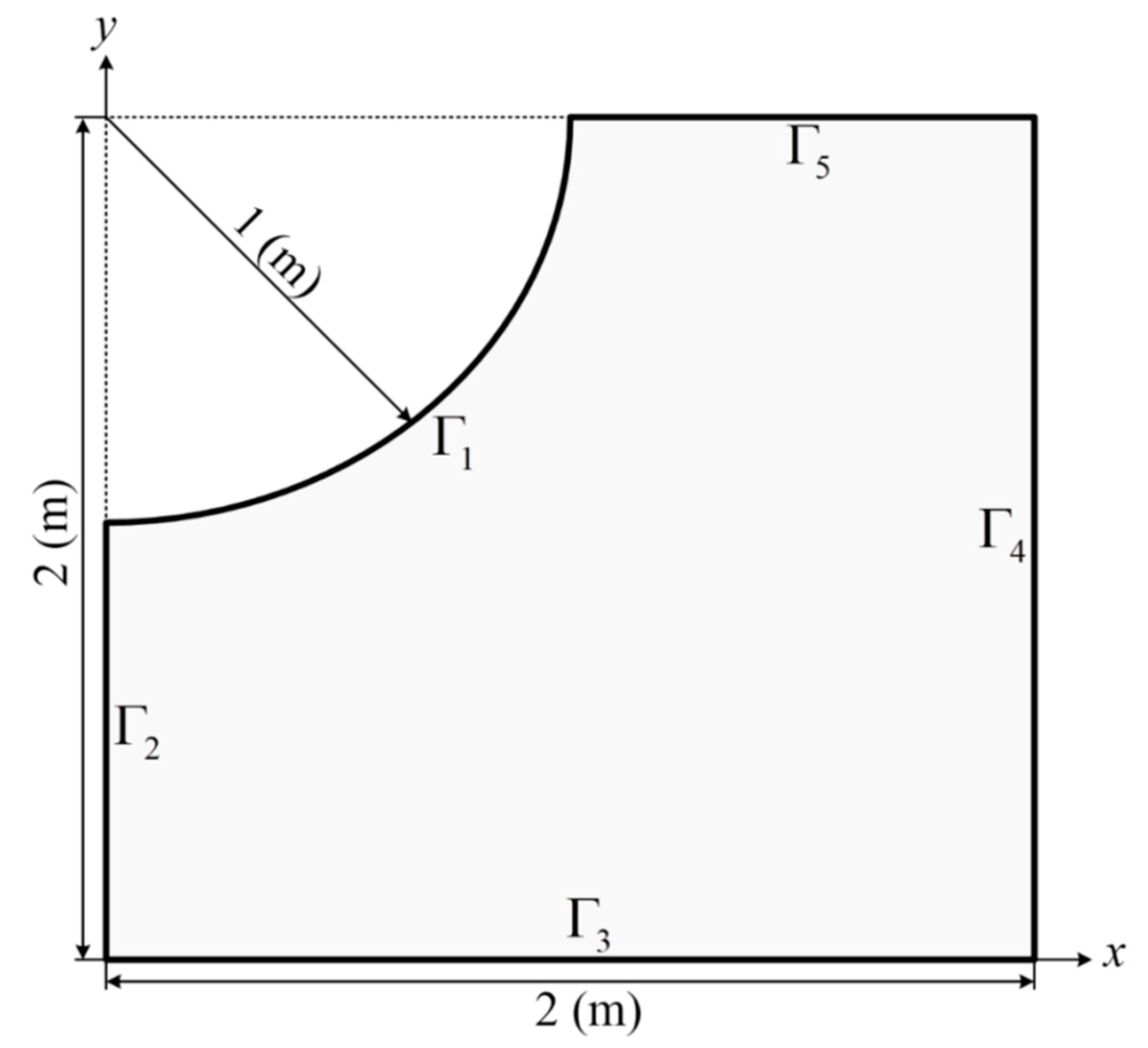
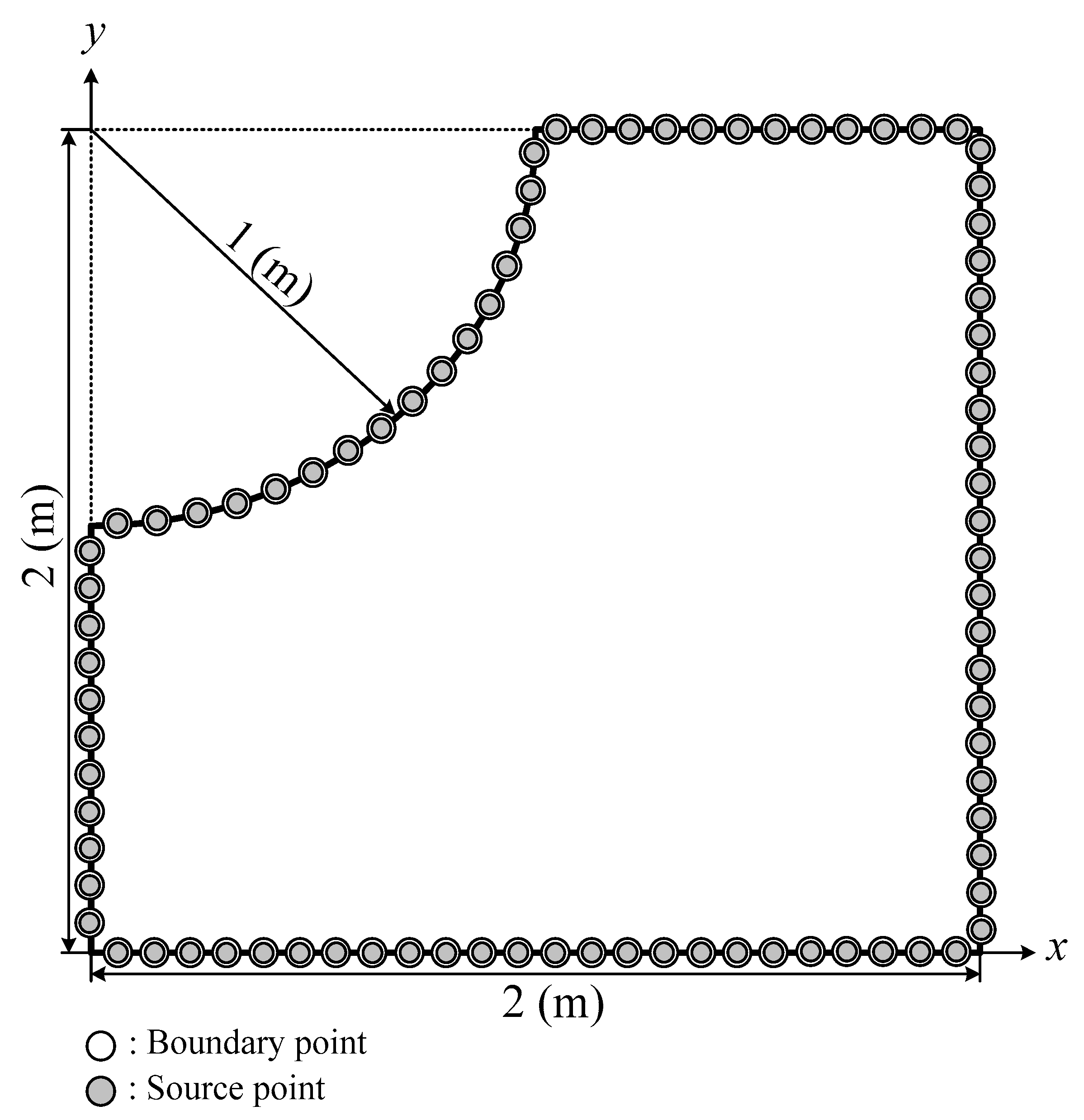
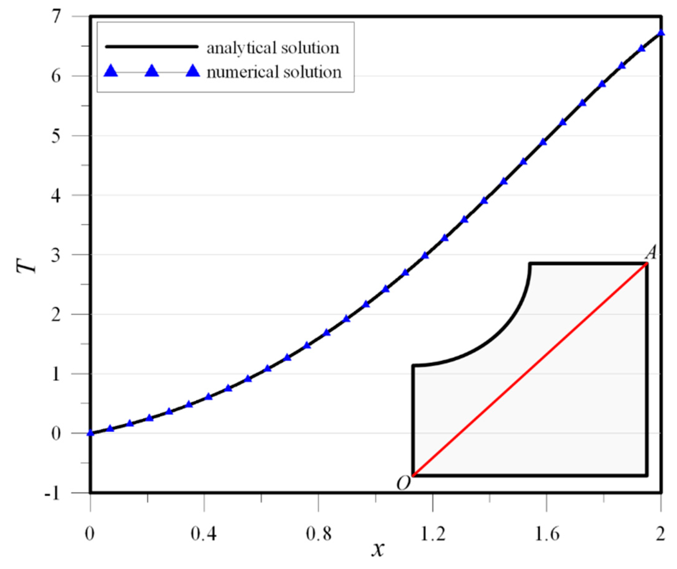
To validate the proposed hybrid boundary-type meshless method for modeling stationary heat conduction problems, several test problems were investigated during the simulation of heat conduction problems in composite materials and compared with the analytical solutions. In order to evaluate the accuracy of the numerical solution, we used the absolute and relative error as shown in the following equations.

$$\mathrm{Absolute} \mathrm{error}=u_{exact}(x_i)-u_{nu}(x_i)$$

(24)

$$\mathrm{Relative} \mathrm{error}=\sqrt{\frac{{(u_{exact}(x_i)-u_{nu}(x_i))}^2}{{(u_{exact}(x_i))}^2}}$$

(25)

where $u_{exact}(x_i)$ and $u_{nu}(x_i)$ are the exact and numerical solutions for the inner points $x_i$, respectively.

4.1. Example 1

The first scenario under investigation is a two-dimensional homogeneous isotropic stationary heat conduction problem [39], as shown in Figure 2. For a two-dimensional domain, $\Omega$, enclosed by an elliptical-shaped section, the governing equation of the heat conduction problem is expressed as follows:

$${\nabla }^{2}u(\mathbf{x})=0\mathrm{in}\Omega$$

(26)

The two-dimensional object boundary under consideration is defined as

$${\Gamma }_1=\left\{(x_1,y_1)|x_1{}^2/a^2+y_1{}^2/b^2=1\right\},a=2,b=1$$

(27)

$${\Gamma }_2=\left\{(x_2,y_2)|x_2=0,0\le y_2\le 1\right\}$$

(28)

$${\Gamma }_3=\left\{(x_3,y_3)|0\le x_3\le 2,y_3=0\right\}$$

(29)

The analytical solution may be found as

$$u=\frac{(b^2-a^2)xy}{a^2+b^2}$$

(30)

For solving this example, the order of the particular non-singular basis function $P$, is 15. The boundary condition is assumed to be the Dirichlet boundary condition using the analytical solution which is expressed as Equation (30) for the problem. The boundary and source points are uniformly distributed on the boundary for the hybrid boundary-type meshless method, as demonstrated in Figure 3. We compared the computed temperature of the inner collocation points in the computational domain with those from the analytical solution, as shown in Figure 4a. We obtained highly accurate numerical solutions in the order of 10⁻¹⁶ for this problem. Figure 4b demonstrates the accuracy of the element-free Galerkin method (EFG) [39] and the improved interpolating element-free Galerkin (IIEFG) method [39]. It is found that the accuracy of the EFG and the IIEFG methods can only reach the order of 10⁻¹⁶ for the same problem. Figure 5 shows the comparison of the computed results with the analytical solution of temperature along line AB. In addition, Figure 6 depicts a plot of the comparison of the computed temperature distribution with the analytical solution. From the figures, it can be seen that the numerical solution agrees very well with the analytical solution. This example shows that the proposed method may obtain more accurate results than the EFG and IIEFG methods.

4.2. Example 2

In order to verify the proposed hybrid boundary-type meshless method, we considered a homogeneous and isotropic example with a complex boundary shape. As shown in Figure 7, this example is a two-dimensional steady state heat conduction problem [39]. The governing equation of the example enclosed by $\Omega$ can be expressed as

$${\nabla }^{2}u(\mathbf{x})=0\mathrm{in}\Omega$$

(31)

The two-dimensional object boundary under consideration is defined as:

$${\Gamma }_1=\left\{(x_1,y_1)|x_1=\rho ({\theta }_1)\cos {\theta }_1,y_1=\rho ({\theta }_1)\sin {\theta }_1\right\},\rho ({\theta }_1)=1,0\le {\theta }_1\le 0.5\pi$$

(32)

$${\Gamma }_2=\left\{(x_2,y_2)|x_2=0,0\le y_2\le 1\right\}$$

(33)

$${\Gamma }_3=\left\{(x_3,y_3)|0\le x_3\le 2,y_3=0\right\}$$

(34)

$${\Gamma }_4=\left\{(x_4,y_4)|x_4=2,0\le y_4\le 2\right\}$$

(35)

$${\Gamma }_5=\left\{(x_5,y_5)|1\le x_5\le 2,y_5=2\right\}$$

(36)

The analytical solution may be found as

$$u=e^x\sin y$$

(37)

For solving this example, the order of the particular non-singular basis function $P$, is 15. The boundary condition is assumed to be the Dirichlet boundary condition using the analytical solution which is expressed as Equation (37). The boundary and source points are uniformly distributed on the boundary for the hybrid boundary-type meshless method, as demonstrated in Figure 8.

We first compared the computed temperature of the inner collocation points in the computational domain with those from the analytical solution, as shown in Figure 9a. We obtained highly accurate numerical solutions in the order of 10⁻¹¹ for this problem. Figure 9b demonstrates the accuracy of the element-free Galerkin method (EFG) [39] and the improved interpolating element-free Galerkin (IIEFG) method [39]. It was found that the accuracy of the EFG and the IIEFG methods can only reach to the order of 10⁻³ for the same problem. Figure 10 shows the comparison of the computed results with the analytical solution of temperature along line OA. In addition, Figure 11 depicts a plot of the comparison of the computed temperature distribution with the analytical solution. From these figures, it can be observed that the numerical solution agrees very well with the analytical solution. Again, this example shows that the proposed method may obtain more accurate results than the EFG and IIEFG methods.

4.3. Example 3

The third example under investigation is the modeling of two-dimensional isotropic stationary heat conduction problems in composite materials with a rectangular domain [40], as shown in Figure 1. The thermal conductivities in layer 1 and layer 2 are $1W/\mathrm{m}\mathrm{K}$ and $2W/\mathrm{m}\mathrm{K}$, respectively. For a two-dimensional domain, $\Omega$, enclosed by a rectangular boundary, the governing equation is expressed as follows:

$$\nabla (k(\mathbf{x})\nabla u(\mathbf{x}))=0\mathrm{in}\Omega$$

(38)

where $k$ denotes thermal conductivity. The two-dimensional object boundary under consideration is defined as

$${\Gamma }_1=\left\{(x_1,y_1)|-1\le x_1\le 1,0\le y_1\le 1\right\}$$

(39)

$${\Gamma }_2=\left\{(x_2,y_2)|-1\le x_2\le 1,0\le y_2\le -1\right\}$$

(40)

For the heat conduction equation, the analytical solution can be obtained as

$$u(x,y)=e^{-k_1/k_2(x^2-y^2)}\cos (2k_1/k_{2}xy)$$

(41)

where $k_1$ and $k_2$ are thermal conductivities in layer 1 and layer 2, respectively. The boundary and source points are uniformly distributed on the boundary, as demonstrated in Figure 12. For modeling the heat conduction problem in composite materials with a rectangular domain, the DDM [37] is adopted so that the domain boundary can be divide into several subdomains. Figure 1 shows that the two-dimensional object boundary is divided into several sub-boundaries: ${\Gamma }_1$, ${\Gamma }_2$, ${\Gamma }_3$, …, ${\Gamma }_8$. The Dirichlet boundary condition is imposed on the sub-boundaries using the analytical solution as shown in Equation (41) for the problem. At the interface, the sub-boundaries, including ${\Gamma }_2$ and ${\Gamma }_6$, should satisfy the flux conservation and the continuity of temperature. Therefore, the boundary conditions are given as follows:

$${u|}_{{\Gamma }_2}={u|}_{{\Gamma }_6},{\frac{\partial u}{\partial n}|}_{{\Gamma }_2}={\frac{\partial u}{\partial n}|}_{{\Gamma }_6}$$

(42)

In this example, we utilized the hybrid boundary-type meshless method for modeling heat conduction problems in composite materials with a rectangular domain. The reported CPU time is 1.67 seconds using the computer with Intel Core i7-7700 CPU at 3.60 GHz and the equipment is manufactured by the ASUSTeK Computer Inc., Taipei, Taiwan. To validate the accuracy of the proposed method, we collocated 1200 inner points inside the domain uniformly to obtain the solution of the temperature. Figure 13 demonstrates the comparison of the computed results with those from the analytical solution. It is found that the results agree very well with each other.

To evaluate the accuracy of the proposed method, the absolute error and relative error of the computed results with the analytical solution were calculated as shown in Figure 14. We obtained highly accurate numerical solutions in the order of 10⁻¹¹ for this problem. The singular boundary method [40] has been used to model the same problem. As shown in

Table 1. Comparison of computed results with those from references.

	This Study		Singular Boundary Method
	1st Layer	2nd Layer	1st Layer	2nd Layer
Maximum absolute error with the analytical solution	$2.74\times {10}^{-11}$	$3.25\times {10}^{-11}$	${10}^{-3}$	${10}^{-3}$
Maximum relative error with the analytical solution	$3.90\times {10}^{-11}$	$5.76\times {10}^{-11}$	${10}^{-3}$	${10}^{-3}$

, it was found that the accuracy of the singular boundary method for this example only reached to the order of 10⁻³.

4.4. Example 4

The fourth example under investigation is the modeling of two-dimensional isotropic stationary heat conduction problems of composite materials in a square domain with a hole [40], as depicted in Figure 15. The thermal conductivities in layer 1 and layer 2 are $1W/\mathrm{m}\mathrm{K}$ and $2W/\mathrm{m}\mathrm{K}$, respectively. In the first layer, two squares with sides f 2 and 20 around the boundary domain, respectively and the second layer is composed of two squares with sides of 20 and 60 around the boundary domain. For a two-dimensional domain, $\Omega$, enclosed by a boundary with a square domain, the governing equation is shown in Equation (38). The analytical solution can be obtained as

$$u(x,y)=k_1/k_2(x^2-y^2)$$

(43)

where $k_1$ and $k_2$ are thermal conductivities in layer 1 and layer 2, respectively. The boundary and source points are uniformly distributed on the boundary, as demonstrated in Figure 16. For modeling the heat conduction problem with composite materials, the DDM [37] was adopted so that the domain boundary can be divided into several subdomains. Figure 15 shows that the two-dimensional object boundary is divided into several sub-boundaries: ${\Gamma }_1$, ${\Gamma }_2$, ${\Gamma }_3$, …, ${\Gamma }_{16}$. The Dirichlet boundary condition is imposed on the sub-boundaries using the analytical solution for the problem, as shown in Equation (43). At the interface, the sub-boundaries, including ${\Gamma }_5$, ${\Gamma }_6$, ${\Gamma }_7$, ${\Gamma }_8$, ${\Gamma }_9$, ${\Gamma }_{10}$, ${\Gamma }_{11}$ and ${\Gamma }_{12}$, should satisfy the flux conservation and the continuity of temperature. Therefore, the boundary conditions are given as follows.

$${u|}_{{\Gamma }_5}={u|}_{{\Gamma }_9},{\frac{\partial u}{\partial n}|}_{{\Gamma }_5}={\frac{\partial u}{\partial n}|}_{{\Gamma }_9},{u|}_{{\Gamma }_6}={u|}_{{\Gamma }_{10}},{\frac{\partial u}{\partial n}|}_{{\Gamma }_6}={\frac{\partial u}{\partial n}|}_{{\Gamma }_{10}}$$

(44)

$${u|}_{{\Gamma }_7}={u|}_{{\Gamma }_{11}},{\frac{\partial u}{\partial n}|}_{{\Gamma }_7}={\frac{\partial u}{\partial n}|}_{{\Gamma }_{11}},{u|}_{{\Gamma }_8}={u|}_{{\Gamma }_{12}},{\frac{\partial u}{\partial n}|}_{{\Gamma }_8}={\frac{\partial u}{\partial n}|}_{{\Gamma }_{12}}$$

(45)

The reported CPU time was 18.00 s using the Intel Core i7-7700 CPU at 3.60 GHz. To examine the accuracy of the proposed method, we collocated 5445 inner points inside the domain uniformly to obtain the solution of the temperature. The computed temperature distribution of the inner points is depicted in Figure 17. It was found that the computed results agree very well with those from the analytical solution. To evaluate the accuracy of the proposed method, the absolute error and relative error of the computed results with the analytical solution were calculated as shown in Figure 18. We obtained highly accurate numerical solutions in the order of 10⁻⁷ and 10⁻¹¹ for the absolute error and relative error, respectively. The singular boundary method [40] was used to model the same problem. As shown in

Table 2. Comparison of computed results with those from references.

	This Study		Singular Boundary Method
	1st Layer	2nd Layer	1st Layer	2nd Layer
Maximum absolute error with the analytical solution	$6.30\times {10}^{-7}$	$8.16\times {10}^{-9}$	${10}^{-3}$	${10}^{-3}$
Maximum relative error with the analytical solution	$1.57\times {10}^{-7}$	$1.84\times {10}^{-10}$	${10}^{-4}$	${10}^{-5}$

, it was found that the accuracy of the singular boundary method for this example can only reach to the order of 10⁻³.

4.5. Example 5

In order to verify the hybrid boundary-type meshless method, we considered a more complex boundary shape with an irregular domain by comparing the results with the analytical solution. The fifth scenario investigated is similar to the fourth scenario, but it involved a more complex boundary shape, as depicted in Figure 19. The thermal conductivities in layer 1 and layer 2 are $1W/\mathrm{m}\mathrm{K}$ and $2W/\mathrm{m}\mathrm{K}$, respectively. The governing equation of Example 5 is expressed in Equation (35). Considering a boundary with an irregular shape, we may write the equations of the two-dimensional boundary as follows:

$${\Gamma }_1=\left\{(x_1,y_1)|x_1=\rho ({\theta }_1)\cos {\theta }_1,y_1=\rho ({\theta }_1)\sin {\theta }_1\right\},\rho ({\theta }_1)=2(\mathrm{abs}(\cos (0.5{\theta }_1{))}^{\sin ({\theta }_1)}),0\le {\theta }_1\le 2\pi$$

(46)

$${\Gamma }_2=\left\{(x_2,y_2)|-10\le x_2\le 10,y_2=10\right\}$$

(47)

$${\Gamma }_3=\left\{(x_3,y_3)|x_3=-10,-10\le y_3\le 10\right\}$$

(48)

$${\Gamma }_4=\left\{(x_4,y_4)|-10\le x_4\le 10,y_4=10\right\}$$

(49)

$${\Gamma }_5=\left\{(x_5,y_5)|x_5=10,-10\le y_5\le 10\right\}$$

(50)

$${\Gamma }_{10}=\left\{(x_{10},y_{10})|x_{10}=\rho ({\theta }_{10})\cos {\theta }_{10},y_{10}=\rho ({\theta }_{10})\sin {\theta }_{10}\right\},\rho ({\theta }_{10})=20(e^{(\sin {\theta }_{10}\sin 2{\theta }_{10})}{}^2+e^{(\cos {\theta }_{10}\cos 2{\theta }_{10})}{}^2),0\le {\theta }_{10}\le 2\pi$$

(51)

For the heat conduction equation, the analytical solution can be obtained as

$$u(x,y)=k_1/k_2(x^2-y^2)$$

(52)

where $k_1$ and $k_2$ are thermal conductivities in layer 1 and layer 2, respectively. The boundary and source points are uniformly distributed on the boundary, as demonstrated in Figure 20. For modeling the heat conduction problem with composite materials, the DDM [37] was adopted so that the domain boundary can be divided into several subdomains. Figure 19 shows that the two-dimensional object boundary was divided into several sub-boundaries: ${\Gamma }_1$, ${\Gamma }_2$, ${\Gamma }_3$, …, ${\Gamma }_{10}$. The Dirichlet boundary condition was imposed on the sub-boundaries using the analytical solution as shown in Equation (52). At the interface, the sub-boundaries, including ${\Gamma }_2$, ${\Gamma }_3$, ${\Gamma }_4$, ${\Gamma }_5$, ${\Gamma }_6$, ${\Gamma }_7$, ${\Gamma }_8$ and ${\Gamma }_9$, should satisfy the flux conservation and the continuity of temperature. Therefore, the boundary conditions are given as follows:

$$u_{{\Gamma }_2}={u|}_{{\Gamma }_6},{\frac{\partial u}{\partial n}|}_{{\Gamma }_2}={\frac{\partial u}{\partial n}|}_{{\Gamma }_6},{u|}_{{\Gamma }_3}={u|}_{{\Gamma }_7},{\frac{\partial u}{\partial n}|}_{{\Gamma }_3}={\frac{\partial u}{\partial n}|}_{{\Gamma }_7}$$

(53)

$${u|}_{{\Gamma }_4}={u|}_{{\Gamma }_8},{\frac{\partial u}{\partial n}|}_{{\Gamma }_4}={\frac{\partial u}{\partial n}|}_{{\Gamma }_8},{u|}_{{\Gamma }_5}={u|}_{{\Gamma }_9},{\frac{\partial u}{\partial n}|}_{{\Gamma }_5}={\frac{\partial u}{\partial n}|}_{{\Gamma }_9}$$

(54)

To examine the accuracy of the proposed method, we uniformly collocated 4984 inner points inside the domain to obtain the solution of the temperature. The computed temperature distribution of the inner points is depicted in Figure 21. It was found that the computed results agree very well with those from the analytical solution. To evaluate the accuracy of the proposed method, the absolute error and relative error of the computed results with the analytical solution were calculated, as shown in Figure 22. We obtained highly accurate numerical solutions in the order of ${10}^{-10}$ and ${10}^{-11}$ for the absolute error and relative error, respectively.

5. Discussion

In the CTM, the T-complete functions have to be derived by finding the general solutions of the governing equation. The solutions are expressed as a series using the linear combination of the T-complete functions. Since the T-complete functions satisfy the governing equation, we may place the boundary collocation points only on the boundary of the domain. In addition, the source point of the CTM is only one. The CTM requires the evaluation of a coefficient for each term in the series. On the other hand, the MFS adopts the fundamental solutions as its basis function. Since the fundamental solution has only one term, the MFS has to collocate many source points outside the domain to construct its basis function as a series. The MFS also requires the evaluation of a coefficient for each term in the series. For the CTM, the ill-posedness is often found when higher order terms of the basis functions are used. For the MFS, there is only one basis function but it requires many source points. Although the MFS does not require higher order terms of basis functions, the position of the source points in the MFS, however, is very sensitive to the results due to the singular characteristic of the fundamental solution of the differential operator.

In this article, we propose a novel method using non-singular basis functions instead of the singular solution. The collocation scheme of the proposed method is similar to the MFS. The non-singular basis functions are adopted from the cylindrical harmonics. Due to the adoption of the non-singular basis function, the locations of the source points are not sensitive to the results. This proposed method resolves a major difficulty in the MFS for finding appropriate locations for source points. From the results of the numerical examples, the proposed method was found to be superior in accuracy.

For modeling heterogeneous multi-layer composite materials, the DDM is adopted. The idea of the DDM for modeling composite materials is that the subdomains intersecting at the interface must satisfy flux conservation and the continuity of the temperature for the problem. We successfully integrated the DDM into the hybrid boundary-type meshless method. Two examples of heat conduction problems in heterogeneous multi-layer composite materials were investigated. The results obtained from the examples reveal that the proposed method can be applied to heterogeneous multi-layer composite materials. In addition, the collocation scheme of the proposed hybrid boundary-type meshless method is relatively simple because we only need to place the collocation points on the boundary of the domain. This would be advantageous for engineering problems involving the design of irregular shapes in applied sciences.

6. Conclusions

This paper presents a study on solving two-dimensional stationary heat conduction problems in composite laminate materials using the novel hybrid boundary-type meshless method. The findings of this study are summarized as follows:

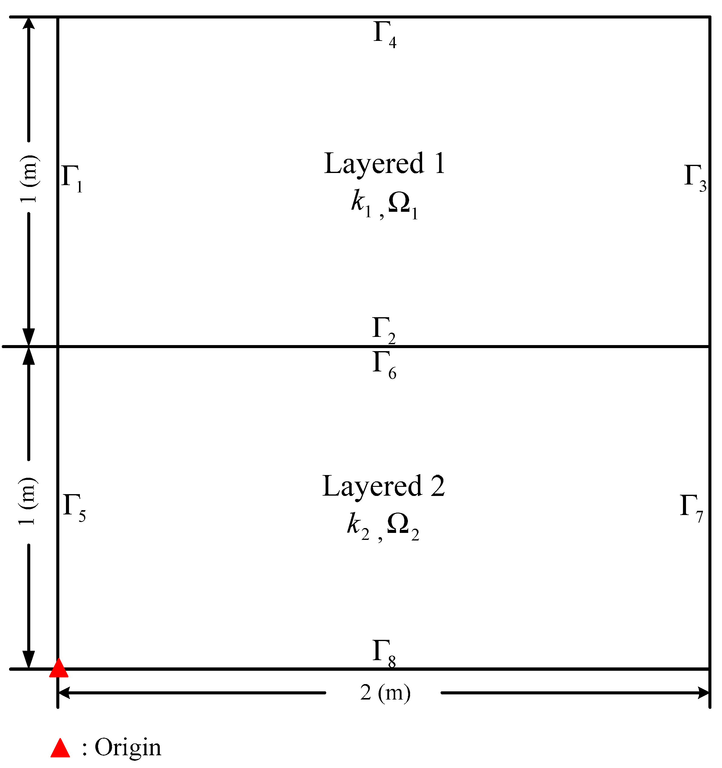
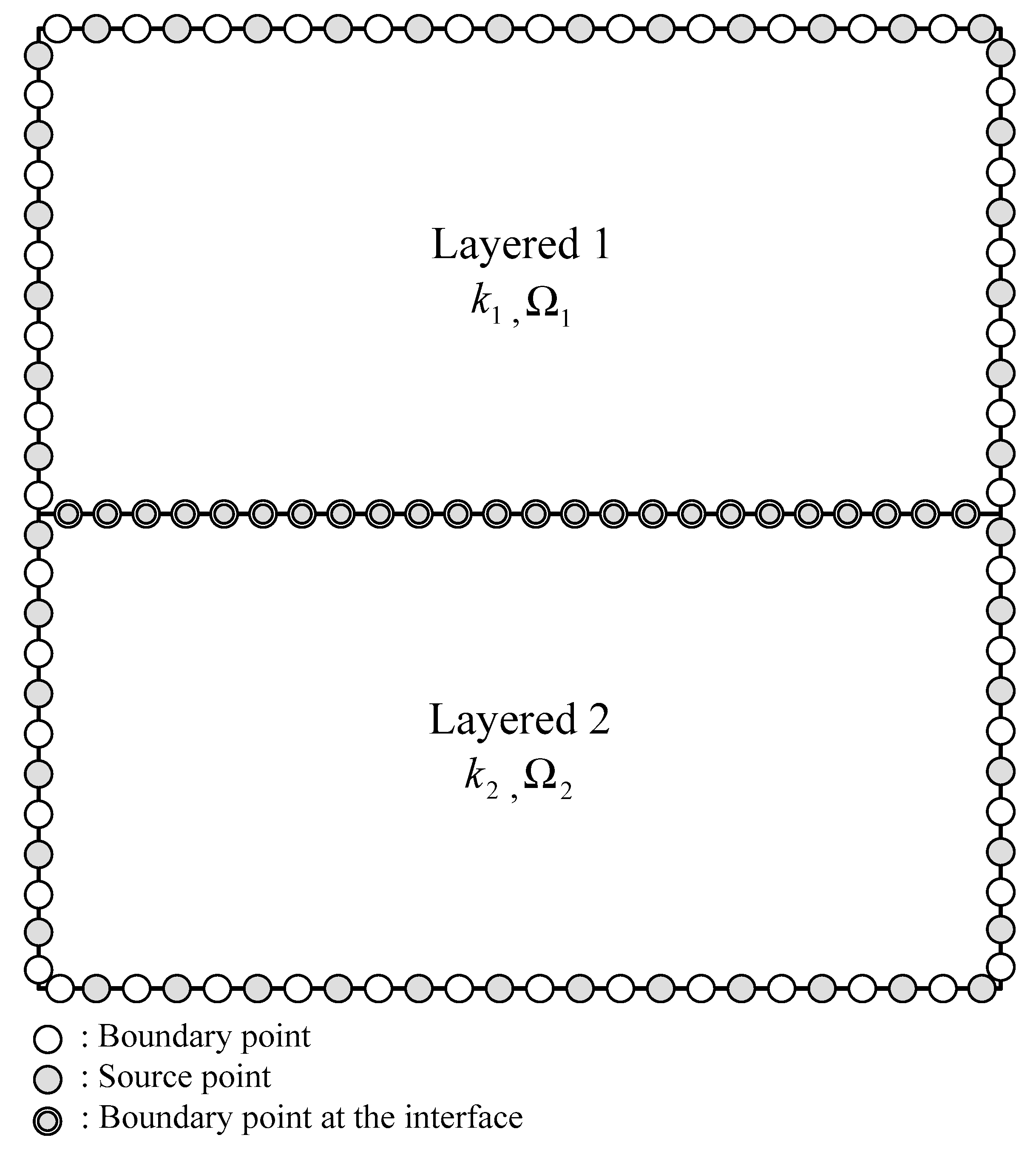
• Most applications of the boundary-type meshless method are still limited to homogeneous problems. This study presents pioneering work to investigate the numerical solutions of two-dimensional stationary heat conduction problems in layered heterogeneous composite materials using the novel boundary-type meshless method. We apply the DDM successfully for modeling composite materials in which the domain is split into smaller subdomains. The subdomains intersecting at the interface must satisfy flux conservation and the continuity of the temperature for the problem. It is found that the proposed method provides a promising solution for solving heat conduction problems with heterogeneity.
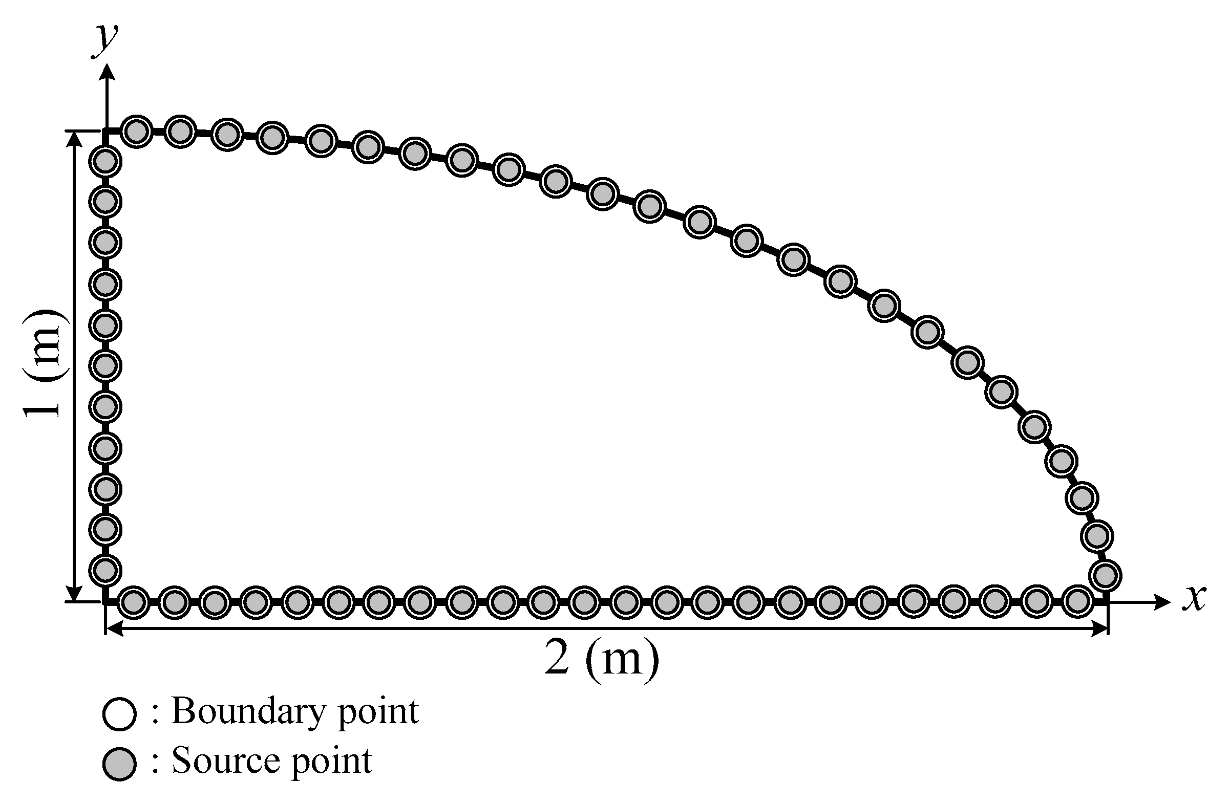
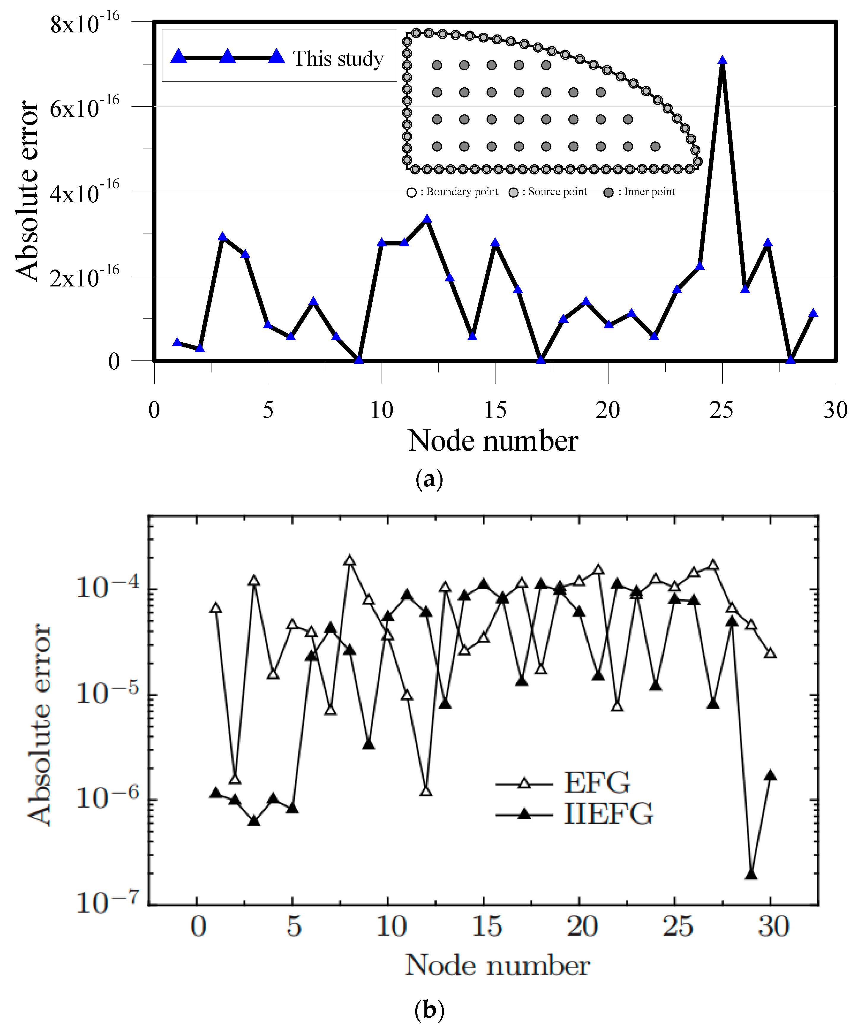
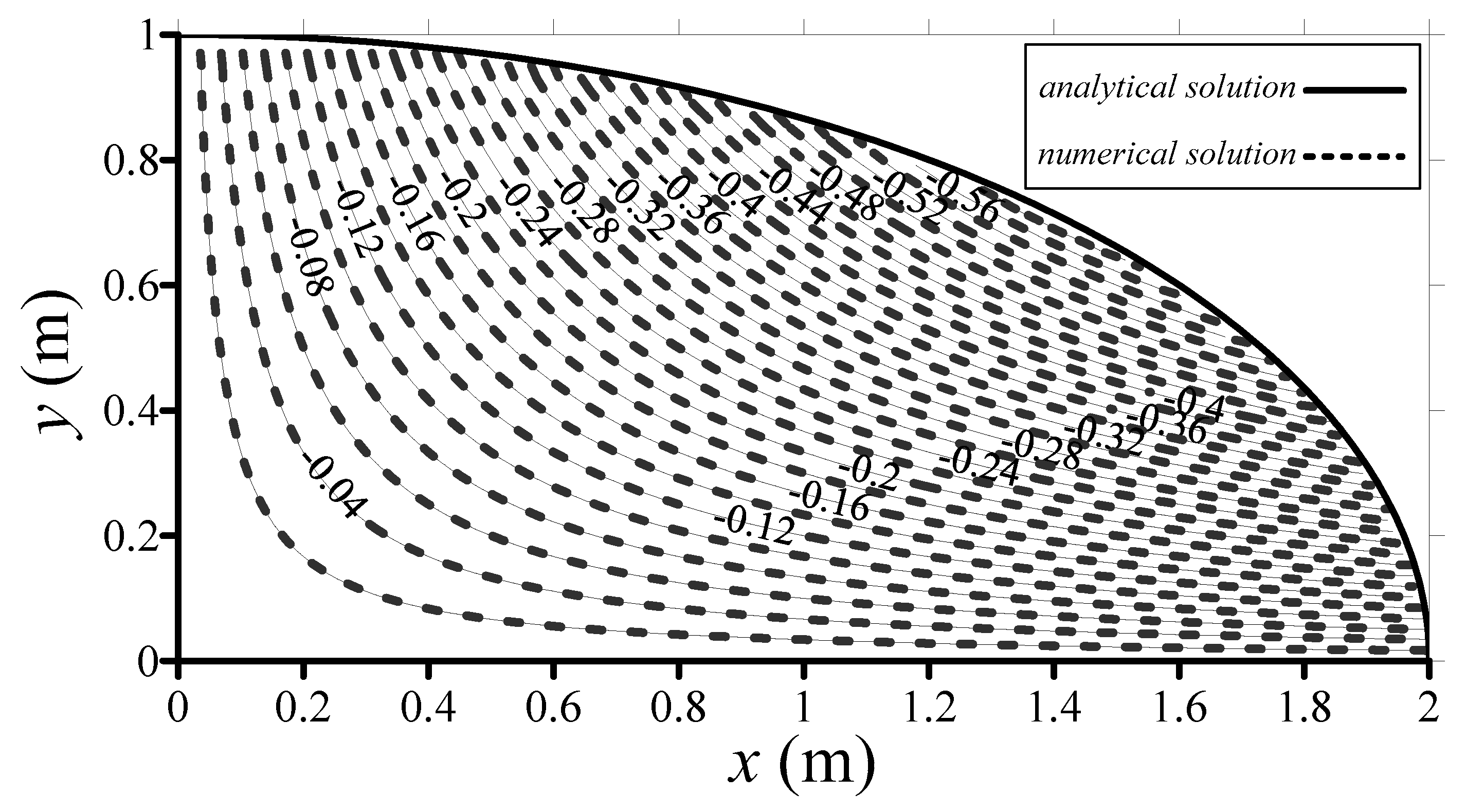
• In the proposed study, we only needed to place collocation points on the boundary. This demonstrated the advantages of the proposed boundary-type meshless method, including the boundary collocation only and high accuracy. Compared to the mesh-based approach, the proposed method is relatively simple and highly accurate. It is therefore advantageous for the analysis of heat conduction problems with a complex shape. Thus, the results obtained show that the proposed method is highly accurate and computationally efficient for modeling heat conduction problems, especially in heterogeneous multi-layer composite materials compared with other meshless methods. Nevertheless, the proposed method is still limited to problems with constant thermal conductivity. Future studies are suggested for problems involving nonlinear behavior.

References

1. Lubin, G. Handbook of Composites, 1st ed.; Van Norstrand Reinhold Publishing: New York, NY, USA, 1982. [Google Scholar]
2. Davies, P. Environmental degradation of composites for marine structures: New materials and new applications. Philos. Trans. R. Soc. Math. Phys. Eng. Sci. 2016, 374, 1–13. [Google Scholar] [CrossRef] [PubMed]
3. Yang, B.-F.; Yue, Z.-F.; Geng, X.-L.; Wang, P.-Y. Temperature effects on transverse failure modes of carbon fiber/bismaleimides composites. J. Compos. Mater. 2017, 51, 261–272. [Google Scholar] [CrossRef]
4. Wang, B.-L.; Han, J.-C.; Sun, Y.-G. A finite element/finite difference scheme for the non-classical heat conduction and associated thermal stresses. Finite Elem. Anal. Des. 2012, 50, 201–206. [Google Scholar] [CrossRef]
5. Wang, L.; Tian, F.-B. Heat transfer in non-Newtonian flows by a hybrid immersed boundary–Lattice Boltzmann and finite difference method. Appl. Sci. 2018, 8, 1–17. [Google Scholar] [CrossRef]
6. Chun, C.-K.; Park, S.-O. A Fixed-grid finite-difference method for phase-change problems. Numer. Heat Transf. Part B Fundam. 2000, 38, 59–73. [Google Scholar]
7. Wang, B.-L. Transient one-dimensional heat conduction problems solved by finite element. Int. J. Mech. Sci. 2005, 47, 303–317. [Google Scholar] [CrossRef]
8. He, K.-F.; Yang, Q.; Xiao, D.-M.; Li, X.-J. Analysis of thermo-elastic fracture problem during aluminium alloy MIG welding using the extended finite element method. Appl. Sci. 2017, 7, 1–20. [Google Scholar] [CrossRef]
9. Li, W.; Yu, B.; Wang, X.; Wang, P.; Sun, S. A finite volume method for cylindrical heat conduction problems based on local analytical solution. Int. J. Heat Mass Transf. 2012, 55, 5570–5582. [Google Scholar] [CrossRef]
10. Hassanzadeh, P.; Raithby, G.-D. Finite-volume solution of the second-order radiative transfer equation: Accuracy and solution cost. Numer. Heat Transf. Part B Fundam. 2008, 53, 374–382. [Google Scholar] [CrossRef]
11. Yang, C.-Z.; Liu, G.-X.; Chen, C.-M.; Xu, M. Numerical simulation of temperature fields in a three-dimensional SiC crystal growth furnace with axisymmetric and spiral coils. Appl. Sci. 2018, 8, 1–12. [Google Scholar] [CrossRef]
12. DeSilva, S.-J.; Chan, C.-L. Coupled boundary element method and finite difference method for the heat conduction in laser processing. Appl. Math. Model. 2008, 32, 2429–2458. [Google Scholar] [CrossRef]
13. Gao, X.-W.; Wang, J. Interface integral BEM for solving multi-medium heat conduction problems. Eng. Anal. Bound. Elem. 2009, 33, 539–546. [Google Scholar] [CrossRef]
14. Huang, F.-K.; Chuang, M.-H.; Wang, G.-S.; Yeh, H.-D. Tide-induced groundwater level fluctuation in a U-shaped coastal aquifer. J. Hydrol. 2015, 530, 291–305. [Google Scholar] [CrossRef]
15. Kupradze, V.-D.; Aleksidze, M.-A. The method of functional equations for the approximate solution of certain boundary value problems. USSR Comput. Math. Math. Phys. 1964, 4, 82–126. [Google Scholar] [CrossRef]
16. Katsurada, M.; Okamoto, H. The collocation points of the fundamental solution method for the potential problem. Comput. Math. Appl. 1996, 31, 123–137. [Google Scholar] [CrossRef]
17. Chen, J.-T.; Wu, C.-S.; Lee, Y.-T.; Chen, K.-H. On the equivalence of the Trefftz method and method of fundamental solutions for Laplace and biharmonic equations. Comput. Math. Appl. 2007, 53, 851–879. [Google Scholar] [CrossRef]
18. Fu, Z.-J.; Xi, Q.; Chen, W.; Cheng, A. A boundary-type meshless solver for transient heat conduction analysis of slender functionally graded materials with exponential variations. Comput. Math. Appl. 2018, 76, 760–773. [Google Scholar] [CrossRef]
19. Kita, E.; Kamiya, N. Trefftz method: An overview. Adv. Eng. Softw. 1995, 24, 1–3. [Google Scholar] [CrossRef]
20. Kita, E.; Kamiya, N.; Iio, T. Application of a direct Trefftz method with domain decomposition to 2D potential problems. Eng. Anal. Bound. Elem. 1999, 23, 539–548. [Google Scholar] [CrossRef]
21. Lv, H.; Hao, F.; Wang, Y.; Chen, C.-S. The MFS versus the Trefftz method for the Laplace equation in 3D. Eng. Anal. Bound. Elem. 2017, 83, 133–140. [Google Scholar] [CrossRef]
22. Amaziane, B.; Naji, A.; Ouazar, D. Radial basis function and genetic algorithms for parameter identification to some groundwater flow problems. Comput. Mater. Contin. 2004, 1, 117–128. [Google Scholar]
23. Fasshauer, G.-E.; Zhang, J.-G. On choosing optimal shape parameters for RBF approximation. Numer. Algorithms 2007, 45, 345–368. [Google Scholar] [CrossRef]
24. Kansa, E.-J. Multiquadrics-a scattered data approximation scheme with applications to computational fluid-dynamics-I surface approximations and partial derivative estimates. Comput. Math. Appl. 1990, 19, 127–145. [Google Scholar] [CrossRef]
25. Kansa, E.-J. Multiquadrics-a scattered data approximation scheme with applications to computational fluid-dynamics-II solutions to parabolic, hyperbolic and elliptic partial differential equations. Comput. Math. Appl. 1990, 19, 147–161. [Google Scholar] [CrossRef]
26. Belytschko, T.; Lu, Y.-Y.; Gu, L. Element-free Galerkin methods. Int. J. Numer. Methods Eng. 1994, 37, 229–256. [Google Scholar] [CrossRef]
27. Liu, W.-K.; Jun, S.; Zhang, Y.-F. Reproducing kernel particle methods. Int. J. Numer. Methods Fluids 1995, 20, 1081–1106. [Google Scholar] [CrossRef]
28. Chen, J.-S.; Pan, C.; Wu, C.-T.; Liu, W.-K. Reproducing kernel particle methods for large deformation analysis of nonlinear structures. Comput. Methods Appl. Mech. Eng. 1996, 139, 195–227. [Google Scholar] [CrossRef]
29. Chang, C.-W.; Liu, C.-H.; Wang, C.-C. A modified polynomial expansion algorithm forsolving the steady-state Allen-Cahn equation forheat transfer in thin films. Appl. Sci. 2018, 8, 1–16. [Google Scholar] [CrossRef]
30. Zhu, T.; Zhang, J.; Atluri, S.-N. Meshless numerical method based on the local boundary integral equation (LBIE) to solve linear and non-linear boundary value problems. Eng. Anal. Bound. Elem. 1999, 23, 375–389. [Google Scholar] [CrossRef]
31. Sladek, J.; Sladek, V.; Atluri, S.-N. Local boundary integral equation (LBIE) method for solving problems of elasticity with nonhomogeneous material properties. Comput. Mech. 2000, 24, 456–462. [Google Scholar] [CrossRef]
32. Ku, C.-Y.; Kuo, C.-L.; Fan, C.-M.; Liu, C.-S.; Guan, P.-C. Numerical solution of three-dimensional Laplacian problems using the multiple scale Trefftz method. Eng. Anal. Bound. Elem. 2015, 24, 157–168. [Google Scholar] [CrossRef]
33. Liu, C.-S. Improving the Ill-conditioning of the Method of Fundamental Solutions for 2D Laplace Equation. Comput. Model. Eng. Sci. 2015, 24, 157–168. [Google Scholar]
34. Cisilino, A.-P.; Sensale, B. Application of a simulated annealing algorithm in the optimal placement of the source points in the method of the fundamental solutions. Comput. Mech. 2002, 28, 129–136. [Google Scholar] [CrossRef]
35. Nishimura, R.; Nishimori, K.; Ishihara, N. Determining the arrangement of fictitious charges in charge simulation method using genetic algorithms. J. Electrost. 2000, 49, 95–105. [Google Scholar] [CrossRef]
36. Chen, C.-S.; Karageorghis, A.; Li, Y. On choosing the location of the sources in MFS. Numer. Algorithms 2016, 72, 107–130. [Google Scholar] [CrossRef]
37. Young, D.-L.; Fan, C.-M.; Tsai, C.-C.; Chen, C.-W. The method of fundamental solutions and domain decomposition method for degenerate seepage flow net problems. J. Chin. Inst. Eng. 2006, 29, 63–73. [Google Scholar] [CrossRef]
38. Ku, C.-Y.; Xiao, J.-E.; Liu, C.-Y.; Yeih, W. On the accuracy of the collocation Trefftz method for solving two- and three-dimensional heat equations. Numer. Heat Transf. Part B Fundam. Int. J. Comput. Methodol. 2016, 69, 334–350. [Google Scholar] [CrossRef]
39. Wang, J.-F.; Sun, F.-X.; Cheng, Y.-M. An improved interpolating element-free Galerkin method with a nonsingular weight function for two-dimensional potential problems. Chin. Phys. B 2012, 21, 1–7. [Google Scholar] [CrossRef]
40. Zheng, B.; Lin, J.; Chen, W. Simulation of heat conduction problems in layered materials using the meshless singular boundary method. Eng. Anal. Bound. Elem. 2018, 2018, 1–7. [Google Scholar] [CrossRef]
Figure 1. The profile of the composite materials for the analysis.
Applsci 08 01887 g001
Figure 2. The configuration of the boundary condition.
Applsci 08 01887 g002
Figure 3. Illustration of collocation points for boundary and source points.
Applsci 08 01887 g003
Figure 4. Comparison of computed results of the proposed method. (a) Comparison of results with the analytical solution and (b) comparison of results with the EFG and the IIEFG methods.
Applsci 08 01887 g004
Figure 5. Comparison of temperature results with the analytical solution along line AB.
Applsci 08 01887 g005
Figure 6. Comparison of the temperature distribution with the analytical solution.
Applsci 08 01887 g006
Figure 7. The configuration of the boundary condition.
Applsci 08 01887 g007
Figure 8. Illustration of the collocation points for boundary and source points.
Applsci 08 01887 g008
Figure 9. Comparison of computed results of the proposed method. (a) Comparison of results with the analytical solution and (b) comparison of results with the EFG and the IIEFG methods.
Applsci 08 01887 g009
Figure 10. The comparison of the computed results with the analytical solution of temperature along line OA.
Applsci 08 01887 g010
Figure 11. Comparison of temperature distribution with the analytical solution.
Applsci 08 01887 g011
Figure 12. Illustration of the collocation of boundary and source points.
Applsci 08 01887 g012
Figure 13. The comparison of temperature distribution with the analytical solution.
Applsci 08 01887 g013
Figure 14. Accuracy of the proposed method (with the comparison of the analytical solution). (a) Absolute error in the first layer, (b) absolute error in the second layer, (c) relative error in the first layer, and (d) relative error in the second layer.
Applsci 08 01887 g014aApplsci 08 01887 g014b
Figure 15. The configuration of the boundary condition.
Applsci 08 01887 g015
Figure 16. Illustration of the collocation of boundary and source points.
Applsci 08 01887 g016
Figure 17. The comparison of temperature distribution with the analytical solution.
Applsci 08 01887 g017
Figure 18. Comparison of results with the analytical solution. (a) Absolute error in the first layer, (b) absolute error in the second layer, (c) relative error in the first layer, and (d) relative error in the second layer.
Applsci 08 01887 g018aApplsci 08 01887 g018b
Figure 19. The configuration of the boundary condition.
Applsci 08 01887 g019
Figure 20. Illustration of the collocation of boundary and source points.
Applsci 08 01887 g020
Figure 21. The comparison of temperature distribution with the analytical solution.
Applsci 08 01887 g021
Figure 22. Comparison of results with the analytical solution. (a) Absolute error in the first layer, (b) absolute error in the second layer, (c) relative error in the first layer and (d) relative error in the second layer.
Applsci 08 01887 g022