Effect of Surface Mass Loading on Geodetic GPS Observations

Abstract

We investigated the effect of mass loading (atmospheric, oceanic and hydrological loading (AOH)) on Global Positioning System (GPS) height time series from 30 GPS stations in the Eurasian plate. Wavelet coherence (WTC) was employed to inspect the correlation and the time-variable relative phase between the two signals in the time–frequency domain. The results of the WTC-based semblance analysis indicated that the annual fluctuations in the two signals for most sites are physically related. The phase asynchrony at the annual time scale between GPS heights and AOH displacements indicated that the annual oscillation in GPS heights is due to a combination of mass loading signals and systematic errors (AOH modelling errors, geophysical effects and/or GPS system errors). Moreover, we discuss the impacts of AOH corrections on GPS noise estimation. The results showed that not all sites have an improved velocity uncertainty due to the increased amplitude of noise and/or the decreased spectral index after AOH corrections. Therefore, the posterior mass loading model correction is potentially feasible but not sufficient.

1. Introduction

The strong annual oscillations in Global Positioning System (GPS) observations are known to be driven by the redistribution of environmental mass loading [1,2]. The atmospheric, oceanic and hydrological loading (AOH) is a load that is likely to be important [3,4,5]. Surface deformation is usually large enough to be monitored using the space geodetic techniques [6,7,8] and can cause a significant reduction in the accuracy of GPS observations [9,10,11]. Globally distributed surface mass variabilities can be estimated to a certain extent using the method of a mass loading model and Gravity Recovery and Climate Experiment (GRACE) technology [12,13]. Van Dam et al. [14] corrected 51 GPS sites in Europe with AOH derived from GRACE and found that only 10 GPS stations have a reduction in their root mean square (RMS) values. Compared to GRACE, the mass loading model can estimate the small-scale variability [15]. Recently, Jiang et al. [16] adjusted 233 globally distributed GPS sites by AOH derived from the mass loading model, provided by the Global Geophysical Fluid Center (GGFC). The results indicated that 64% of the stations underwent a decrease in their RMS values, although the reasons for the inconsistency between the mass loading displacements and GPS observations were not discussed in detail. Considering that the RMS analysis is only used in the time domain, wavelet coherence (WTC) is a useful exploratory tool to expose regions with high correlations and to further reveal the relative phases between two time series in the time and frequency domain. In this study, we adopted the mass loading model to correct GPS observations using RMS analysis and WTC. Moreover, we will discuss the effect of mass loading correction on site velocity uncertainty and noise estimation.

2. Materials and Methods

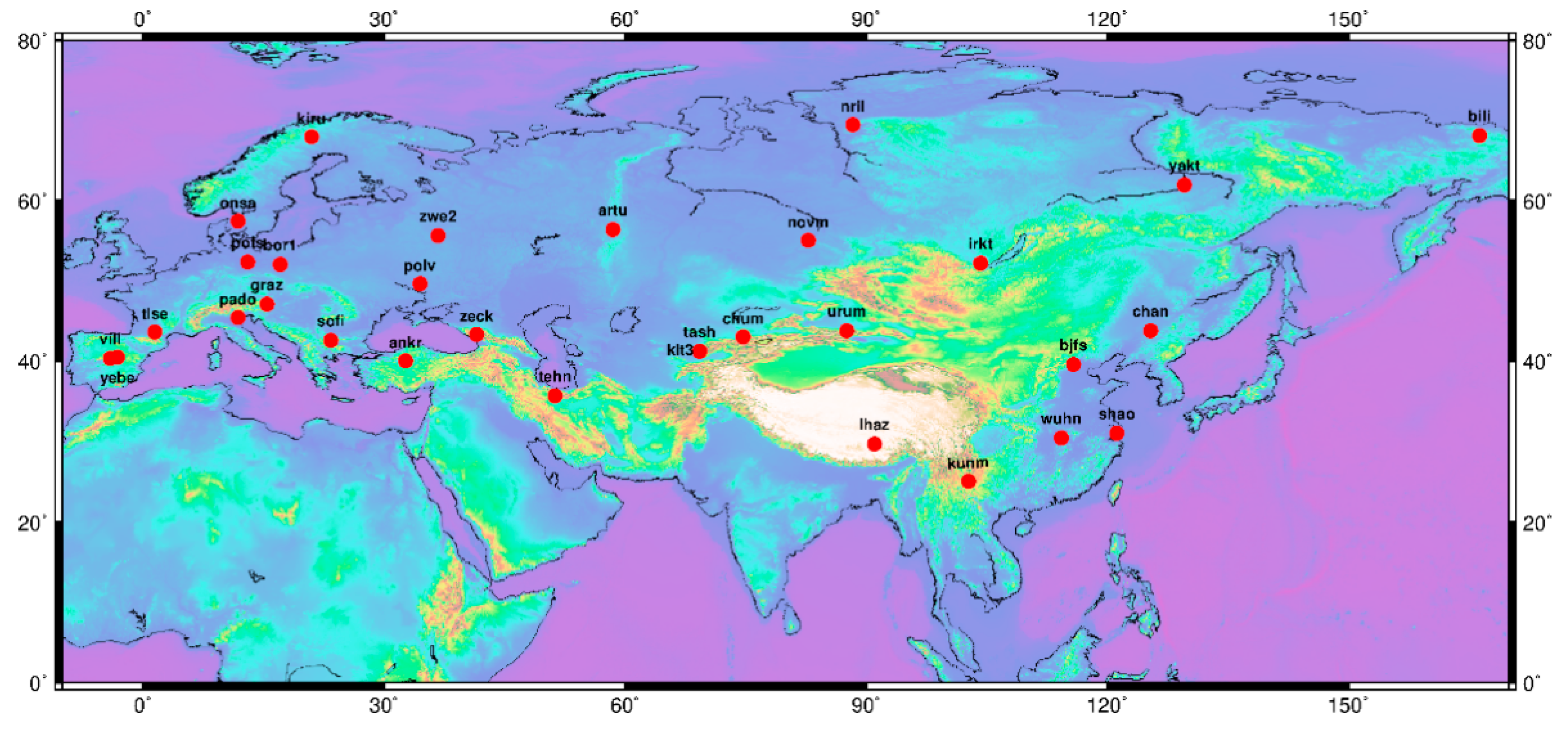
2.1. GPS Data

We used daily GPS data provided by the International Global Navigation Satellite System Service (IGS), which combines the GAMIT (SPOCA) and GIPSY (JPL) solutions. The GAMIT and GIPSY solutions contain the unconstrained geodetic station coordinates, which have been corrected for some geophysical effects (

Table 1. Strategies and geophysical models applied when processing GPS time series with GAMIT and GIPSY.

Geodetic Software	GAMIT/GIPSY
Pole tide	IERS 2003 convention
Earth tides	IERS 2003 convention
Ocean tidal loading	FES04 model
Tropospheric Mapping Function	Global Mapping Function
IGS antenna files	Absolute IGS phase center
General relativity effect	Periodic clock, gravity bending corrections applied
The elevation cut-off angle	10° and 7° for GAMIT and GIPSY, respectively
Data format	24-h observations sampled at 30 s

).

The combined solutions are used so that random processing noise introduced by any individual analysis will be compressed to enhance the signal-to-noise ratio. Fritsche et al. [2] confirmed that the scatter in the vertical component for the combined solutions is smaller by 5–15 mm compared to the scatter in any other analyses. We removed offsets, outliers and the linear trend as described in Nikolaidis in GPS observations [17]. Due to the removal of offsets and outliers as well as other reasons (e.g., the equipment changes or failures), missing data is an inevitable problem in GPS observations. At present, it is difficult to use interpolation methods to calculate the true value due to the complexity of GPS, although the filling of missing data with interpolation will introduce an artificial error. Therefore, GPS site selection is performed using the following criteria. First, the time span of GPS time series should be longer than 2.5 years [18]. Additionally, to minimize the interpolation effect, the number of continuous data gaps should not exceed 15 and the ratio of missing data to entire observations must not be more than 1% for each site [19]. Finally, the selected stations should be uniformly distributed. In this analysis, we filled the data gaps using linear interpolation. It should be noted that the mass loading signal still remains in the GPS observation. Considering that the Eurasian plate is a tectonically stable region and the tectonic noise is minimal, we selected 30 GPS stations located in the Eurasian plate for this analysis from January 2010 to January 2014 (Figure 1).

2.2. Mass Loading

For the non-tidal atmospheric loading deformation, we adopted the provisional product provided by the International Earth Rotation and Reference Systems Service (IERS) Global Geophysical Fluids Center (GGFC)-German Research Centre for Geosciences (GFZ), which is available at http://www.gfz-potsdam.de/en/esmdata. Non-tidal atmospheric mass loads with 0.5° × 0.5° spatial resolution and 6-hourly temporal resolution were estimated by using the surface pressure from the European Centre for Medium-Range Weather Forecasts (ECMWF) operational model [15]. For non-tidal ocean loading deformation, we also adopted the provisional product provided by the GFZ. Non-tidal ocean loads with 0.5° × 0.5° spatial resolution and 6-hourly temporal resolution were derived from non-tidal ocean bottom pressure from the Ocean Model for Circulation and Tides (OMCT) [15]. The GFZ processes the consistent deformation fields from the daily means of the ECMWF atmospheric surface pressure and the OMCT non-tidal ocean bottom pressure to derive the total non-tidal deformation signal. For hydrological loading (HYDL) deformation, we used the provisional product provided by the GFZ. The HYDL with 0.5° × 0.5° spatial resolution and the daily temporal resolution was predicted from the Global Land Surface Discharge Model (LSDM) [20]. The LSDM was found to be composed of the masses of soil moisture, snow and runoff from glaciers, especially water in rivers and lakes. To maintain consistency with GPS heights, the mass loading displacements were all calculated in the center of the figure frame (CF).

2.3. Wavelet Coherence

Firstly, we will briefly outline the continuous wavelet transform (CWT). The CWT of a time series (x_n, n = 1, 2, ..., N) is defined as follows [21]:

$$W_n^x\left(s\right)=\sqrt{\delta t/s}{\displaystyle \sum }_{n^{\prime }=1}^N{x}_{n^{\prime }}{\phi }_0[\left(n^{\prime }-n\right)\frac{\delta t}{s}]$$

(1)

where $W_n^X(s)$ is the wavelet coefficient, $\delta t$ is the time step, s and ${\phi }_0$ are the wavelet scale and the mother function, respectively, and $n\prime$ and $\sqrt{\delta t/s}$ represent the reversed time and the normalization factor, respectively. The idea behind the wavelet transform is to apply the wavelet as a band-pass filter to the time series where the wavelet scale is linearly related to the characteristic period of the filter. Based on the CWT, the WTC of the two-time series X_n and Y_n (n = 1, 2, ..., N) is defined as follows [21]:

$$R_n^2\left(s\right)=\frac{{\left|S\left(s^{-1}{W}_n^{XY}\left(s\right)\right)\right|}^2}{S(s^{-1}|W_n^X\left(s\right){|}^2)·S(s^{-1}|W_n^Y\left(s\right){|}^2)}$$

(2)

where S is the smoothing operator, $W_n^X(s)$ is the wavelet coefficient of the time series X_n, $W_n^Y(s)$ is the wavelet coefficient of the time series Y_n, $W_n^{XY}(s)$ is the cross wavelet transform of the two time series X_n and Y_n, the complex argument arg($W_n^{XY}(s)$) is the local relative phase between X_n and Y_n in time frequency space, s is the wavelet scale, R_n(s) is the localized correlation coefficient and n is the number of stations. The advantage of WTC is its ability to locate regions in the time–frequency domain where the two time series are significantly correlated, and further reveal the relative phase between the two time series in the time–frequency space. In our analysis, the relative phasing of the two time series can be quantified by using the circular mean of the phase or the WTC-based semblance. The definition of the circular mean of a set of angles (α_i, i = 1, 2, ..., N) is expressed as follows [21]:

$$a_m=a\tan 2\left(X,Y\right)=a\tan 2(\frac{1}{n}{\displaystyle \sum }_{i=1}^n\cos ({\alpha }_i),\frac{1}{n}{\displaystyle \sum }_{i=1}^n\sin ({\alpha }_i))$$

(3)

Meanwhile, the WTC-based semblance is defined as follows [22]:

$$\rho =\cos \left({\alpha }_i\right)$$

(4)

The value of ρ ranges from −1 (inversely correlated) to 0 (uncorrelated) to 1 (fully correlated). In this analysis, we used the WTC-based semblance as the key parameter to compare the two time series.

3. Results and Discussion

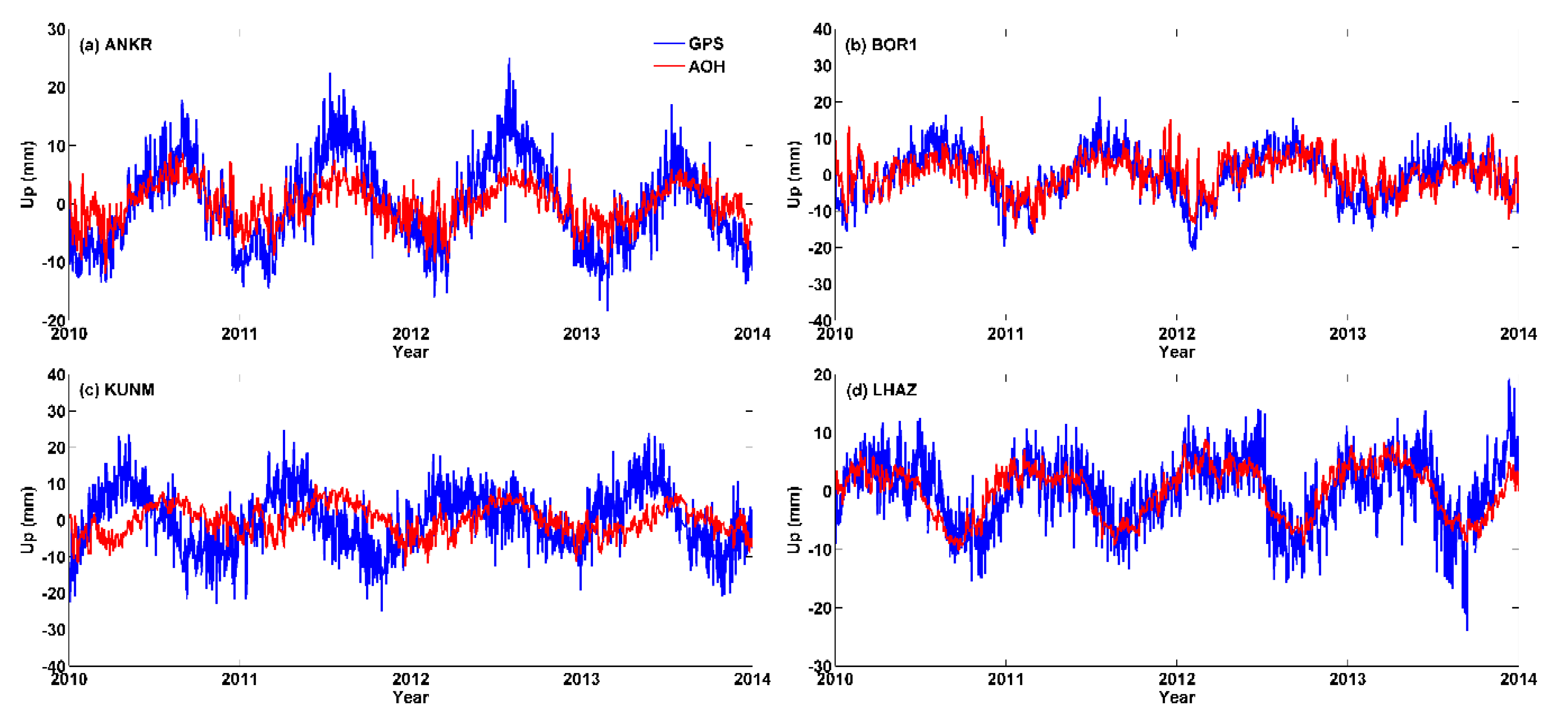
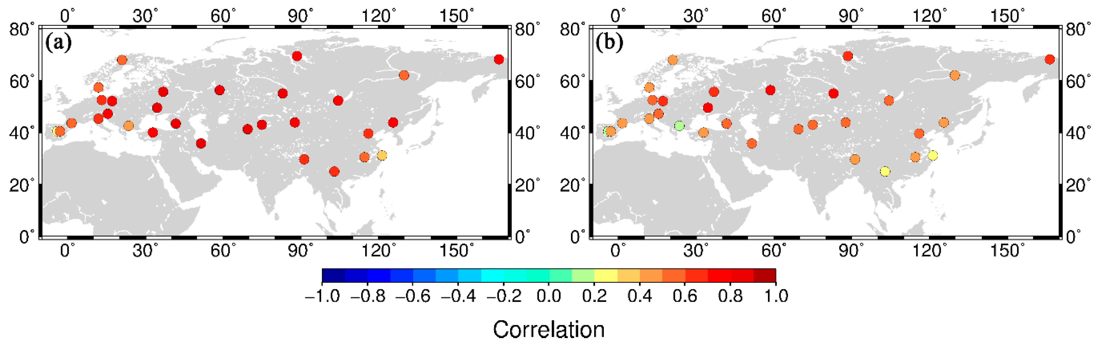
3.1. Root Mean Square Analysis and Correlation Analysis

Given that the mass loading behaves in the vertical direction, we only considered the vertical component in the following analysis.

Figure 2 shows the time series of GPS heights of four stations along with AOH-derived vertical displacements. It is clear from Figure 2 that GPS heights and AOH displacements prominently have an annual variation pattern. AOH displacements track GPS heights well at the ANKR, BOR1 and LHAZ sites, indicating that AOH may be responsible for the non-linear vertical motion of GPS stations. However, for the KUNM site, the AOH deformation signal is not in agreement with GPS height signal due to the phase asynchrony between these two time series.

From

Table 2. The RMS value of GPS height time series and AOH deformation time series respectively.

Site	RMS (GPS)	RMS (AOH)	Site	RMS (GPS)	RMS (AOH)	Site	RMS (GPS)	RMS (AOH)
ANKR	7.6	5.3	KUNM	8.4	6.7	TASH	10.7	7.5
ARTU	11.2	6.1	LHAZ	6.1	4.4	TEHN	6.3	3.9
BILI	8.7	6.2	NOVM	14.5	8.9	TLSE	6.3	5.2
BJFS	8.2	6.2	NRIL	8.6	5.7	URUM	8.4	5.9
BOR1	6.7	4.3	ONSA	6.1	5.1	VILL	8.5	8.3
CHAN	9.3	6.6	PADO	5.8	4.3	WUHN	8.5	7.4
CHUM	9.1	6.0	POLV	9.0	5.2	YAKT	8.4	7.2
GRAZ	7.7	5.6	POTS	8.7	6.6	YEBE	6.3	5.2
IRKT	11.1	8.2	SHAO	6.5	6.3	ZECK	7.9	4.9
KIRU	10.3	8.3	SOFI	10.0	8.9	ZWE2	9.9	6.0

, we can see that the RMS value of GPS height time series varies from 5.8 to 14.5 mm, whereas the RMS value of AOH deformation time series ranges from 3.1 to 7.7 mm. Therefore, AOH cannot fully explain GPS height fluctuations. The Pearson correlation analysis was employed to investigate the correlation between GPS heights and AOH displacements.

As shown in Figure 3a, GPS height and AOH deformation are positively correlated for all the selected sites, while GPS height and AOH deformation have a strong correlation for most sites (correlation coefficient is greater than 0.6). The strong correlation between GPS heights and AOH displacements may be attributed to the significantly related annual signal. Apart from the annual component, the other components in AOH deformation may act as the potential candidates for determining the strong correlation between GPS heights and AOH displacements. Therefore, by adopting the least squares method, the annual term was removed from GPS heights and AOH displacements to generate GPS height residuals and AOH deformation residuals, respectively. Figure 3b presents the correlation coefficients between GPS height residuals and AOH deformation residuals. All the selected sites are positively correlated, and most sites have a medium correlation (correlation coefficient is between 0.4 and 0.6). Therefore, the correlation between GPS height and AOH deformation is reduced after removing the annual signal.

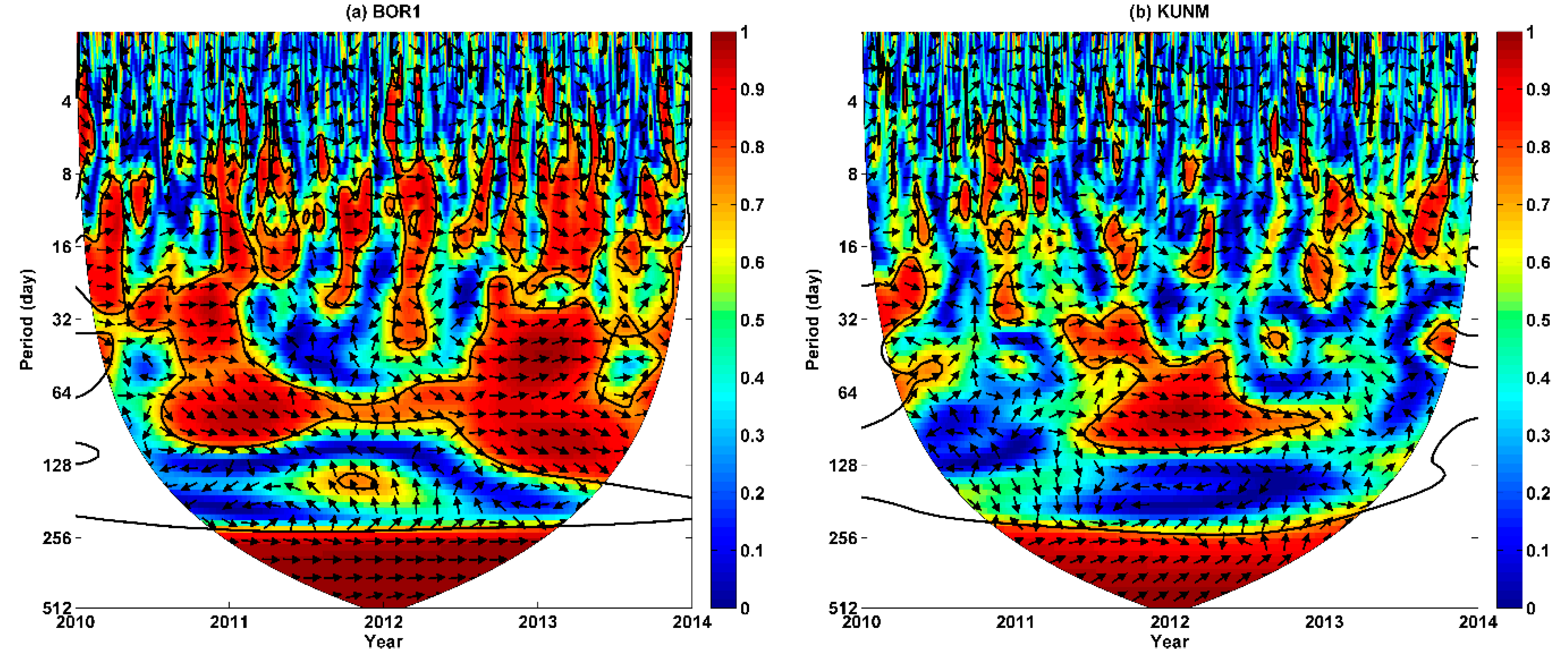
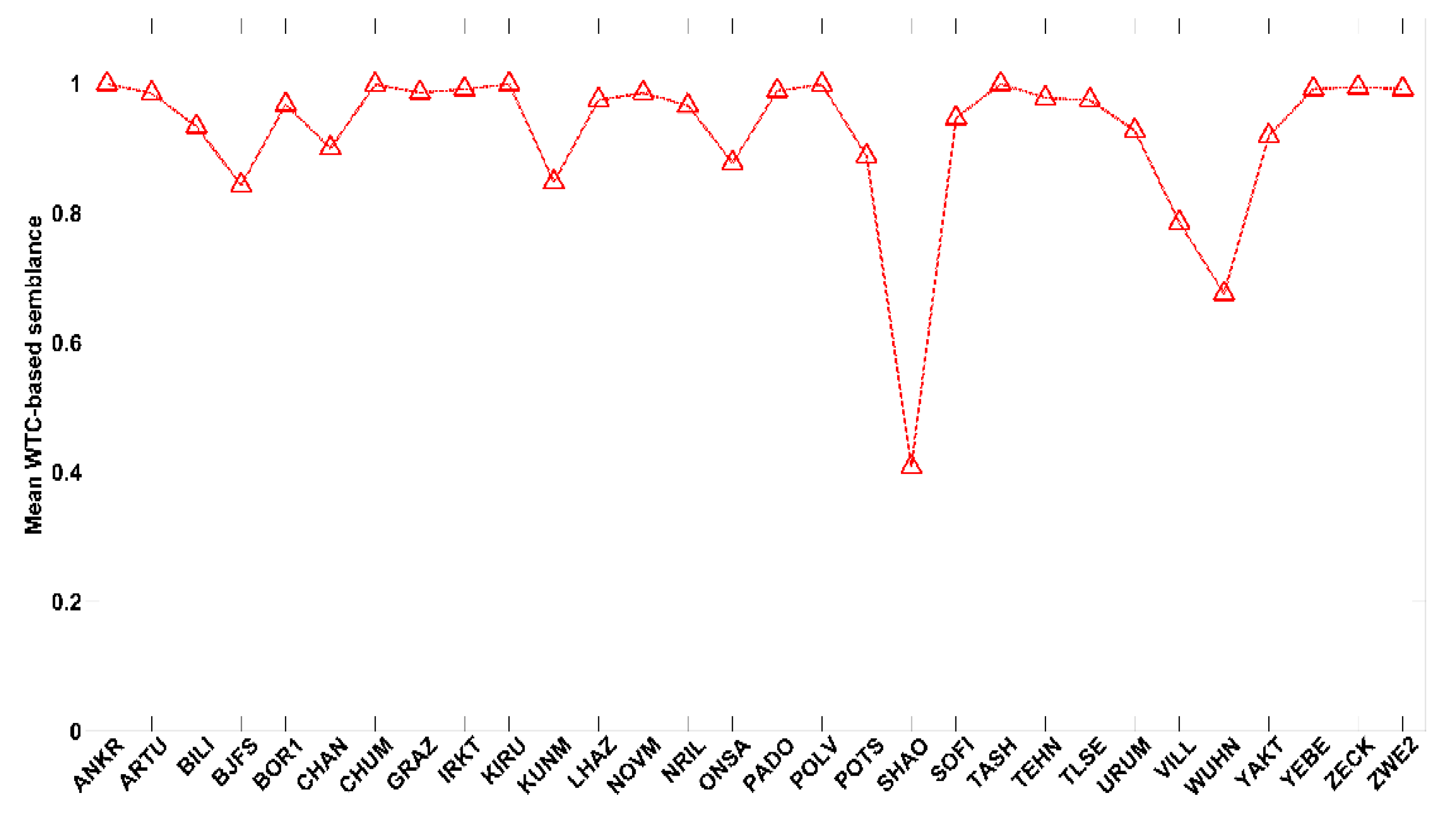
3.2. Wavelet Coherence Analysis

Considering that the Pearson correlation analysis is aimed to simply find a correlation in the time domain, there are several issues in determining the specific relationship between GPS heights and AOH displacements with this analysis. Firstly, since the annual component plays an essential role, a more detailed insight aimed at the annual scale (frequency) should be considered. Secondly, in addition to the annual component, other components may potentially be relevant. Lastly, the relationship (e.g., correlation coefficient and relative phase) may change over time. Here, we propose to employ the WTC to overcome all the above-mentioned issues.

The WTC spectrum of GPS height time series and AOH deformation time series for the BOR1 site and KUNM site are shown in Figure 4. The reason that we chose these two stations is that Figure 1 displays the approximate relative phase between GPS heights and AOH displacements for the BOR1 site and KUNM site, which can be used to validate the results of WTC. The thick contour indicates the 95% confidence interval against the red noise, while the phase of the area within the cone of influence was unaccounted for due to the edge effects. The relative phasing relationship is denoted by arrows (with in-phase pointing right, anti-phase pointing left and GPS height leading AOH deformation to 90° pointing straight down). Figure 4 shows that the correlation between these two time series is considerably high at a frequency that is closest to 1 cycle per year (cpy). From Figure 4a, we can see that GPS height time series and AOH deformation time series are in phase at the period closest to 1 year for the BOR1 site, indicating that AOH is responsible for the annual fluctuation in GPS heights. From Figure 4b, we can see that GPS height time series and AOH deformation time series are not in phase at the period closest to 1 year for the KUNM site, indicating that AOH is not responsible for the annual fluctuation in GPS heights. For the high-frequency components (in the period band of fewer than 256 days), although a locally significant correlation was detected, the relative phase angles of the high-frequency components fluctuated sharply, indicating that the GPS height signal and AOH deformation signal are not in phase. Consequently, it is demonstrated that the geophysical effects cannot explain the sub-seasonal oscillations in GPS observations [23].

Since the fluctuation range of the time-variable relative phasing at the period closest to 1 year is small, the mean WTC-based semblance was computed to quantitatively express the relative phase between these two signals. Following the same method as depicted in Figure 4, the WTC was used to analyze the relative phase between GPS height time series and AOH deformation time series for the other sites, with the mean WTC-based semblance at the frequency closest to 1 cpy.

As shown in Figure 5, the average value of the WTC-based semblance for most, but not all, sites are close to 1, indicating that AOH is not a complete representation of the driving force for the non-linear GPS site motion. From Figure 5, we can see that for the SHAO site, the mean semblance is only 0.4, while the other 10 sites (NILI, BJFS, CHAN, KUNM, ONSA, POTS, SOFI, URUM, VILL and WUHN) have a mean semblance value that is close to 0.7–0.9. Other geophysical effects (e.g., groundwater), GPS systematic errors (e.g., inaccurate local multi-path and tropospheric modelling) and AOH modelling errors (e.g., interpolation method) can lead to the phase asynchrony between GPS observations and mass loading displacements. A measure of RMS reduction ratio expressed in percent (ΔRMS%) is employed to quantify the correction performance of AOH models:

$$\Delta \mathrm{RMS}\%=\frac{\mathrm{RMS}\left(\mathrm{GPS}\right)-\mathrm{RMS}(\mathrm{GPS}-\mathrm{AOH})}{\mathrm{RMS}\left(\mathrm{GPS}\right)}$$

(5)

Table 3. The RMS reduction ratio in percent when correcting GPS heights with AOH displacements.

Site	ΔRMS%	Site	ΔRMS%	Site	ΔRMS%
ANKR	30.2%	KUNM	20.1%	TASH	30.2%
ARTU	45.3%	LHAZ	27.3%	TEHN	38.0%
BILI	28.8%	NOVM	38.7%	TLSE	18.0%
BJFS	23.7%	NRIL	34.2%	URUM	29.7%
BOR1	35.6%	ONSA	17.1%	VILL	3.0%
CHAN	28.4%	PADO	25.7%	WUHN	9.0%
CHUM	33.9%	POLV	42.6%	YAKT	14.6%
GRAZ	27.6%	POTS	24.1%	YEBE	18.1%
IRKT	26.2%	SHAO	4.2%	ZECK	38.3%
KIRU	18.9%	SOFI	14.0%	ZWE2	39.6%

indicates that all sites experience a reduction in their RMS values when corrected by AOH, revealing the feasibility of correcting GPS height with the mass loading model. From Table 3, we can see that a relatively poor improvement occurs at the SHAO, VILL and WUHN sites, where there is a significant phase asynchrony between GPS heights and AOH displacements.

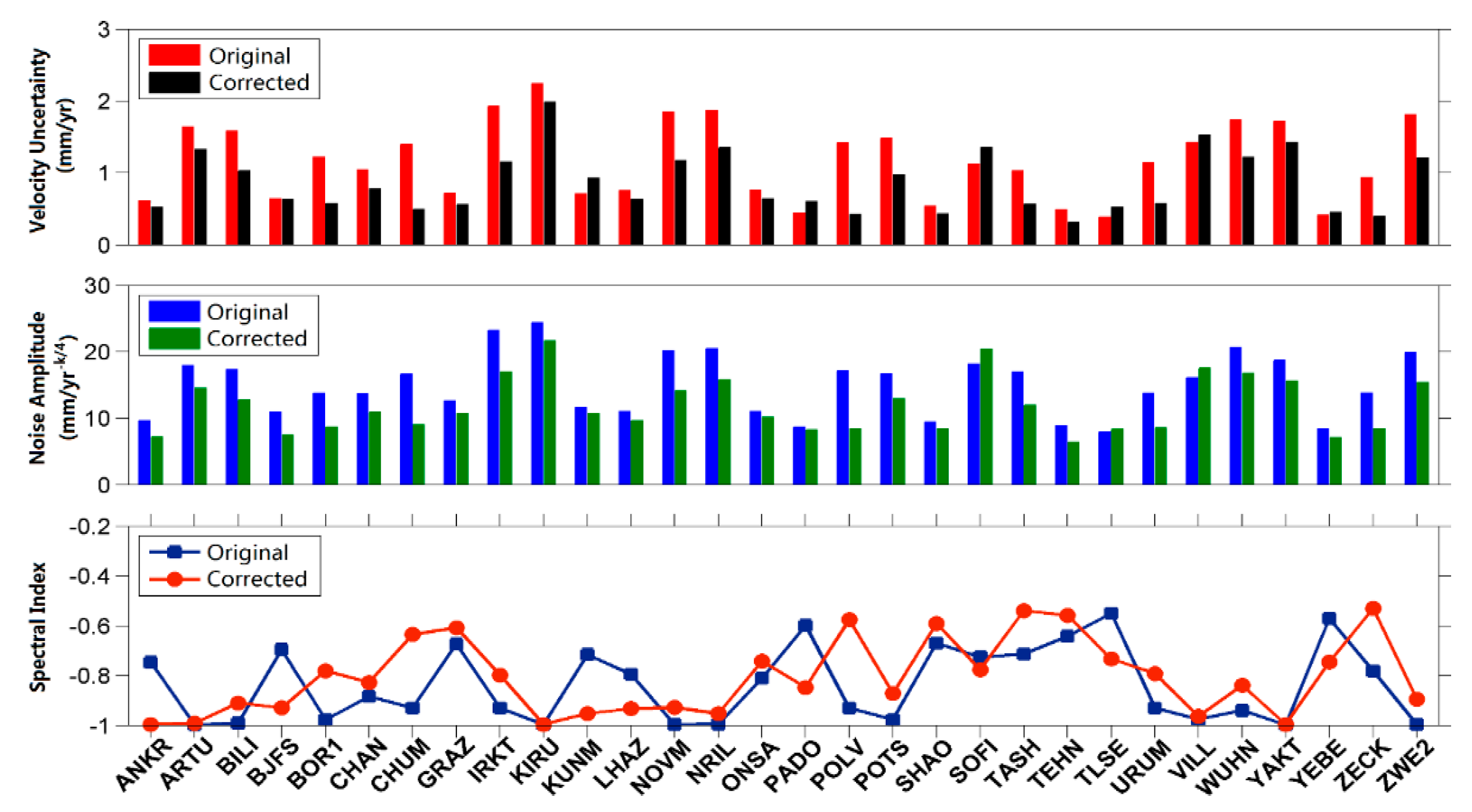
3.3. Noise and Velocity Analysis

Errors in the mass loading model are currently difficult to quantify. Nonetheless, they will certainly enter into our estimates of surface deformation [24]. In this case, aside from investigating the RMS reduction of GPS position time series, discussing the effect of mass loading corrections on the velocity and noise estimates is equally important. In this study, we adopted the Hector software to determine the velocity and its uncertainty with pre-assumed power-law noise and white noise [25]. The software can sufficiently describe the stochastic properties of most daily GPS position time series. The noise parameters, including the spectral indices and noise amplitudes, were also estimated before and after the AOH corrections by using the maximum likelihood estimation to analyze the change in noise properties. The accuracy of velocity is calculated based on the following formula [26]:

$$m_v\approx \pm \sqrt{\frac{A_{PL}^2·\mathsf{\Gamma }\left(3-K\right)·\mathsf{\Gamma }\left(4-K\right)·{\left(N-1\right)}^{K-3}}{\Delta T^{2-\frac{K}{2}}·{\left[\mathsf{\Gamma }\left(2-\frac{K}{2}\right)\right]}^2}}$$

(6)

where m_v is the accuracy of velocity, A_PL is the amplitude of noise, K is the spectral index, Γ is the gamma function, N is the number of data in the time series and ΔT is the sampling interval.

The middle histogram in Figure 6 demonstrates that the power-law noise amplitude is mostly decreased when AOH corrections are applied. The small amplitude of noise after AOH corrections indicates the small scatter of residuals, and consequently a considerably stable solution for the determination of site velocity. Meanwhile, the bottom histogram in Figure 6 indicates that the spectral index shifts from a flicker noise (k = −1) to white noise (k = 0) in most sites. Hence, the loading signals may be superimposed on the stochastic process realization. The removal of AOH deformation for GPS stations causes a reduction in median velocity error from 1.17 to 0.87 mm/year in median power-law noise amplitude from 14.99 to 11.84 mm/year-k/4 and in the median spectral index from −0.84 to −0.81 mm/year-k/4. The results indicate that AOH corrections altered the noise properties of GPS height time series. Based on Equation (6), changes in the noise properties will certainly influence the estimates of velocity uncertainties. Accordingly, AOH corrections will potentially affect the velocity-field determination, and thus, its geodynamical interpretation. From the top histogram in Figure 6, we can see that for 24 out of the 30 sites the velocity uncertainty estimates decrease after AOH corrections. However, for 6 out of the 30 sites (KUNM, PADO, SOFI, TLSE, VILL and YEBE) the velocity uncertainty increases due to the increased amplitude of noise and/or the decreased spectral index after AOH corrections. This indicates that errors or noises are introduced when implementing the mass loading correction, suggesting that the correction of GPS heights with the mass loading model is potentially feasible but not sufficient.

4. Conclusions

Considering the limitations of the RMS analysis—i.e., that it can only be used in the time domain—in this paper, WTC was applied to identify the correlation and relative phases between GPS height time series and AOH deformation time series in the time–frequency space. The results of the WTC-based semblance analysis indicate that AOH is not a complete representation of the driving force for the non-linear GPS site motions. AOH modelling errors (e.g., interpolation method), other geophysical effects (e.g., groundwater) and GPS system errors (e.g., local multi-path and tropospheric mis-modelling) can cause the phase asynchrony between GPS observations and AOH displacements. Furthermore, the impact of AOH corrections on noise estimates were investigated. The results showed that, for most sites, the velocity uncertainty is improved after AOH corrections, whereas the velocity uncertainty increases for some sites due to the large amplitude of noise and/or the decreased spectral index after AOH corrections. Overall, this indicates that the posterior mass loading model correction is potentially feasible but not sufficient. In conclusion, the wavelet coherence analysis is a useful exploratory tool to identify correlated behaviors and the time-variable relative phases between GPS observations and mass loading displacements.

References

1. Williams, S.D.P.; Penna, N.T. Non-tidal ocean loading effects on geodetic GPS heights. Geophys. Res. Lett. 2011, 38, 159–164. [Google Scholar] [CrossRef]
2. Fritsche, M.; Döll, P.; Dietrich, R. Global-scale validation of model-based load deformation of the Earth’s crust from continental watermass and atmospheric pressure variations using GPS. J. Geodyn. 2012, 59–60, 133–142. [Google Scholar] [CrossRef]
3. Chanard, K.; Avouac, J.P.; Ramillien, G.; Genrich, J. Modeling deformation induced by seasonal variations of continental water in the Himalaya region: Sensitivity to Earth elastic structure. J. Geophys. Res. Solid Earth 2014, 119, 5097–5113. [Google Scholar] [CrossRef] [Green Version]
4. Braitenberg, C. The deforming and rotating Earth-A review of the 18th International Symposium on Geodynamics and Earth Tide, Trieste 2016. Geod. Geodyn. 2018, 9, 187–196. [Google Scholar] [CrossRef]
5. Marcin, R.; Tomasz, L. Analysis of seasonal position variation for selected GNSS sites in Poland using loading modelling and GRACE data. Geod. Geodyn. 2017, 8, 253–259. [Google Scholar]
6. Dach, R.; Dietrich, R. Influence of the ocean loading effect on GPS derived precipitable water vapor. Geophys. Res. Lett. 2000, 27, 2953–2956. [Google Scholar] [CrossRef] [Green Version]
7. Blewitt, G. Self-consistency in reference frames, geocenter definition, and surface loading of the solid Earth. J. Geophys. Res. Solid Earth 2003, 108, 2103. [Google Scholar] [CrossRef]
8. Davis, J.L.; Elósegui, P.; Mitrovica, J.X.; Tamisiea, M.E. Climate-driven deformation of the solid Earth from GRACE and GPS. Geophys. Res. Lett. 2004, 31, 1–4. [Google Scholar] [CrossRef]
9. Ouellette, K.J.; De-Linage, C.; Famiglietti, J.S. Estimating snow water equivalent from GPS vertical site-position observations in the western United States. Water Resour. Res. 2013, 49, 2508–2518. [Google Scholar] [CrossRef] [PubMed] [Green Version]
10. Chew, C.C.; Small, E.E. Terrestrial water storage response to the 2012 drought estimated from GPS vertical position anomalies. Geophys. Res. Lett. 2014, 41, 6145–6151. [Google Scholar] [CrossRef] [Green Version]
11. Amos, C.B.; Audet, P.; Hammond, W.C.; Burgmann, R.; Johanson, I.A.; Blewitt, G. Uplift and seismicity driven groundwater depletion in central California. Nature 2014, 509, 483–486. [Google Scholar] [CrossRef] [PubMed]
12. Fu, Y.; Freymueller, J.T. Seasonal and long-term vertical deformation in the Nepal Himalaya constrained by GPS and GRACE measurements. J. Geophys. Res. 2012, 117, B03407. [Google Scholar] [CrossRef]
13. Fu, Y.; Argus, D.F.; Freymueller, J.T.; Heflin, M.B. Horizontal motion in elastic response to seasonal loading of rain water in the Amazon Basin and monsoon water in Southeast Asia observed by GPS and inferred from GRACE. Geophys. Res. Lett. 2013, 40, 6048–6053. [Google Scholar] [CrossRef] [Green Version]
14. Van-Dam, T.; Wahr, J.; Lavallée, D. A comparison of annual vertical crustal displacements from GPS and Gravity Recovery and Climate Experiment (GRACE) over Europe. J. Geophys. Res. 2007, 112, B03404. [Google Scholar] [CrossRef]
15. Dill, R.; Dobslaw, H. Numerical simulations of global-scale high-resolution hydrological crustal deformations. J. Geophys. Res. Solid Earth 2013, 118, 5008–5017. [Google Scholar] [CrossRef] [Green Version]
16. Jiang, W.; Li, Z.; Van-Dam, T.; Ding, W. Comparative analysis of different environmental loading methods and their impacts on the GPS height time series. J. Geod. 2013, 87, 687–703. [Google Scholar] [CrossRef]
17. Nikolaidis, R. Observation of Geodetic and Seismic Deformation with the Global Positioning System; University of California San Diego: San Diego, CA, USA, 2002. [Google Scholar]
18. Blewitt, G.; Lavallee, D. Effect of annual signals on geodetic velocity. J. Geophys. Res. 2002, 107, 2145. [Google Scholar] [CrossRef]
19. Li, Z.; Yue, J.P.; Li, W.; Lu, D.K. Investigating mass loading contributes of annual GPS observations for the Eurasian plate. J. Geodyn. 2017, 111, 43–49. [Google Scholar] [CrossRef]
20. Dill, R. Hydological Model LSDM for Operational Earth Rotation and Gravity Field Variations; Scientific Technical Report STR08/09; GFZ Potsdam: Potsdam, Germany, 2008. [Google Scholar]
21. Grinsted, A.; Moore, J.C.; Jevrejeva, S. Application of the cross wavelet transform and wavelet coherence to geophysical time series. Nonlinear Process. Geophys. 2004, 11, 561–566. [Google Scholar] [CrossRef] [Green Version]
22. Cooper, G.; Cowan, D. Comparing time series using wavelet-based semblance analysis. Comput. Geosci. 2008, 34, 95–102. [Google Scholar] [CrossRef]
23. Ray, J.; Griffiths, J.; Collilieux, X.; Rebischung, P. Subseasonal GNSS positioning errors. Geophys. Res. Lett. 2013, 40, 5854–5860. [Google Scholar] [CrossRef] [Green Version]
24. He, X.; Jean-Philippe, M.; Hua, X.; Yu, K.; Jiang, W.; Zhou, F. Noise analysis for environmental loading effect on GPS time series. Acta Geodyn. Geomater. 2017, 185, 131–142. [Google Scholar] [CrossRef]
25. Xu, C.; Yue, D. Monte Carlo SSA to detect time-variable seasonal oscillations from GPS-derived site position time series. Tectonophysics 2015, 665, 118–126. [Google Scholar] [CrossRef]
26. Bos, M.; Fernandes, R.; Williams, S.; Bastos, L. Fast error analysis of continuous GNSS observations with missing data. J. Geod. 2013, 87, 351–360. [Google Scholar] [CrossRef]
Figure 1. Spatial distribution of the 30 GPS stations used in this study.
Applsci 08 01851 g001
Figure 2. GPS height time series (blue) and atmospheric, oceanic and hydrological loading (AOH) deformation time series (pink) for (a) Ankara, Turkey (ANKR); (b) Borowiec, Poland (BOR1); (c) Kunming, China (KUNM); and (d) Lhasa, China (LHAZ).
Applsci 08 01851 g002
Figure 3. (a) Correlation between the GPS height and the AOH deformation; (b) Correlation between the GPS height residuals and AOH deformation residuals.
Applsci 08 01851 g003
Figure 4. The wavelet coherence (WTC) spectrum of GPS heights and AOH displacements for (a) BOR1 site and (b) KUNM site.
Applsci 08 01851 g004
Figure 5. Mean value of the WTC-based semblance at the period closest to 1 year for 30 sites.
Applsci 08 01851 g005
Figure 6. Comparison of the velocity uncertainty and noise parameters before and after AOH corrections.
Applsci 08 01851 g006