Methodology for Existing Railway Reconstruction with Constrained Optimization Based on Point Cloud Data

Abstract

The reconstruction of an existing railway is important for railway reformation or double-track design. Obtaining the curve parameters of the railway and the location of the main stake accurately and rapidly is the key issue for existing railway reconstruction. A new method based on point cloud data is proposed in this paper. The issue of reconstruction was transformed into an optimization problem by constructing the objective function and introducing the constraint. With consideration of the slope of the curves’ chord, the robust local weighted moving average method was used for de-noising. The time complexity was reduced greatly after separating the curve unit. The proposed method can obtain the coordinates of the main stake and the parameters of the railway by particle swarm optimization using a full direction search, combining the design requirements and geometric relations of the railway. Finally, some experiments on the design data and measured data were conducted to verify the validity of the proposed method. The results also show that the proposed method is very effective and useful for existing railway reconstruction.

1. Introduction

By the end of 2017, the operation length of China’s railways exceeded 127,000 km, including 25,000 km of high-speed railway. The maintenance and transformation of existing railway is necessary to ensure the efficiency and safety of railway operations [1]. Due to the effects of wheels and rails, ballast settlement, environmental change, and so forth, the railway is inevitably offset from the designed state after a period of operation. Railway reconstruction refers to recovering the railway to as close to the delivery status as possible based on the original design data and measured data. Meanwhile, using the results of railway reconstruction as a reference standard is an important aspect for the transformation of the existing railway and design of the new double-track railway [2]. The accuracy and quality of the reconstruction influence the time limit, cost, and safety of the engineering.

Existing railway reconstruction is an important research topic in the fields of railway engineering [3], surveying and mapping engineering [4], reverse engineering [5], and computing science [6]. In recent years, scientists have conducted extensive investigations in the field of existing railway reconstruction based on the coordinate method. Ding et al. reconstructed an existing railway using the robust least squares method after each feature point was identified [7]. When the arc-diameter ratio is small, the circle parameters obtained by fitting are not accurate. Li et al. used the complex Simpson’s Equation based on the curvature change of the centerline to develop the calculation method suitable for various line types [8]. Once the measurement error or measurement interval is large, curvature change would be too disordered to identify feature points. In 2009, Li and Pu proposed a plane reconstruction algorithm that solved the minimal value of the function and corresponding three arguments using a direction acceleration method, and discussed how to determine the initial values and constraints from the design code [9]. However, the method of manually identifying the feature points cannot reach the actual requirements. At the same time as the development of the swarm intelligence algorithm, there was also the genetic algorithm (GA), ant colony algorithm (ACA), and particle swarm optimization (PSO) study on existing railway reconstruction [10]. Xu et al. developed a GA that optimized the evaluation function by selection, crossover, and mutation operators based on the initial values calculated by a feasible region [11]. Yang introduced the ACA into the existing railway reconstruction of the plane and longitudinal section [12]. Curve radius, transition curve length, and curve length were included as parameters in the model, and the optimization results that met the various constraints were calculated. Miao presented a railway reconstruction method based on the PSO algorithm which calculated the reconstruction parameters in the shift distance calculation involving the limitation of the control point and the requirement for integer parameters. This method could calculate the curve parameters of multiple existing railway units [13].

The premise of railway reconstruction is to obtain the location and status of the track. Therefore, it is necessary to resurvey the railway. Various involute-based, coordinate-based, and even point cloud data-based methods have been widely conducted worldwide to actively promote its relevant applications. For example, the string lining method is applied to existing railway curve realignment [14]. The deflection method and coordinate method can achieve a higher precision compared to the former method [15]. Currently, the involute-based method has been gradually phased out in actual engineering because of the long track lining distance [16]. The coordinate-based method, which has the characteristics of less disturbance and improved safety, is popular in practical work. Obtaining the 3D coordinates of the railway is the main aim of the coordinate method [17]. In the method of total station free-stationing, measuring the plane position and the rail’s top elevation of the track centerline can achieve accurate results using the total station and level [18]. However, there are two problems with the free-stationing method of the total station. First, it is difficult to accurately find the steel centerline, which was measured with a steel ruler or a gauge. This method was time-consuming, laborious, and low in measurement accuracy. Second, the total station must be placed within the visible range during the entire measurement. It is essential to set a lot of transfer points where the measuring track does not have visibility or has no proper place for a measuring prism. Hence, the method of total station free-stationing is suitable for a single curve, but not for an entire continuous railway containing multiple curve units. Ding successfully applied real-time kinematic (RTK), which is a global navigation satellite system (GNSS) carrier phase measurement technology, to an existing railway resurvey with high efficiency and high accuracy [19]. The above two problems existing in total station free-stationing still cannot be ignored.

Whether using the involute-based method or coordinate-based measurement, working on the railway is inevitable. With the enhancement of the railway running speed and enlarging of traffic density, the “skylight” operation time is too short for a survey, which creates the need for a noncontact measuring method. Traditional methods including the string lining method, the deflection method, the free-stationing method, and RTK face great challenges that are unsuitable for the gradual development trend of high-speed railways. At present, due to speed, safety, and low cost, three-dimensional laser scanning technology has been applied effectively to solve these problems. In particular, point cloud data can provide detailed information in track detection and support railway reconstruction. Scholars have done a lot of research on using measurement scheme design, point cloud data processing, and feature extraction to develop a reconstruction model. Zhu and Hyyppa [20] proposed a method that reconstructed an entire railway environment successfully from point cloud datasets. However, the goal was to produce a final visualization of railway environments, and rail roads were considered part of the ground. Yang and Fang [21] presented an automated method to detect roads from mobile laser scanning (MLS) point cloud data. Both the geometry and intensity data of railway roads were utilized to extract track points and to model roads. Anita et al. [22] compared the quality of the scans from a phase-based scanner and a hybrid time-of-flight scanner by fitting different sections of the track profile to its matching standardized rail model. However, both scanners were so sensitive to noise and artefacts that the proposed method was not robust. Liu et al. [23] proposed a new approach that uses terrestrial laser scanning (TLS) to detect subsidence and irregularities in a track by fitting boundaries of the cross section of the track. The results indicated that the subsidence difference between TLS and precise leveling was 2 to 3 mm and the difference in the geometric parameters of the tracks was 1 to 2 mm. The approach, however, is not automated. Elberinka et al. [24] fitted a parametric model of a rail piece to the points along each track and estimated the position and orientation parameters of each piece’s model. This method is not suitable for highly detailed measurements with millimeter precision. Moreover, when reconstructing a complex railway environment, the complexity is based on the diversity of the objects of the railroad infrastructure and surroundings, which include railroads, buildings, power lines, pylons, street/traffic lights, and so forth. The fusion of light detection and ranging (LiDAR) data and images can achieve good results [25]. In this study, from the theoretical perspective, the interpretation, the general mathematical descriptions, and the considerations for some special constraint conditions are presented. Then, four experiments to prove the feasibility, suitability, robustness, and practicality of the proposed method from design data, measurement data, and artificial data were introduced, respectively. Thus, this study provides implications for the research and business applications of existing railway reconstruction based on point cloud data.

2. Materials and Methods

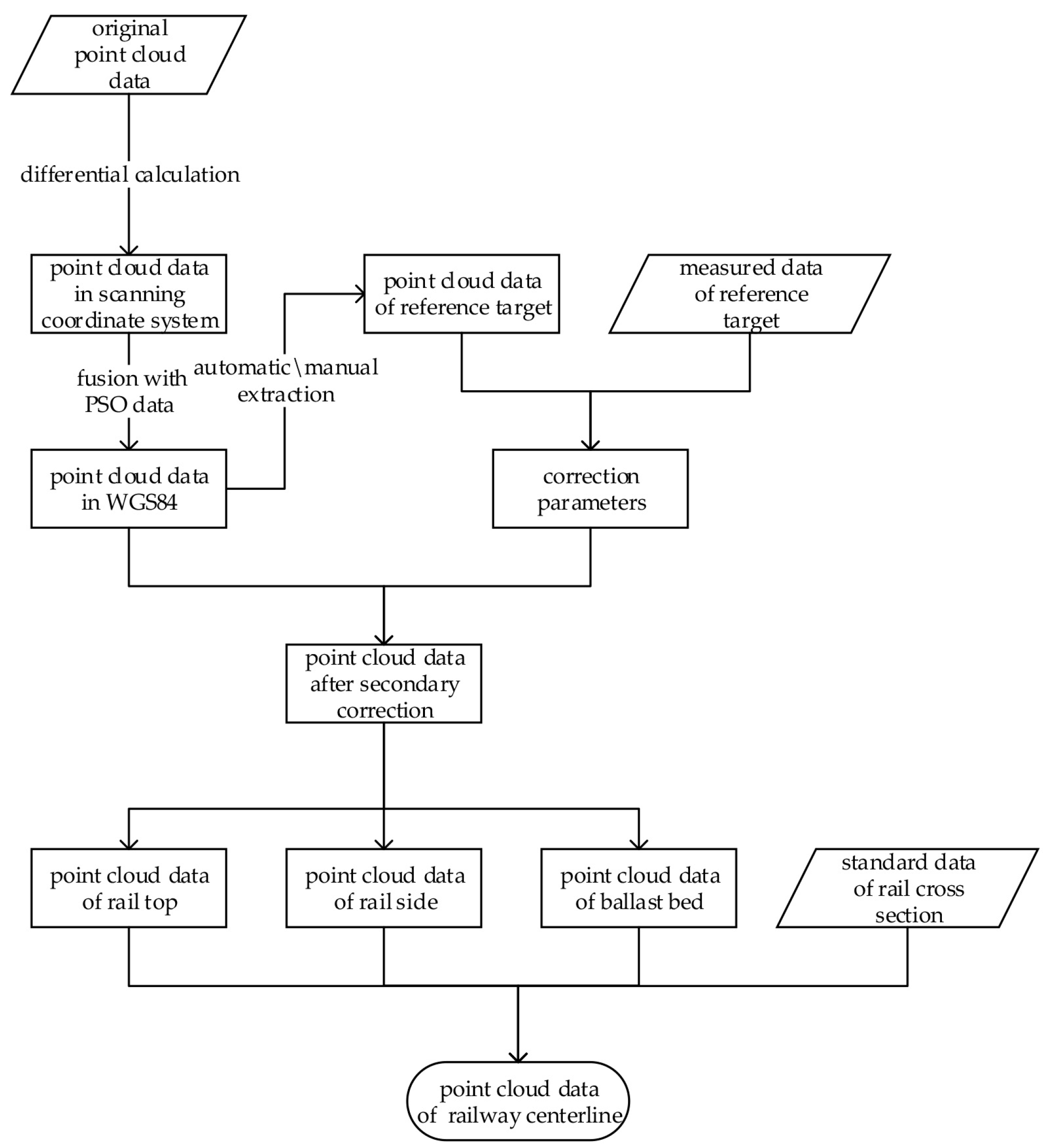
The research method in this paper is based on railway centerline point cloud data, so it is essential to extract high-quality centerline data from the original vehicle-borne laser 3D scanning point cloud data. The difference calculation of inertial navigation system (INS)/GNSS data was used to obtain accurate train trajectory and attitude, and the point cloud data in the scanner coordinate system was fused with the processed position orientation system (POS) data to obtain the point cloud data in the WGS84 coordinate system. In order to ensure the accuracy, the error generated in the point cloud data acquisition solution and processing with measured target point data was corrected. In the MicroStation software, point cloud data was classified into rail top data and rail side data by pulling the section along the track direction and moving the cross section based on the standard data of the rail. Railway centerline data is obtained by “panning” the rail top and rail side point cloud data. The flowchart for rail centerline extraction is shown in Figure 1.

2.1. Objective Function

In order to describe the railway reconstruction problem, the sum of squares for the track lining distance is used as the evaluation index. That is:

$$F={\displaystyle \sum _{i=1}^n{\left|{\Delta }_i\right|}^2}$$

(1)

where $n$ and $\left|{\Delta }_i\right|$ are the number of the measuring point and track lining distance of measuring point i, respectively, and $F$ is the evaluation function. The smaller the $F$ value is, the higher reconstruction accuracy is. Therefore, the railway reconstruction was presented as an optimization problem. Then, the objective function ($Q$) can be calculated from the minimization of the sum of squares for track lining the distance of the measuring point.

$$Q=MIN({\displaystyle \sum _{i=1}^n{\left|{\Delta }_i\right|}^2})$$

(2)

The reconstruction of the existing railway includes two parts: plane reconstruction and longitudinal profile reconstruction. Plane reconstruction is the basis of longitudinal reconstruction, and longitudinal profile reconstruction must be done after plane reconstruction. In addition, because the transition curve exists in in the track plane, the reconstruction of plane reconstruction is more difficult than longitudinal reconstruction. Therefore, this paper focuses on the method of existing railway plane reconstruction. The multiple linear planes were constituted by fundamental railway plane geometry elements, i.e., straight lines, circular curves, and transition curves. In general, the basic curve unit of a typical rail plane is made up of a “straight line–transition curve–circular curve–transition curve–straight line” sequence [26], as shown in Figure 2. In the basic curve unit reconstruction model, it is only necessary to obtain the radius of the circle curve and the first and second transition curve to determine the position of the line plane after the first and second intermediate straight lines are confirmed. As the premise of the existing railway reconstruction, an intermediate straight line will directly affect reconstruction accuracy. In a continuous rail plane curve reconstruction model (containing multiple basic curve units), an intermediate straight line is a parameter factor in the existing railway reconstruction model.

In the method of total station free-stationing, after the curve-independent coordinate system is established, two points which are rather far away on the straight section are selected to determine the intermediate straight line, or multiple measuring points are selected based on the least squares method. However, when the straight line segment is short or the straight line segment is difficult to determine, this method results in a large error. Moreover, it is difficult to accurately find ZH and HZ from point cloud data, and the track lining distance of the measuring point is also difficult to find directly after existing railway reconstruction. In order to solve the above problems, the sum of the squares for the distance from the point cloud data to the reconstructed track is used as an evaluation parameter in this article, and the segmentation feature of the intermediate straight line is also an important factor. In the straight-line segment, the distance from the point to the straight line is solved using Equation (3). In the segment of the circular curve, the distance can be calculated from the difference between the distance from the center of the circle to the radius (Equation (4)). The common line type of transition curves in China’s railways is a cubic parabola, for which it is not easy to find the close form to calculate the distance from the point to the transition curve. Thus, this paper obtains the track lining distance by an iterative method.

$$d_{\mathrm{line}}=\frac{k{x}_i-y_i+b}{\sqrt{1+k^2}}$$

(3)

$$d_{circle}=\left|R-\sqrt{{(x_i-x_{\mathrm{o}})}^2+{(y_i-y_{\mathrm{o}})}^2}\right|$$

(4)

where $k$ and $b$ are the slope and intercept respectively, and $(x_i,y_i)$ is the coordinate of measuring point $i$. $R$ and $(x_{\mathrm{o}},y_{\mathrm{o}})$ are circular curves corresponding to circle radius and the center $O$ coordinate. $d_{\mathrm{zh}}$ and $d_{\mathrm{hz}}$ express the distance from the point cloud data to the first and second intermediate straight line, and $d_{\mathrm{hy}}$, $d_{\mathrm{yh}}$ stand for the distance from point cloud data to the first and second transition curve. $d_{\mathrm{yy}}$ is the distance from the point cloud data to the circular curve. Then, the track lining distance between the measuring point to the reconstructed railway is the shortest distance from the point cloud data to the five line elements, as is shown in Equation (4).

$$D=MIN(d_{\mathrm{zh}},d_{\mathrm{hz}},d_{\mathrm{hy}},d_{\mathrm{yh}},d_{\mathrm{yy}})$$

(5)

Based on Equations (3)–(5), it is not difficult to find that the optimizing model is closely related to the circle curve radius $R$; the circle center $O$; the first and second intermediate straight line slope, $k_1$ and, $k_2$;and intercepts $b_1$ and $b_2$; and the first and second transition curves $l_1$ and $l_2$. Thus, the distance function $D(R,O,k_1,k_2,b_1,b_2,l_1,l_2)$ is established for $R,O,k_1,k_2,b_1,b_2,l_1,l_2$.

Suppose: $\mathbf{X}={(R,O,k_1,k_2,b_1,b_2,l_1,l_2)}^T$, then objective function is expressed as:

$$Q=MIN{\displaystyle \sum _{i=1}^n(D_i(\mathbf{X})}{)}^2$$

(6)

2.2. Constraint Condition

It is essential to reach the requirements of actual engineering for reconstruction parameters to introduce a constraint condition in the process of calculation [27]. First, the setting of the circular curve and transition curve should conform to the design specification within a certain range, and is generally an integer multiple of 10 m or 5 m. Second, the track lining distance should not be too long, otherwise it will increase the amount of engineering required, especially in key areas such as bridges, tunnels, and stations. An overly long track lining distance will cause engineering risks. Third, some constraints can simplify the objective function to a certain extent. For example, when the first and second transition curves are equal, the center of the circular curve must be on the angle bisector of the first and second intermediate straight lines [28].

In this article, the constraint condition in the railway reconstruction optimization model is divided into three categories. Geometric constraints simplify the reconstruction model. The control point constraint can make the construction position correct. Specification constraints can ensure that construction quality is kept. Considering the above objective function (Equation (6)), the final optimization model can be expressed as

$$\begin{array}{cc}\hfill Q=& MIN{\displaystyle \sum _{i=1}^n(D_i(\mathbf{X})}{)}^2\hfill \\ \hfill S.T.& l_{\min }\le l\le l_{\max }\hfill \\ & {\mathrm{R}}_{\min }\le R\le R_{\max }\hfill \\ & D_i(\mathbf{X})\le D_{\max }i=1,2,\cdots ,n\hfill \\ & f_1(k_1,k_2,b_1,b_2)=f_2(O(x_o,y_o))\hfill \end{array}$$

(7)

In Equation (7), the circular curve radius after reconstruction should be limited to values between ${\mathrm{R}}_{\min }$ and $R_{\max }$. Meanwhile, $l_{\min }$ and $l_{\max }$ express the upper and lower bounds of the first and second transition curves. The track lining distance of the control point cannot exceed $D_{\max }$, and $f_1(k_1,k_2,b_1,b_2)=f_2(O(x_o,y_o))$ expresses that the circle center is on an angle bisector of the first and second intermediate straight lines.

2.3. Omnidirectional Search

Railway reconstruction can be regarded as a nonlinear optimization problem with constraints, after the objective function is established and the constraints are determined. According to railway design specifications, the railway stake point is certain to be at the central line of the railway. With consideration of the point cloud data’s characteristic of having a large density and small interval, the stake point must be near the point cloud data of the railway central line. Therefore, the centerline point cloud data can be seen as the regarded as the solution space of the stake point. The coordinates of the main stake point can be found by searching the center point cloud data. This study focused on the coordinates of the main stake points. For a calculation of the curve parameters, please refer to the literature [7]. Here, it must be noted that the calculating methods described in the literature are all based on the curve-independent coordinate system. However, the point cloud data involved in this paper is in the geodetic coordinate system. Therefore, it needs to undergo coordinate system conversion according to Equation (8).

$$\{\begin{array}{c}\left[\begin{array}{l}x\\ y\end{array}\right]=\mathbf{R}\left[\begin{array}{l}{x}^{\prime }\\ y^{\prime }\end{array}\right]+\mathbf{T}\\ \mathbf{R}=\left[\begin{array}{cc}\cos \alpha & -\sin \alpha \\ \sin \alpha & \cos \alpha \end{array}\right]\\ \mathbf{T}=(t_x,t_y)\end{array}$$

(8)

where $\mathbf{R}$ is the rotation matrix, $\alpha$ is the rotation angle between the independent coordinate system and the point cloud data coordinate system, $\mathbf{T}$ is the translation vector, and $t_x,t_y$ are the translation components of the translation vector in horizontal and vertical directions, respectively.

The classical solution methods for optimization problems are analytical methods and numerical methods. The analytical method requires the derivative of the objective function. However, the distance from the point to the transition curve has no simple close form, which makes the objective function difficult to derive. The numerical method is used to search for optimal solutions with iterative methods. However, the result is directly related to the initial value and the learning rate, and often falls into the local optimal solution.

In order to improve the above problems, this paper proposes an omnidirectional search particle swarm optimization algorithm to calculate the reconstruction parameters based on the clustering idea in intelligent algorithms [29,30,31]. There are $n$ point cloud data in the experiment, i.e., the number of particle swarms is $n$ particles. The location of particle $i$ is a vector solution ${\mathbf{X}}_i$ in the particle searching space. Every particle can find the learning rate and searching direction according to local and global information. The standard particle swarm algorithm is as follows:

$${\mathbf{V}}_i(t+1)=\varpi {\mathbf{V}}_i(t)+c_1{r}_1({\mathbf{P}}_i(t)-{\mathbf{X}}_i(t))+c_2{r}_2({\mathbf{P}}_g(t)-{\mathbf{X}}_i(t))$$

(9)

$${\mathbf{X}}_i(t+1)={\mathbf{X}}_i(t)+{\mathbf{V}}_i(t+1)$$

(10)

Based on Equations (9) and (10), ${\mathbf{X}}_i(t)=(x_{i1},x_{i2},\cdots ,x_{iT})$ is the current location of the particle $i$. ${\mathbf{V}}_i(t)=(v_{i1},v_{i2},\cdots ,v_{iT})$ is the current speed of particle $i$. ${\mathbf{P}}_i(t)=(p_{i1},p_{i2},\cdots ,p_{iT})$ is the optimal location of particle $i$, and $\mathbf{P}g=(p_{g1},p_{g2},\cdots ,p_{gn})$ is the optimal location that all particles experience. In addition, $\varpi$ is the inertial weight coefficient, $r_1,r_2\in \left[0,1\right]$ is the random number, and $c_1,c_2$ are learning factors. The iterative direction of particle $i$ is decided by tracing ${\mathbf{P}}_i$, and then the iteration can run.

The iterative direction is a linear combination of the individual optimal position and the global optimal position from Equations (9) and (10). When the individual optimal position (${\mathbf{P}}_i$) and the global optimal position ($\mathbf{P}\mathrm{g}$) are very close and are just the right local solution, the algorithm may converge early. Because only the individual and global optimal positions are considered, and other particle information is ignored, the search direction is too solitary to solve the optimal solution in an iterative calculation. The article designs an omnidirectional searching method, which not only considers the individual and global optimal position according to the adaptive value, but also considers the global optimal position according to the function value:

$$\{\begin{array}{c}{\mathbf{V}}_i(t+1)=\varpi {\mathbf{V}}_i(t)+c_1{r}_1({\mathbf{P}}_i(t)-{\mathbf{X}}_i(t))+c_2{r}_2({\mathbf{P}}_g(t)-{\mathbf{X}}_i(t))\\ {\mathbf{V}}_i(t+1)=\varpi {\mathbf{V}}_i(t)+c_1{r}_1({\mathbf{P}}_i(t)-{\mathbf{X}}_i(t))+c_2{r}_2({\mathbf{P}}_g(t)-{\mathbf{X}}_i(t))+c_3{r}_3(f{\mathbf{P}}_g(t)-{\mathbf{X}}_i(t))\end{array}$$

(11)

where $f{\mathbf{P}}_g$ is the global optimal position according to the function values and regardless of the degree of violation. Other parameters are the same as above.

2.4. Segment Solution

The particle swarm optimization algorithm using the omnidirectional search can quickly find the vicinity of the optimal position of the main stake of the track. However, due to the lack of local detailed search capabilities, it cannot perform a detailed search to find the minimum value of the objective function. Thus, the traversal method is used to search for the main stake point. According to the railway design specification, the time complexity of railway reconstruction in the literature [3] is: $O(n^3)$. When there is a only single basic unit of track curve in the railway reconstruction, the established model searching point amount is not large, and its calculating time cost is within the tolerance range. However, once the calculation is extended to multiple basic units, the time complexity will become $O(n^{3m})$, where $m$ is the number of basic unit curve segments on the entire track. From the perspective of practice, the algorithm cannot work well. Thus, the entire track containing multiple basic units must be divided into basic curve units, and the time complexity of the reconstruction goes from $O(n^{3m})$ to $O(m{n}^3)$.

The segmentation point of the plane basic units of the track curve is on a straight-line segment. Thus, it is necessary to roughly discriminate the position of the points on the straight line. The MLS ran at the same speed when it was mapping. The basic curve unit could be identified after a corresponding relationship between the fixed chord slope and the measurement point number is established. The fixed chord slope is calculated by:

$$k_i=\frac{y_i-y_{i-1}}{x_i-x_{i-1}}\left(\mathrm{i}=2,3,4;\cdots \cdots n\right)$$

(12)

where $k_i$ is the slope corresponding to the curve chord calculated by the difference from the point cloud data, $x_i,y_i$ are the coordinates of the point cloud data, and i is the number of individual point cloud data.

Due to the error of the point cloud data, the slope corresponding to the curve chord has “noise”. It is very important to denoise the slope data in this study. The concept of filtering in signal processing is introduced, and the slope is treated as a discrete one-dimensional signal to process. After comparing various filtering methods, this paper uses the “robustness local weighted moving average (rlowess)” for denoising. Local weighted regression is a specific nonparametric learning method that effectively solves the problem of under-fitting and over-fitting [32]. The basic principle is to check the data set and replace the value of a point in the digital signal with the weighted least squares value in each of the neighborhood points. The output is the value of the straight-line point fitted by the least squares value. As a result, the fitted value is closer to the true value and is used to process a signal with subtle noise. In this paper, 10 points are selected as the sliding window, and the points in the window are given weights according to Equation (13). Then, the least squares fitting is performed for the points.

$$w(i)=\exp \left(-\frac{{(X_i-X)}^2}{2}\right)$$

(13)

where $\exp$ is an exponential function with the base of $e$. When the value of $X_i$ is closer to $X$, the value of $w(i)$ is closer to 1; when $X_i$ is further from $X$, the value of $w(i)$ is closer to 0. In other words, if the point is close to the sliding window center point, then its weight is big, and if the point is far from the sliding window center point, then its weighted value is small.

3. Results and Discussion

The research group developed the “Existing Railway Reconstruction Optimal Software (ERROS)” based on the proposed method. ERROS can calculate the curve parameters, main stake coordinates, and mileages. Moreover, the software has been successfully applied in the survey and reconstruction of existing railway several times in the past.

3.1. Feasibility Analysis

At first, in order to demonstrate the accuracy of the proposed method, 677 points with a sampling interval of 10 m—that is, from DK562 + 600 to DK569 + 200 on the design section—were selected for the experiment. Track parameters and main stake coordinates were calculated by ERROS. The result is shown in

Table 1. The calculation results of curve parameters compared with the design data (m).

Curve Parameters		1	2	3	4
circular curve radius	design	5000	2500	800	800
	calculation	5000.004	2499.997	800.002	7999.998
	deviation	0.004	0.003	0.002	0.002
the first transition curve length	design	120	120	150	150
	calculation	120.005	119.998	149.999	150
	deviation	0.005	0.002	0.001	0
the second transition curve length	design	120	120	150	150
	calculation	119.996	120.002	150	150.003
	deviation	0.004	0.002	0	0.003
full curve length	design	481.874	809.212	647.045	919.006
	calculation	481.867	809.222	647.056	919.002
	deviation	0.13	0.07	0.03	0.05

. It is not difficult to find that different curve units have different plane optimal results. Unit 1 and unit 2 curves have a small radius and a short curve, which is smaller than the arc-diameter ratio of the unit 3 and unit 4 curve elements, resulting in a slightly poorly fitting optimization result. However, in general, the deviation of the parameters of the four curve units after reconstruction optimization is controlled within 5 mm, which indicates that the reconstruction method has a high precision for the parameters’ calculation of the curve.

The comparison of the calculations and designs of the main stake coordinates and mileage is shown in

Table 2. The calculation results of the main stake compared with the design data (m).

No.		ZH Point		HY Point		YH Point		HZ Point
		Coordinate	Mileage	Coordinate	Mileage	Coordinate	Mileage	Coordinate	Mileage
1	design	N: 4,298,198.269 E: 480,745.034	DK562 + 815.585	N: 4,298,275.163 E: 480,837.159	DK562 + 935.585	N: 4,298,423.395 E: 481,028.252	DK563 + 177.459	N: 4,298,493.508 E: 481,125.637	DK563 + 297.459
	calculation	N: 4,298,198.269 E: 480,745.034	DK562 + 815.462	N: 4,298,271.62 E: 480,832.843	DK562 + 814.693	N: 4,298,423.395 E: 481,028.252	DK563 + 177.459	N: 4,298,493.508 E: 481,125.637	DK563 + 297.185
2	design	N: 4,298,823.949 E: 481,588.942	DK563 + 866.530	N: 4,298,894.406 E: 481,686.075	DK563 + 986.530	N: 4,299,284.626 E: 482,098.790	DK564 + 555.742	N: 4,299,377.663 E: 482,174.571	DK564 + 675.742
	calculation	N: 4,298,823.949 E: 481,588.942	DK563 + 867.330	N: 4,298,894.406 E: 481,686.075	DK563 + 986.639	N: 4,299,284.626 E: 482,098.790	DK564 + 556.908	N: 4,299,377.663 E: 482,174.571	DK564 + 675.24
3	design	N: 4,300,122.925 E: 482,771.793	DK565 + 630.773	N: 4,300,236.946 E: 482,869.166	DK565 + 780.773	N: 4,300,419.542 E: 483,137.747	DK566 + 107.818	N: 4,300,468.154 E: 483,279.591	DK566 + 257.818
	calculation	N: 4,300,122.925 E: 482,771.793	DK565 + 630.924	N: 4,300,236.946 E: 482,869.166	DK565 + 780.970	N: 4,300,419.542 E: 483,137.747	DK566 + 108.036	N: 4,300,468.154 E: 483,279.591	DK566 + 257.451
4	design	N: 4,300,900.202 E: 484,681.622	DK567 + 724.910	N: 4,300,948.814 E: 484,823.464	DK567 + 874.910	N: 4,301,664.437 E: 485,316.991	DK568 + 793.916	N: 4,301,814.296 E: 485,312.023	DK568 + 943.916
	calculation	N: 4,300,900.202 E: 484,681.622	DK567 + 725.572	N: 4,300,948.814 E: 484,823.464	DK567 + 874.864	N: 4,301,664.437 E: 485,316.991	DK568 + 793.201	N: 4,301,814.296 E: 485,312.023	DK568 + 944.886

. It is found that the reconstruction optimization value and the design value are basically in accordance with one another. It is only at the intersection of the first transition curve and the circular curve (HY point) on the unit 1 curve that the result is not same as the design value, and the horizontal and vertical coordinate deviation are about 5 m. After carefully comparing the design sample points data, it is found that the HY point of the design is at point no. 36, and the HY point obtained by ERROS is the 35th point, which may also be caused by the small arc-diameter ratio. However, thinking differently, it is shown that even at a small arc-diameter ratio, the calculated value of the proposed differs from the design value in one sampling point. Considering the high density and small spacing of the point cloud data, the coordinate deviation will be reduced to a large extent when using point cloud data as the input. In addition, after obtaining the curve parameters and the coordinates of the main stake points, the mileage of each element point of the track plane curve is calculated by combining the railway starting mileage. It can be found from Table 2 that the railway mileage after reconstruction optimization is not very different from the design value, and is also controlled within 1 m, even in the HY point on the unit 1 curve. It shows that the proposed method can not only accurately reconstruct the curve parameters, but also accurately calculate the main stake coordinates and mileage.

3.2. Suitability Analysis

Furthermore, in order to demonstrate that the method proposed by this article is suitable and is effective compared to actual measured point cloud data, the experiment involved the collection of data using MLS. The research group scanned a section of the railway. The original point cloud data was processed and extracted to obtain the final classification result, as shown in Figure 3. The centerline cloud data has a plane deviation of less than 5 mm compared with the measured data, and the elevation deviation does not exceed 10 mm, which can reach the accuracy of the method proposed.

After a one-to-one correspondence between the starting mileage and measured data is established, the comparison of calculations and measurement of curve elements was found and is shown in

Table 3. The calculation results compared with the railway measured data (m).

Elements	Circular Curve Radius	First Transition Curve	Second Transition Curve	First Tangent	Second Tangent	Full Curve
Calculation	2010.203	137.002	128.571	190.751	186.533	376.956
Measurement	2000	140	140	190	190	379.80
Deviation	10.203	−2.998	−11.429	0.751	−3.467	0.156

, where the suitability and accuracy can be verified. Meanwhile, in order to check the accuracy of the solution element in a more intuitive way, the results of the five main stakes are plotted in Figure 4 along the railway. The red marks are the resurveyed data of the curve elements from the railway administration, and the black marks are the calculated results of the curve elements from the vehicle-borne point cloud data. It was found that the positional deviation between the calculated results and the resurveyed data of the ZH point and the HZ point, and the HY point and YH point, was 5–11 m. The positional deviation of the QZ point that was in the middle of the full curve was 0.12 m. Each of the calculated curve element values is not much different from the actual measured value, which can reach the construction demand.

In addition, ERROS can quickly calculate the curve of the existing railway curve features and the main stake coordinates and mileage. It takes 5.7 s to calculate the above parameters, which indicates that the proposed method is highly efficient.

3.3. Robustness Analysis

The above experiments not only verify the correctness of the proposed method, but also prove the suitability of point cloud data. However, another point needs to be discussed by comparing experiment 1 and experiment 2 in this article: the reconstruction results of railway parameters such as the curve feature, main stake coordinates, and track mileage from the design data compared to actual measured data. In Section 3.1, the result of experiment 1 was very close to the design value, while the result of experiment 1 showed deviation from the resurvey values, despite reaching the construction demand. This indicates either that the railway may deviate from the original design position after operation for a period of time or that there is an inevitable error in point cloud data processing, especially in the extraction of the rail central line. In order to explore the robustness of the method proposed in this paper, the test data generated by the random function was used to simulate the error existing in the point cloud data based on the line design data. In this experiment, two indicators $B_1$ and $B_2$ were designed for robustness analysis.

$$B_1=\frac{B_P+B_{l_1}+B_{l_2}}{3}$$

(14)

$$B_2=\frac{\sqrt{{x_{zh}}^2+{y_{zh}}^2}+\sqrt{{x_{hy}}^2+{y_{hy}}^2}+\sqrt{{x_{hy}}^2+{y_{hy}}^2}+\sqrt{{x_{hz}}^2+{y_{hz}}^2}}{4}$$

(15)

where $B_1$ is the mean of the curve parameter deviation and $B_2$ is the mean of the main stake coordinate deviation $B_P,B_{l_1},B_{l_2}$, respectively, are the circular curve radius, first transition curve, and second transition curve deviation between the measured value and the design value.

Figure 5a shows the relationship between random error and deviation (i.e., the $B_1$) of the curve unit. As the random error increases, the deviation of the four curve elements is also increased. In the range of 0–10 mm, the changes of $B_1$ are moderate and do not exceed 100 m. When the random error is more than 15 mm, the value of $B_1$ is divergent and exceeds the accuracy range. In Figure 5b, the trend of the four curve units is basically the same. When the random error is less than 10 mm, the value of $B_2$ does not exceed 15 m. From the point of view of the point cloud data number, the difference between the calculated main stake point location and the design data point is less than two points. When the random error is bigger than 14 mm, the main stake point coordinates’ deviation (or $B_2$) of values of the four curve units increase sharply and exceed 100 m.

Based on the above experiments, this paper can conclude that when the error of the railway centerline data is less than 14 mm, the curve parameters and the main stake coordinates obtained by the proposed method can be used to reach the requirements of railway reconstruction. The point cloud data obtained by the vehicle-borne 3D laser scanning technology can achieve a measurement accuracy of 10 mm after being processed and corrected, which is similar to the dynamic measurement accuracy of GNSS. Therefore, the proposed method is accurate for existing railway reconstruction from point cloud data.

3.4. Practicality Analysis

The dataset used in practicality analysis was acquired by a RIEGL VMX-450 mobile mapping system, as shown in Figure 6. The imaging unit of this mobile mapper was composed of two RIEGL VQ-450 laser scanners and four VMX-450-CS6 cameras. The navigation unit of the mobile mapping system included an integrated INS/ GNSS system.

Table 4. Specifications of RIEGL VMX-450 used to collect data in this research.

Parameters	Value
Measurement rate	Up to 1.1 million points per second
Range precision	5 mm
Positional accuracy	5 mm
Maximum range	300 m

presents the detailed specifications of this mobile mapping system.

MLS was mounted on a train and placed on an open-top railcar operating at 120 km per hour to avoid interference with the regular train schedule. The collected dataset contained more than 100 million points, covering about 3500 m of railroads from Xi’an to Baoji in China and containing three units of track curve. The planimetric size of the area is 3648 × 322 m, with a 69-m height variation. Figure 7 demonstrates a close-up view of a portion of the dataset. The dataset contains spatial information, i.e., 3D coordinates of the points and images of the integrated digital cameras. It covers points on the railroad infrastructure.

As is shown in Table 4, the MLS’s high range precision (5 mm) and high positional accuracy (5 cm) will produce high-quality data in which the noise level of the dataset is quite minimal. Robustness analysis (Section 3.3) has proved that the accuracy of the results met practical applications when the error of data was less than 14 mm. Thus, the dataset is not cleaned for noise removal and the entire acquired dataset is employed for processing. The achieved results are assessed by relative error of the curve parameters.

Table 5. Average relative error of three units of the track curve.

Elements	Average Relative Error
Circular curve radius	1.2%
First transition curve	2.3%
Second transition curve	5.4%
First tangent	1.8%
Second tangent	0.8%
Average	2.3%
Full curve	1.6%

demonstrates the results at the point cloud data level in terms of relative error, which is computed as in Equation (16).

$$\delta =\frac{B}{L}\times 100\%$$

(16)

where $\delta$ is the relative error of the curve parameters, $B$ is the deviation between the measured value and the calculated value, and $L$ is the measured value.

The achieved results depict that an overall average of 2.3% relative error was obtained. While the second transition curve had the highest relative error (greater than 5.4%), the second tangent had the lowest relative error (0.8%) among all the railroad elements. In addition, the full curve reached 1.6% relative error. The above results show that the proposed method can meet actual requirements.

4. Conclusions

Since the point cloud data from LiDAR has begun to be used to obtain railway information, the LiDAR technology has been gradually extended from qualitative analysis to quantitative analysis. As an important branch of LiDAR technology applied in railways, existing railway reconstruction based on point cloud data has formed many calculation models and methods. Currently, highly dense and high-precision LiDAR equipped with a sensor is becoming more and more common, making it possible to reconstruct existing railways accurately. To improve the technical maturity of existing railway reconstruction practices and to promote their business applications, it is necessary to obtain the accurate reconstruction track parameters. The key to obtaining these parameters is determining the objective function, constraint condition, and computational method. A feasible operational basis can then be provided for obtaining the track reconstruction parameters.

In this study, a method for existing railway reconstruction with constrained optimization based on point cloud data is presented. Based on the intelligent algorithm theory, the concept of the PSO is introduced, and the method of omnidirectional searching is presented. After the point cloud data of the centerline was obtained, the objective function with the constraint condition was established and combined with railway survey technology. For single and continuous curves that contain multiple basic curve units, the complexity of the calculating time of reconstruction is analyzed. Due to the low demand for initial parameters of the proposed method, identifying track plane elements does not need to be very precise at the beginning. Using design data, measurement data, and artificial data as inputs, this study analyzed the feasibility, suitability, robustness, and practicality of the proposed method. The results show that the method can obtain reconstruction parameters and is applicable to engineering in practice.

Moreover, vehicle-borne laser 3D scanning technology overcomes the problems such as the low flexibility, low efficiency, and complexity of the traditional method, and it reduces operation time in the railway where the train is running to ensure accuracy and safety and enhance the efficiency and reliability of the existing railway reconstruction. Additionally, in terms of reconstruction, the parameters of point cloud data mainly differ from GNSS data in the means of obtaining the data. Therefore, the above method is also applicable to GNSS data. Furthermore, a future application scenario would likely shift from railways to highways.

5. Patents

The patents that have been applied for concern the method proposed in this paper. The patent authorization number is CN104634298A [33].

References

1. Herrmann, H.; Bucksch, H. Road Reconstruction; Springer: Heidelberg, Germany, 2014; p. 1128. [Google Scholar]
2. Yi, S. Principles of Railway Location and Design; Academic Press: Cambridge, MA, USA, 2018; pp. 535–624. [Google Scholar]
3. Liu, W.; Wang, J.H.; Li, Y.; Li, W. Existing Railway Horizontal Alignment Reconstruction Algorithm Based on Line Segments Identification. Appl. Mech. Mater. 2013, 405–408, 1772–1776. [Google Scholar] [CrossRef]
4. Li, J.-W.; Chen, F.; Zhang, H.Y.; Shi, Z.H. Study of the Move Distance Calculation Method. J. Northern Jiaotong Univ. 2004, 28, 34–36. [Google Scholar]
5. Andani, M.T.; Peterson, A.; Munoz, J.; Ahmadian, M. Railway track irregularity and curvature estimation using doppler LIDAR fiber optics. Proc. Inst. Mech. Eng. Part F J. Rail Rapid Transit 2018, 232, 63–72. [Google Scholar] [CrossRef]
6. Gabara, G.; Sawicki, P. A New Approach for Inspection of Selected Geometric Parameters of a Railway Track Using Image-Based Point Clouds. Sensors 2018, 18, 791. [Google Scholar] [CrossRef] [PubMed]
7. Ding, K.L.; Liu, D.J.; Zhou, Q.J. Adjustment Algorithm for Realignment of the Existing Railway Curve. J. Surv. Mapp. 2004, 33, 195–199. [Google Scholar]
8. Li, M. The Coordinate Computation of Central Line Using Numeracal Integral. J. Shijiazhuang Railw. Inst. 1999, 3, 013. [Google Scholar]
9. Li, W.; Pu, H.; Peng, X.B. Existing railway plane line reconstruction algorithm based on direction acceleration method. J. Railw. Sci. Eng. 2009, 3, 011. [Google Scholar]
10. Xue, X.; Li, W.; Pu, H. Review on Intelligent Optimization Methods for Railway Alignment. J. Chin. Railw. Soc. 2018, 40, 3. [Google Scholar]
11. Xu, J.-L.; Wang, H.J.; Yang, S.W. Optimization of highway profile based on genetic algorithms. J. Traffic Transp. Eng. 2003, 3, 48–52. [Google Scholar]
12. Yang, M. Optimization Design of Road Profile Based on Ant Colony Algorithm. Master’s Thesis, Central South University, Changsha, China, 2008. [Google Scholar]
13. Miao, K.; Tian, J.; Yang, X. Realignment Method for Existing Railway Curve Based on PSO. China Railw. Sci. 2014, 35, 8–14. [Google Scholar]
14. Wei, H.; Zhu, H.; Yin, H.; Cai, J.; Qi, Z. Feasibility analysis of string lining method for HSR curve realignment. J. Railw. Sci. Eng. 2014, 11, 92–95. [Google Scholar]
15. Liu, Y.X.; Liu, X.Y.; Li, B.; Dai, F. Research on Calculation Method of Plan Versine in Existing Railway Curve Adjusting. Railw. Stand. Des. 2012, 12, 006. [Google Scholar]
16. Liu, Y.X.; Liu, X.Y.; Zhang, Y.J.; Yang, J.B. Study on Involute Errors in Computation of Existing Railway Curve Realignment. J. Chin. Railw. Soc. 2012, 34, 82–87. [Google Scholar]
17. Yang, H.; Li, Y. Existing Railway Curve Realignment Constrained Optimization Algorithm Research Based on Coordinates. Math. Pract. Theory 2009, 39, 166–171. [Google Scholar]
18. Liu, Y.; Liu, X.; Yang, J.; Feng, D. New Method for Move Distance Calculation with Coordinate Method for Existing Railway Curve. J. Southwest Jiaotong Univ. 2013, 48, 825–830. [Google Scholar]
19. Ding, K.L.; Liu, C.; Pu, Q.H.; Hu, C.W.; Zheng, D.H. Application of GNSS real time kinematic technique for existing railway line survey. Chin. Railw. Sci. 2005, 26, 49–53. [Google Scholar]
20. Zhu, L.; Hyyppa, J. The Use of Airborne and Mobile Laser Scanning for Modeling Railway Environments in 3D. Remote Sens. 2014, 6, 3075–3100. [Google Scholar] [CrossRef] [Green Version]
21. Yang, B.; Fang, L. Automated Extraction of 3-D Railway Tracks from Mobile Laser Scanning Point Clouds. IEEE J. Sel. Top. Appl. Earth Obs. Remote Sens. 2015, 7, 4750–4761. [Google Scholar] [CrossRef]
22. Soni, A.; Robson, S.; Gleeson, B. Extracting Rail Track Geometry from Static Terrestrial Laser Scans for Monitoring Purposes. Int. Arch. Photogramm. Remote Sens. Sci. 2014, 50, 4053–4055. [Google Scholar] [CrossRef]
23. Liu, C.; Li, N.; Wu, H.; Meng, X. Detection of High-Speed Railway Subsidence and Geometry Irregularity Using Terrestrial Laser Scanning. J. Surv. Eng. 2014, 140, 04014009. [Google Scholar] [CrossRef] [Green Version]
24. Elberink, S.O.; Khoshelham, K.; Arastounia, M.; Benito, D.D. Rail Track Detection and Modelling in Mobile Laser Scanner Data. In Proceedings of the ISPRS 2013: ISPRS Annals Volume II-5/W2: ISPRS Workshop Laser Scanning, Antalya, Turkey, 11–13 November 2013; pp. 223–228. [Google Scholar]
25. Campos-Taberner, M.; Romero-Soriano, A.; Gatta, C.; Camps-Valls, G.; Lagrange, A.; Saux, B.L.; Beaupère, A.; Boulch, A.; Chan-Hon-Tong, A.; Herbin, S.; et al. Processing of Extremely High-Resolution LiDAR and RGB Data: Outcome of the 2015 IEEE GRSS Data Fusion Contest-Part A: 2-D Contest. IEEE J. Sel. Top. Appl. Earth Obs. Remote Sens. 2016, 9, 5547–5559. [Google Scholar] [CrossRef]
26. Wang, Z.X. Railway Engineering Survey; China Railway Publishing House: Beijing, China, 1998. [Google Scholar]
27. Ji, Z.; Song, M.; Guan, H.; Yu, Y. Accurate and robust registration of high-speed railway viaduct point clouds using closing conditions and external geometric constraints. ISPRS J. Photogramm. Remote Sens. 2015, 106, 55–67. [Google Scholar] [CrossRef]
28. Zhang, Q.; Liu, C.L.; Zhou, L.Y.; Nie, S.G.; Meng, F.C. New method of partition for plane curve re-surveying of the railway. Eng. Surv. Mapp. 2014, 8, 015. [Google Scholar]
29. Fukuyama, Y. Fundamentals of Particle Swarm Optimization Techniques. In Modern Heuristic Optimization Techniques: Theory and Applications to Power Systems; Lee, K.Y., El-Sharkawi, M.A., Eds.; John Wiley & Sons, Inc.: Hoboken, NJ, USA, 2007; pp. 71–87. [Google Scholar]
30. Liu, B.; Wang, L.; Jin, Y.H.; Huang, D.X. An Effective PSO-Based Memetic Algorithm for TSP; Springer: Berlin, Germany, 2006; pp. 1151–1156. [Google Scholar]
31. Li, B.B.; Wang, L.; Liu, B. An Effective PSO-Based Hybrid Algorithm for Multiobjective Permutation Flow Shop Scheduling. IEEE Trans. Syst. Man Cybern. Part A Syst. Hum. 2008, 38, 818–831. [Google Scholar] [CrossRef]
32. Cleveland, W.S. Robust Locally Weighted Regression and Smoothing Scatterplots. Publ. Am. Stat. Assoc. 1979, 74, 829–836. [Google Scholar] [CrossRef]
33. Li, F.; Ren, X.C.; Luo, W.B. Existing Railway Measuring Method Based on LIDAR (Light Detection and Ranging) Track Point Cloud Data. CN 104634298A, 2015. [Google Scholar]
Figure 1. Flowchart for rail centerline extraction.
Applsci 08 01782 g001
Figure 2. The basic unit of a track curve. o , R are the center and radius of the circle; l 1 , l 2 are the length of the first and second transition curve ZH, HY, YH, HZ and QZ, respectively, represent the intersection of the first straight line and the first transition curve, the first transition curve and the circular curve, the circular curve and the second transition curve, the second transition curve and the second straight line, and the midpoint of the circular curve. JD is the intersection of extension lines of the first and second straight lines.
Applsci 08 01782 g002
Figure 3. Extraction results of the railway midline. The purple represents the rail top area, the red is the rail side area, and the cyan area is the rail centerline.
Applsci 08 01782 g003
Figure 4. The data exhibition of calculation results and railway ledger data.
Applsci 08 01782 g004
Figure 5. Relationship between random error and the reconstruction result. (a) Relationship between the deviation of random error and the curve parameter. (b) Relationship between the deviation of random error and the main stake point coordinates.
Applsci 08 01782 g005
Figure 6. RIEGL VMX-450 mobile laser system.
Applsci 08 01782 g006
Figure 7. A close-up view of the railroad infrastructure.
Applsci 08 01782 g007