ANCR—An Adaptive Network Coding Routing Scheme for WSNs with Different-Success-Rate Links ^†

Abstract

As the underlying infrastructure of the Internet of Things (IoT), wireless sensor networks (WSNs) have been widely used in many applications. Network coding is a technique in WSNs to combine multiple channels of data in one transmission, wherever possible, to save node’s energy as well as increase the network throughput. So far most works on network coding are based on two assumptions to determine coding opportunities: (1) All the links in the network have the same transmission success rate; (2) Each link is bidirectional, and has the same transmission success rate on both ways. However, these assumptions may not be true in many actual WSNs—the wireless links among nodes are often subject to all kinds of disturbance, obstruction, etc., and may transmit with different success rates. This paper proposes a new routing strategy, named Adaptive Network Coding Routing (ANCR). ANCR firstly establishes a routing path with the traditional network coding routing (NCR), and then applies the neighborhood search algorithm to adaptively determine nodes’ coding opportunities based on the links’ transmission success rates, with the target of reducing the total number of transmission. The simulation results show that, in WSNs with different-success-rate links, ANCR can reduce the network delay by about 50%, and increase the network throughput by about 67%, compared with the traditional NCR.

1. Introduction

In order to obtain first-hand data of wildlife’s living conditions, researchers have to keep watch in the wild, suffer from boredom and the rugged environment and get a limited amount of data which has low accuracy. In the cultural relics protection, military investigation and so on, to obtain some relevant data, the similar situation often occurs. To deal with the problem, wireless sensor networks (WSNs) are applied. For example, in “the Great Wall conservation” project, more than 200 sensor nodes are deployed on the Great Wall. Theoretically, the WSN can get the complete realtime data related to the ruin. However, in reality, the nodes would consume much energy during forwarding processes and it is difficult to charge them, which results in obtaining the incomplete or delayed data. However, an effective WSN should be able to sense and forward data stablely and timely. For instance, the real-time and complete data in military investigations can provide effective support for fighting. Therefore, how to save the energy consumption of nodes, reduce the transmission delay and improve the throughput in a WSN becomes an unavoidable problem [1,2].

Researchers have proposed many methods to address the above-mentioned problem [3,4]. In these studies, the hardware solutions are not only expensive, but also limited by the hardware technology and equipments. Thus, the software solutions are becoming more and more favored. A lot of software approaches are to use network coding strategies to improve network throughput, reduce transmission delay, and save energy consumption [5,6,7]. Surely, if network coding can be carried out (all links have the same transmission success rate and the two ways of a link also have the same transmission success rate), the network performance will be improved, and the more coding opportunities, the more significant effect [8]. In another word, an effective coding opportunity in a network mainly depends on the preconditions that all paths have the same transmission success rate on all links and the same transmission success rate in the two directions of a link. However, in an actual network, there may not always be many effective coding opportunities because of different transmission success rates (an example is described in Section 3). This will limit the performance improvement in the network.

ANCR [9] proposed in this paper chooses effective coding opportunities to minimize transmission count overall by taking into account various transmission success rates on different links and in two directions of a link. In this way, the total number of transmission in a network will decrease, the network latency and energy consumption will also reduce and the network throughput will be improved.

Summary of Results: In this paper, in order to simulate ANCR, we firstly establish the network topological graph and the data stream model of the network with the real relevant parameters in the WSN employed for monitoring wild animals in Qinling region in China. Then we establish the routing decision model which can automatically determine network coding opportunities, and apply the neighborhood search algorithm to adjust routes to reduce the total number of broadcast transmission in the network. According to the simulation results, we can know that ANCR shows the same network delay and throughput as NCR while the networks have sparse data streams. The main reason is that if there is no any coding opportunity in the network, ANCR will degenerate to NCR. On the contrary, the denser the data streams, the more the intersections (of the data streams). The inherent coding opportunities and the coding opportunities produced by adjusting routes will also become more. In this situation, ANCR is better than NCR, which is mainly reflected in the decrease of the total number of transmission because ANCR can use high-quality links and create network coding opportunities. This leads to the shorter transmission time, the higher network throughput and the lower energy consumption of the network. The simulation results show that compared with NCR, in the network having many nodes, ANCR can reduce the network delay by about 50% and improve the network throughput by 66.67%. Although ANCR mainly deals with the problem in WSN applications, it can also be a good reference in other wireless networks. The main contribution of this paper is that it proposes an ANCR model which can work efficiently in real networks with different transmission success rates on links and different transmission success rates in both directions of a link.

2. Background

1). Network coding

Network coding [10] is a way to improve the performance of wireless networks. This method can enhance network throughput and network bandwidth utilization, balance network load and so on. In wireless transmission, network coding reduces the total number of transmission of nodes by coding to increase the transmission capacity of network and obtain higher network throughput [11].

Network academia has done a lot of research on effective network coding. In these researches, COPE is a typical network coding algorithm for wireless network environments [12]. COPE is based on the network coding theory, whose idea is to raise the amount of information of a packet. In COPE, the routers select the packets that can be encoded together and “merge” them together. “Merge” refers to a coding way that can raise the amount of information of a packet. Merging the packets from different nodes can significantly improve the network throughput.

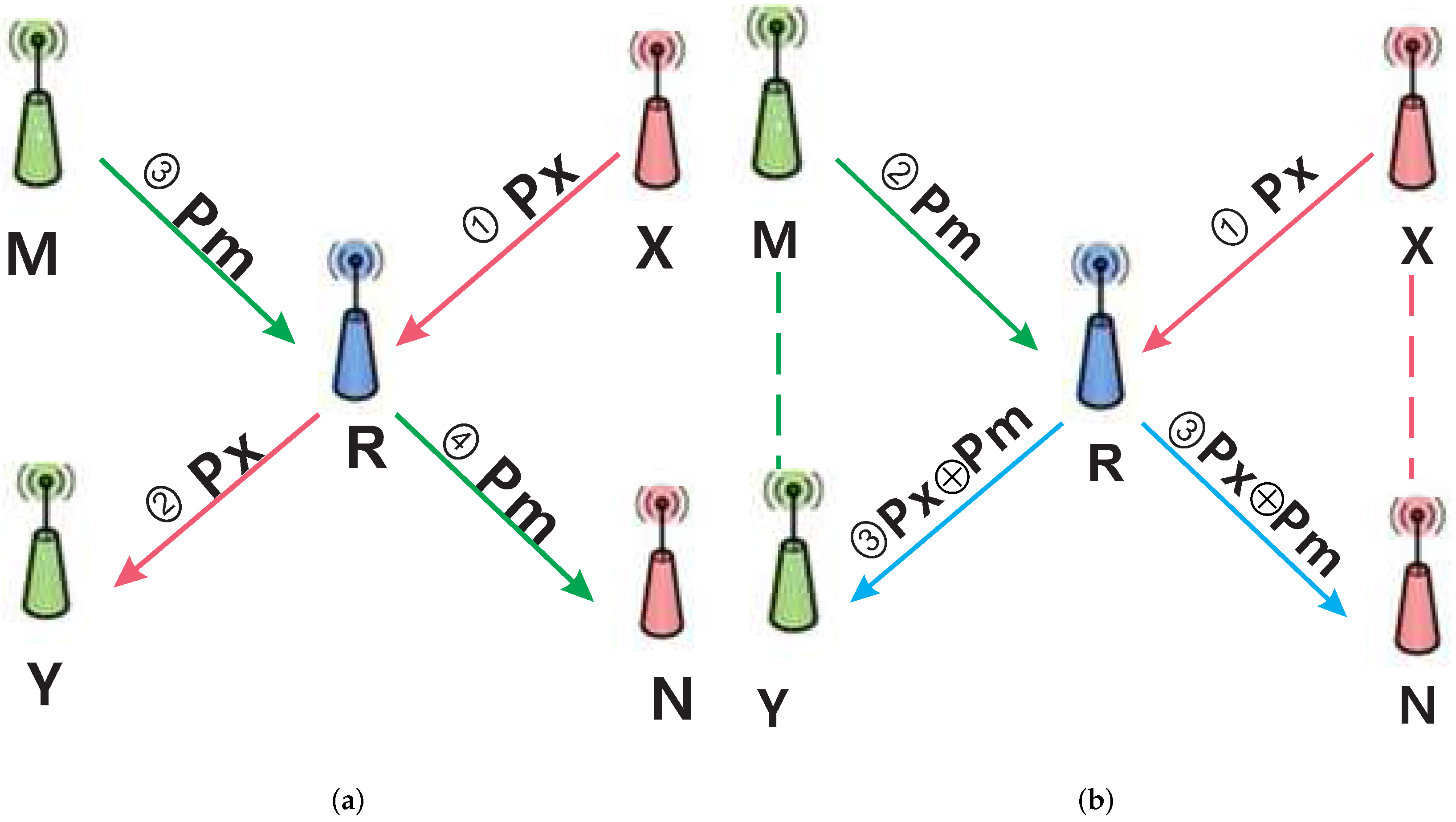
The principle of the network coding strategy can be illustrated by the following two typical models, “Alice-Bob structure” and “X structure” [8]. An “X structure” model is shown in Figure 1, in which the node X will forward the packet Px to the node Y through the router R, and the node M will forward the packet Pm to the node N through the router R. In general, the process is as following: X transmits Px to R, and then R stores Px and transmits it to Y; M transmits Pm to R, and then R stores Pm and transmits it to N. In the process, the total number of transmission is four. If a network coding scheme is applied to the transmission process, when X broadcasts Px to R, meanwhile N also receives Px; when M broadcasts Pm to R, meanwhile Y also receives Pm. After receiving Px and Pm, R will perform XOR on both them and broadcast the result to Y and N. Then Y performs XOR on the result and Pm received before, and gets Px that it should receive. Likewise, N can also get Pm which M sends to it. However, in this process, the total number of transmission is only three.

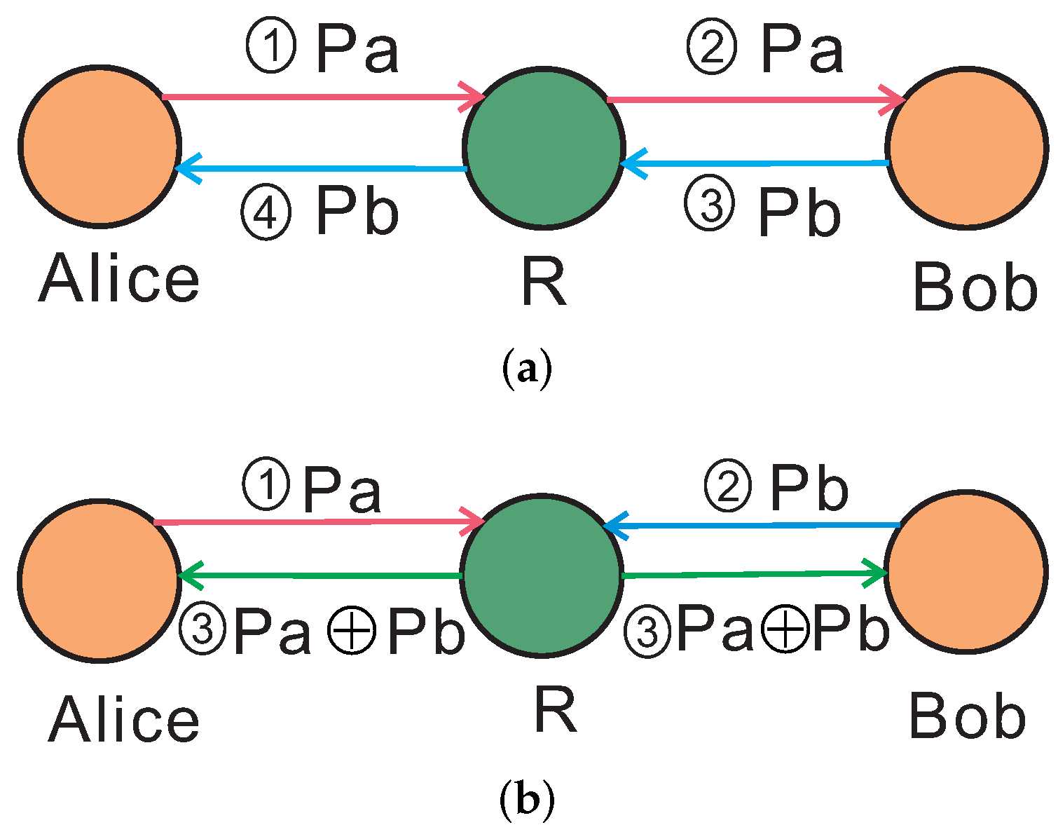
The other model, “Alice-Bob structure”, as shown in Figure 2. The node Alice will forward the packet Pa to the node Bob through the router R, and the node Bob will forward the packet Pb to the node Alice through the router R. Usually, the transmission process is as following: Alice transmits Pa to R, and then R stores Pa and transmits it to Bob; Bob transmits Pb to R, and then R stores Pb and transmits it to Alice. In the process, the total number of transmission is four. If a network coding scheme is used, the situation will be improved. Alice transmits Pa to R and Bob also transmits Pb to R. Then R performs XOR on Pa and Pb, and transmits the result respectively to Alice and Bob. Bob will get Pa by performing XOR on the result and its own Pb. Likewise, Alice will also get Pb. In the whole process, the total number of transmission is only three. Through decreasing the total number of transmission in a network which includes “Alice-Bob structure” or “X structure”, the low transmission delay and energy consumption and the high throughput can be obtained.

2). COPE made the following main contributions [13]:

(1)

It put forward a mechanism to monitor network coding opportunities. The mechanism uses the broadcast characteristics of wireless network to monitor the information of neighbor nodes and obtain the number of packets owned by the neighbor nodes. Then it determines whether to encode the received packets. It can maximize the amount of data in one transmission under ensuring that the neighbor nodes can completely decode and obtain the packets that they need.

(2)

It put forward an opportunistic coding mechanism. Whether a routing node encodes the received packets mainly depends the principle of coding. This principle must ensure that each next-hop node has enough data to decode the encoded packet after receiving it. The decoding conditions is as follows: Suppose that a node needs to transmit n packets $p_1,p_2,\dots ,p_n$ to the n next-hop nodes $r_1,r_2,\dots ,r_n$. The unique condition by which the node can encode the n packets is that every next-hop node $r_i$ has the other $n-1$ packets $p_j$($i\ne j$).

(3)

It proposed the concept of coding gain. COPE compared the number of transmission between the coding method and the non-coding method, and took the result as a reference standard for improving network performance, such as network throughput and so on. Based on this, it put forward the concept of coding gain. Coding gain is defined as the ratio of the number of transmission without network coding to the minimum number of transmission with the network coding in COPE. According to the definition, the ratio is greater than or equal to 1. For any network, the performance of unicast is still an unresolved problem in the traditional network coding [14]. In actual transmission, due to the availability of coding opportunities, the overhead of packet header and other reasons, the coding gain is often relatively lower.

3. The Problem

This paper proposes a perceptual routing decision model, named ANCR. Different from the previous models which require not only the same transmission success rate on all links, but also the same transmission success rate in two directions of each link, our model assumes that the transmission success rates on all links are different, and the transmission success rates in two directions of a link are also different. A network coding strategy is proposed under these new and more practical assumptions.

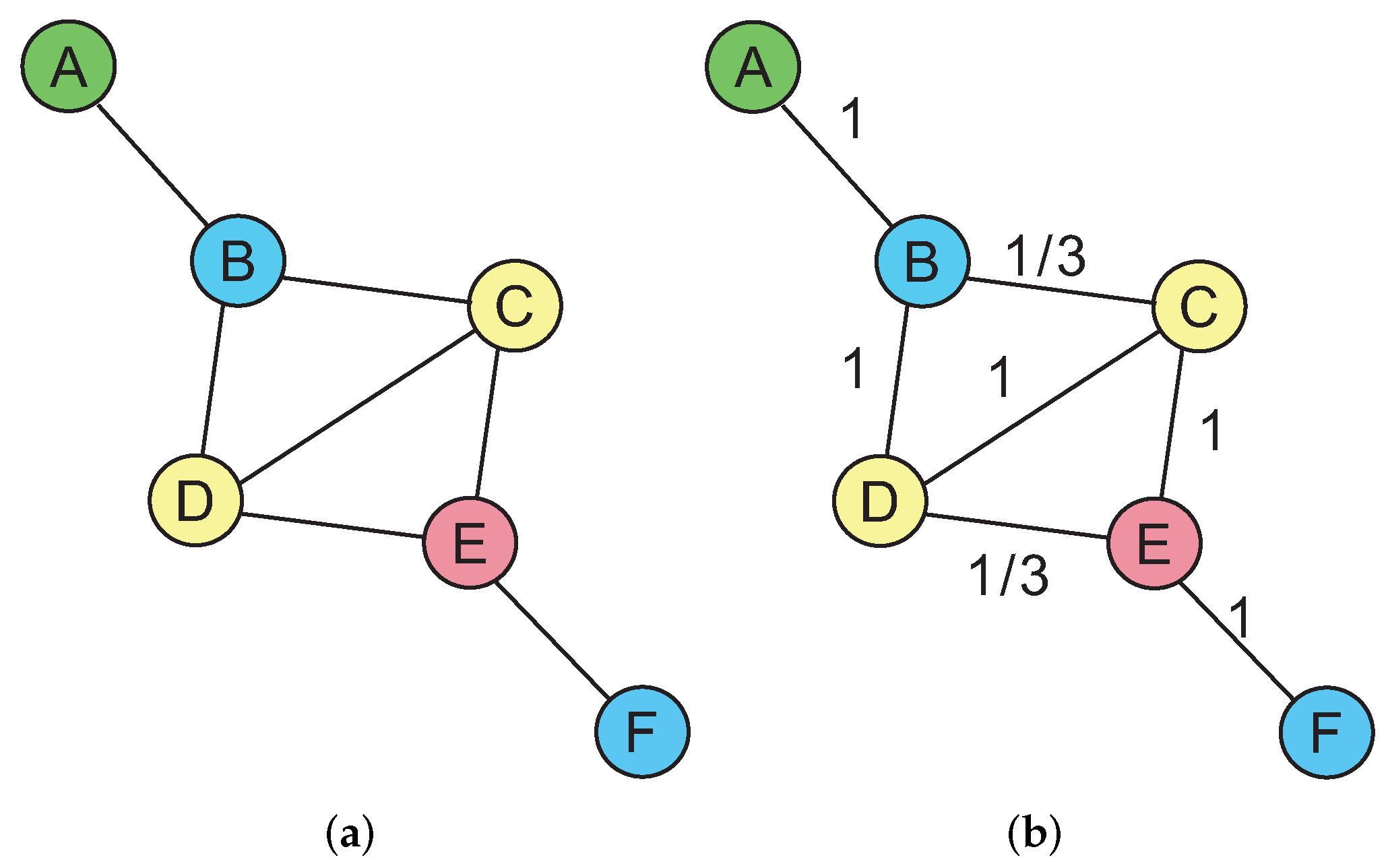
Here is an example, as shown in Figure 3a. It is assumed that the network meets the preconditions above-mentioned and the success transmission rates of all the links are all 100%. There are two data streams in two directions in the network. One is from the node A to the node E, whose path is $A\to B\to D\to E$, and the number of transmission is three. The other is from the node F to the node B, whose path is $F\to E\to C\to B$, and the number of transmission is three. Thus, finishing transmitting the two packets, the total number of transmission is six. Now, if we consider network coding opportunities and introduce the network coding strategy, the path from F to B will be changed to $F\to E\to D\to B$. It is obvious that D has a coding opportunity, which makes the number of transmission of the node D change from two to one. Thus, the total number of transmission changes to five and the network performance is promoted by about 17%.

However, in a real WSN, such as monitoring the environment where wildlife lives, military investigation and so on, link quality [15] is always affected by many unpredicted and uncertain external environmental factors, such as temperature, humidity and electromagnetic waves, etc [16]. In addition, the network’s own factors, such as the nodes’ transmitting power and working frequency, etc., also affect the link quality. These factors usually cause packet loss in data transmission processes [17,18]. Therefore, in an actual network, there are various transmission success rates on different links and in the two directions of a link, which makes the above-mentioned traditional network coding unusable. As shown in Figure 3a,b, they have the same network topology, but there is the different link quality in the latter (The numbers marked on each link represent the transmission success rate of the link. For example, the transmission success rate of the link BC is 1/3, which means that, on average, if the number of transmission is three, only once is successful.). Without considering the transmission success rates of the links and the coding opportunities, the optimal paths should be $A\to B\to D\to E$ and $F\to E\to C\to B$. However, retransmitting caused by unsuccessful transmission leads to the total number of transmission of the two data streams is ten $((1+1+3)+(1+1+3)=10)$. To introduce the coding opportunities, we need to appropriately adjust the paths. If the path $A\to B\to D\to E$ is not changed, the other path will be changed to $F\to E\to D\to B$. Then the node D has a new code opportunity. Unlike the network where there is no difference in link quality, the transmission success rate of the link DE is 1/3. So after calculating, the total number of transmission of the two data streams is nine $((1+1)+(1+3)+3=9)$ although D can encode the two packets from the different data streams into a big one and broadcast it to B and E. The network performance is improved by only 10%. Therefore, in a network with different-success-rate links, though the network coding strategy could be used, the improvement of the whole network performance would be discounted, due to the influence and restriction of the low link quality.

In order to solve the above problem, this paper proposes a routing decision model, named ANCR, which can sense network coding opportunities and use high-quality links to create coding opportunities to enhance the overall performance of a network. This approach not only passively applies the existing network coding opportunities as the traditional approaches [19], but also uses the high-quality links to create more coding opportunities. Its main idea is as following: When the quality of a link between two nodes is not good enough (as the link between D and E in Figure 3b), that is to say, in the case of different-success-rate links, we will use another node (as the node C in Figure 3b) which is linked with the two nodes and respectively has the better link quality as the forwarding node. In this way, the new forwarding node can have a coding opportunity to realize cooperative data forwarding. If there is a decrease in the number of transmission to bring an increase in the network throughput, then the whole network performance would be improved. Since the quality of the link CD is as good as that of the link CE, we take C as the intermediate forwarding node. So the initial path $A\to B\to D\to E$ will be changed to $A\to B\to D\to C\to E$, and the other initial path $F\to E\to C\to B$ will be changed to $F\to E\to C\to D\to B$. Then there are the coding opportunities at D and C. The total number of transmission is only six (the statistical result for multiple transmission tasks [12]). Compared with the previous strategy that uses D as the forwarding node, the total number of transmission is reduced by three. The direct effect is that the transmission time and the energy consumption of the nodes are all saved. The indirect effect is that the network throughput is improved.

4. Overview

In this paper, according to the real relevant parameters in the WSN employed for monitoring wild animals in Qinling region in China, which was deployed by our lab, we establish the network topological graph and the data stream model. The specific parameters are as follows: 150 nodes deployed randomly in an area of about 1 square kilometers; the transmission distance of a single link is 80 m; the link bandwidth is 250 Kbps; the transmission success rate of a link is between 0 and 1; the number of data streams is from 0 to 30. Then, the simulations of NCR and ANCR are carried out. The simulation results show that, compared with the NCR strategy, ANCR can reduce the network delay by about 50% and increase the network throughput by about 66.67%. With the increase of network data streams, the advantage of saving energy of ANCR becomes more and more obvious.

In order to verify the performance of ANCR, the following steps of the simulation are carried out in the paper:

(1)

ANCR establish a network topological graph firstly. Then, the graph is symbolized and represented by an appropriate data structure. This step will be described in detail in Section 5.1.

(2)

ANCR establish a data stream model secondly. Then, the data stream model is symbolized and represented by an appropriate data structure. This step will be described in detail in Section 5.2.

(3)

The number of network nodes, the number of data streams and the number of packets are initialized respectively.

(4)

NCR is used to make routing decisions and the related parameters are calculated. The link selection criteria is defined as the smaller expected transmission count(ETX) [20]. The neighborhood search is performed on the route selected by NCR. The specific neighborhood search algorithm will be described in Section 7.

(5)

Calculate the related parameters about the current route and go to the next step.

(6)

If you want to experiment on other scenes, initialize again the number of network nodes, the number of data streams and the number of packets and back to the step (4). Otherwise, finish the experiment.

The following sections will describe the settings of a simulation scene, the algorithm design and so on.

5. Network and Data Stream

In order to carry out the simulation, we establish the network topological graph and the network data stream model in the paper firstly. Then we need to represent the network and data stream into the computer to simulate nodes, links, and states in real network.

5.1. Representation of Network Topology

The network topology can be defined by the nodes and the corresponding links between the nodes in a given network. Whether a link between two nodes exists depends on whether each node of them is within the direct transmission range of the other. In this way, a network topological graph $G=(N,E)$ can be built, where N denotes the set of the network nodes and E denotes the set of the links directly connecting two nodes in the network. Each node in the network may be the source or destination node of a data stream. The set of the input links of the node i is denoted by $E^{-}(i)$ and the set of the output links of the node i is denoted by $E^{+}(i)$. The link that directly connects the node i to the node j is denoted by $e=(i,j)$. $\overline{e}=(j,i)$ denotes the reverse path of the link e ($e=(i,j)$).

For a path P and a link e, we use $e\in P$ to denote that the link e is in the path P. $e_1{e}_2\in P$ represents that the link $e_1$ and the link $e_2$ are all in the path P and $e_2$ is the subsequence of $e_1$. For a path P and a node i, $i\in P$ denotes the node i is in the path P.

$d_{ij}$ is the distance between the nodes i and j. $l_i$ represents the communication radius of the node i. On a single channel, whether the transmission from the node i to the node j is successful is discussed in two cases: (1) If $d_{ij}\le l_i$, then the transmission will be successful; (2) If $d_{ij}>l_i$, then the transmission will be unsuccessful.

Each link $e\in E$ corresponds to a transmission success rate $t(e)$ representing the success probability of data transmission on the link e. If a link is $e=(i,j)$, then the transmission success rate of the link is defined as $t(e)=t(i,j)$. If there is an intermediate node r, the source node i can send a packet to the destination node j through the node r, then this path can be expressed as $P=(i,r,j)$, which represents that the direction of the data stream is $i\to r\to j$, the transmission success rate of the path is $t(P)=t(i,r,j)=t(i,r)*t(r,j)$.

If $t(i,r,j)>t(i,j)$, it is indicated that the transmission quality of the path $i\to r\to j$ is good and better than that of the direct link between the node i and the node j. Then the network topological graph $G=(N,E)$ will be modified as following: The direct link between the node i and the node j is deleted. The path $P=(i,r,j)$ is remained in the graph G. The changes of the link quality will lead to updating the network topological graph. In addition, to add or remove some nodes in the network will also lead to updating the network topological graph. In an actual deployment, whether outdoors or indoors, the nodes and the quality of the links in the network may need to be updated due to the battery exhaustion of nodes, nodes sleep, outside interference, the redeployment of nodes or the new nodes waked up or added, etc. So we need an update mechanism of network topological graph.

The graph $G=(N,E)$ indicates a network state at a certain moment. $G_0=(N_0,E_0)$ denotes the initial network state. $G_t=(N_t,E_t)$ denotes the network state at time t. $\Delta N_t$ and $\Delta E_t$ respectively represent the set of nodes and the set of links added or deleted from the original network from time 0 to time t due to the changes of the network state. So $\Delta G_t$ = ($\Delta N_t$ , $\Delta E_t$) indicates the changes of the network state during the period of $\Delta t$. The cases of adding and removing nodes are discussed as follows:

Adding nodes: This case refers to that a node restarts to work in the network or a new node is added to the network. After a node is added, the links between the added nodes and its neighbor nodes should be first established, and then the network topological graph should be updated. At the same time, the states of the related nodes and the transmission success rates of the related links should be updated correspondingly.

Removing nodes: This case refers to that a node starts to sleep in the network or a node is removed from the network. After a node is removed, the links between the removed node and its neighbor nodes should be first deleted, and then the network topological graph should be updated. At the same time, the states of the related nodes and the transmission success rates of the related links should be updated correspondingly.

5.2. Representation of Path and Data Stream

The definition of the data stream model of network is used to obtain a feasible path under a known network topological graph. Firstly, a network topology is represented by a correlation matrix $A\in R^{V\times L}$ of nodes and links, where V denotes the total number of nodes and L denotes the total number of links. In the matrix, the element $a_{ij}$ represents the relationship between the node i and the link j:

$$a_{ij}=\left\{\begin{array}{cc}\hfill 1,& if{e}_j\in E^{+}(i)\hfill \\ \hfill -1,& if{e}_j\in E^{-}(i)\hfill \\ \hfill 0,& others\hfill \end{array}\right.$$

(1)

where $E^{-}(i)$ and $E^{+}(i)$ respectively represent the input and output links of the node i.

If a path successively includes the following links $e_1,e_2,\dots ,e_n$, then the path would be defined as $P=e_1{e}_2\dots e_n$. $X(P)$ is a vector whose length is L ($X(P)\in R^L$). For the ith element in $X(P)$:

$$x_i(P)=\left\{\begin{array}{cc}\hfill 1,& if{e}_i\in P\hfill \\ \hfill 0,& others\hfill \end{array},1\le i\le L\right.$$

(2)

For a data stream k, it can be expressed as a vector $U_k\in R^V$. For the ith element in $U_k$:

$$u_i=\left\{\begin{array}{cc}\hfill 1,& i=s(k)\hfill \\ \hfill -1,& i=d(k)\hfill \\ \hfill 0,& others\hfill \end{array},1\le i\le V\right.$$

(3)

where $s(k)$ and $d(k)$ respectively represent the source and destination nodes of the data stream k. Because the path $P_k$ of the data stream k must satisfy the limitation: $AX(P_k)=U_k$, a set of potential paths of the data stream k can be obtained. All the possible solutions of $X(P_k)$ are just the potential paths.

6. Optimization of Routing Decision in WSNs with Different-Success-Rate Links

6.1. Metric of Link Quality

Since ETX can easily characterize network throughput and energy consumption of nodes, and also affect end-to-end delay, this paper selects it as the path selection criteria in the case of considering coding opportunities to find a high-throughput path in a network with different link quality.

The minimum ETX of forwarding a packet from a source node to a destination node (including the number of retransmission) is used as the path selection criteria. The ETX of a link is calculated based on the transmission success rate of the link, for example, the ETX of a link whose transmission success rate is 50% is two. The ETX of a path is the sum of the ETXs of all the links included in the path, for instance, the ETX of a path containing three lossless links is three.

The transmission success rate of a link is calculated by the forward and reverse transmission success rates of the link. The forward transmission success rate $q_f$ is the successful probability of delivering a packet to the receiver. The reverse transmission success rate $q_r$ is the successful probability of receiving an acknowledgment packet ACK from the sender. Therefore, the transmission success rate of the link is $q_r\times q_f$. If the sender does not receive the acknowledgment ACK from the receiver, the packet will be retransmitted. Since each attempt to transmit a packet can be viewed as a Bernoulli experiment, the ETX of the link is $1/(q_r\times q_f)$.

In addition, for the measurement of transmission success rate, the forward and reverse transmission success rates $q_f$ and $q_r$ are measured by using a dedicated link probe packet. Each node broadcasts a dedicated link probe packet with a fixed size every $\tau$ seconds. In order to avoid synchronization, there is a jitter ($\pm 0.1\tau$ seconds) in each probing. Each node needs to store the probe packets received in the last $win$ seconds. Nodes can be allowed to calculate their successful transmission probabilities at any time $t_i$:

$$q(t_i)=count(t_i-win,t_i)/(win/\tau )$$

(4)

where $count(t_i-win,t_i)$ represents the number of probe packets received during the last $win$ seconds, and $(win/\tau )$ indicates the number of probe packets that should be received when the transmission links are lossless. In general, when the link direction is $A\to B$, the node A can measure the transmission success rate $q_r$, and the node B can measure the transmission success rate $q_f$. Since the node B defaults to receiving a probe packet from the node A every $\tau$ time intervals, it can accurately calculate the current transmission success rate $q_f$ according to the number of the packets actually received and that should be received. In this way, the node A can also get the current transmission success rate $q_r$. To calculate the ETX of a link needs $q_f$ and $q_r$ simultaneously. Each probe packet sent by the node A contains the number of probe packets received by the node A from its each neighbor node in the last $win$ seconds. So this can allow the node B to be also able to calculate $q_r$ whenever a probe packet from the node A is received by the node B. Likewise, the node A can also get $q_f$. In a word, all nodes can obtain the corresponding $q_f$ and $q_r$ of the related links and calculate the transmission success rates and ETXs of the links.

6.2. Establishment of ANCR Model

The problem of minimizing transmission count by using network coding is formulated. Suppose that in a wireless network, there has already existed K data streams, now, H new data streams are added into the network. For a new data stream h ($1\le h\le H$), its source and destination nodes are respectively $s(h)$ and $d(h)$. If a path $P\in R_h$ is selected, where $R_h$ is the potential path set of the data stream h, then $f_h(P)=1$, otherwise $f_h(P)=0$. $P_h$ denotes the path of the data stream h. $M_h$ denotes the set of nodes on the path $P_h$. M denotes the set of nodes on the paths of all the H data streams. $1/t(e_j)$ denotes the ETX of the link $e_j$, where $t(e_j)$ denotes the transmission success rate of the link $e_j$. We use $T_i^{\{e\}},\forall e\in E^{+}(i),i\in N$ (N represents the node set of the network) to denote the sum of the transmission counts caused by transmitting packets through all the output links of the node i. For a link $e=(i,j)$, $\overline{e}=(j,i)$ denotes its reverse link.

The following optimization solution aims to minimize the ETX of the paths for all the incoming data streams under the given conditions, such as the data stream conservation, network coding and competition constraint, etc. Specifically, the model is as follows.

Minimum

$${\displaystyle \sum _{i\in M}{T}_i^{\{e\}},\forall e\in E^{+}(i),M=\bigcup _{h=1}^H{M}_h,M_h=\{m|\forall m\in P_h\}}$$

(5)

Subject to

$$\sum _{P\in R_h}{f}_h(P)=1,\forall 1\le h\le H,f_h(P)=\left\{\begin{array}{cc}\hfill 1,& ifPisselectedasthepathofthedatastreamh\hfill \\ \hfill 0,& others\hfill \end{array}\right.$$

(6)

$$T_i^{\{e_1,e_2\}}\le \sum _{k=1}^K\sum _{\overline{e_1}{e}_2\in P}\sum _{j=1}^3\frac{1}{t(e_j)}+\prod _{j=1}^{3}sgn[t(e_j)]\times \sum _{h=1}^H\sum _{\overline{e_2}{e}_1\in P}{f}_h(P)[\sum _{j=1}^3\frac{1}{t(e_j)}],\forall e_1,e_2\in E^{+}(i),i\in N$$

(7)

$$T_i^{\{e_1,e_2\}}\le \sum _{k=1}^K\sum _{\overline{e_2}{e}_1\in P}\sum _{j=1}^3\frac{1}{t(e_j)}+\prod _{j=1}^{3}sgn[t(e_j)]\times \sum _{h=1}^H\sum _{\overline{e_1}{e}_2\in P}{f}_h(P)[\sum _{j=1}^3\frac{1}{t(e_j)}],\forall e_1,e_2\in E^{+}(i),i\in N$$

(8)

$$\begin{array}{c}\hfill T_i^{\{e\}}\le {\displaystyle \prod _{j=1}^3}sgn[t(e_j)]\times {\displaystyle \sum _{h=1}^H}{\displaystyle \sum _{e\in P,s(h)=i}}{f}_h(P)[{\displaystyle \sum _{j=1}^3}\frac{1}{t(e_j)}]+{\displaystyle \sum _{k=1}^K}[{\displaystyle \sum _{e\in P_k,s(h)=i}}{\displaystyle \sum _{j=1}^3}\frac{1}{t(e_j)}+\\ \hfill {\displaystyle \sum _{e_1\in E^{-}(i)}}{\displaystyle \sum _{k=1}^K}{\displaystyle \sum _{e_{1}e\in P}}{\displaystyle \sum _{j=1}^3}\frac{1}{t(e_j)}+{\displaystyle \sum _{h=1}^H}{\displaystyle \sum _{e_{1}e\in P}}{f}_h(P)[{\displaystyle \sum _{j=1}^3}\frac{1}{t(e_j)}]-T_i^{\{e,\overline{e_1}\}}],\forall e\in E^{+}(i),i\in N\end{array}$$

(9)

$$AX(P_h)=U_h,\forall 1\le h\le H$$

(10)

• Constraint (6) denotes the path selection constraint, which means that from the source node to the destination node, a data stream h has one and only one path to select in the set $R_h$ of potential paths determined by the constraint (10).
• Constraints (7) and (8) denote the constraints for the maximum ETX of broadcast transmission of the node i carrying out network coding. Constraint (7) denotes the constraint for the maximum ETX of the path $\overline{e_2}{e}_1$. Constraint (8) denotes the constraint for the maximum ETX of the path $\overline{e_1}{e}_2$. When the variable of the sign function $sgn$ is 0 (the transmission success rate of a link is 0), which indicates that the link can not be used, the value of the sign function is 0. At this moment, the last parts of the right of the two inequalities are all 0, which means that there is only one-way transmission limitation. In this case, if $T_i^{\{e_1,e_2\}}$ needs to simultaneously satisfy the constraints (7) and (8), $T_i^{\{e_1,e_2\}}$ must be 0. Since the bidirectional unreachable link is not within the optimization range of the optimization equation, the sign function constrains the coding opportunity of unidirectional unreachable links.
• Constraints (9) shows the ETX of unicast transmission of raw packets transmitted by the node i.
• Constraints (10) limits the potential paths of the data stream h. All the possible solutions of $X(P_h)$ are just the potential paths.

7. Approximation Algorithm

It is a NP-hard problem [21] to compute the minimum transmission count in the case of various link quality. Given a graph $G(V,E)$, an independent set of G is a set of vertices where there is no edge between any two vertices. The maximum independent set problem is a known NP-hard problem. To solve the minimum transmission count can be converted to a maximum independent set problem. So to solve the minimum transmission count is also NP-hard.

The main proof process is as follows: In a graph $G(V,E)$, we specify two nodes as the source and destination nodes. Each edge is a corresponding link between two related nodes. The link capacity between any two nodes is assumed to be one unit. It is assumed that there are conflicts between the links. Therefore, the minimum transmission count can be obtained only after the sequence of the maximum independent set of the graph G is arranged. That is to say, to solve the minimum transmission count of a network is equivalent to solve the maximum independent set of the graph established on the network. The latter is a known NP-hard problem. So the former is also a NP-hard problem.

Therefore, we use a local search heuristic to adjust routing paths in partial section to minimize the transmission count. As discussed in Section 3, in order to get a network coding opportunity, we need to modify the local path(s) near a cross node where two data streams’ paths intersect. In addition, the "Alice-Bob structure" or "X structure" coding opportunity can be found at least in a two-hop communication range. Thus we choose a cross node as a center and take its one-hop communication range as the neighborhood range to carry out the local search heuristic.

The neighbor search algorithm includes two primary steps as follows: (1) to determine the initial path of each data stream: The algorithm takes the transmission success rate of each link as the weight, and generates a new path for each data stream by finding the path on which the sum of weights of the links is maximum (the ETX is minimum); (2) to optimize the initial paths: The algorithm adjusts (or creates) a cross node for the initial paths so that the sum of the ETXs of all the paths passing through the cross node decreases and the total number of transmission in the network is as small as possible. The specific implementation process is shown in

Table 1. Main part of optimal local path Algorithm.

No.	Sentence of Algorithm
1:	$\mathbf{if}$ node v is a cross node;
2:	L(v) = $\varphi$;
3:	compute $E(Int)$ of two local paths: $p_1\to v\to n_1$, $p_2\to v\to n_2$;
4:	$\mathbf{for}$ each v’s neighbour node a;
5:	$\mathbf{if}$ ${\alpha }_{a,v}<{\alpha }_{p_2,v}$ $\mathbf{then}$
6:	there is a local path strategy $St$: $p_1\to a\to n_1$, $p_2\to a\to v\to n_2$;
7:	$E(St)$ = $max({\alpha }_{p_1,a},{\alpha }_{p_1,v})+max({\alpha }_{p_2,a},{\alpha }_{p_2,n_1})$ $+max({\alpha }_{a,n_1},{\alpha }_{a,v})+{\alpha }_{v,n_2}$;
8:	$\mathbf{if}$ $E(Int)>E(St)$ $\mathbf{then}$
9:	$L(v)=L(v)+St$;
10:	$\mathbf{end}$ $\mathbf{if}$
11:	$\mathbf{end}$ $\mathbf{if}$
12:	$\mathbf{if}$ ${\alpha }_{v,a}<{\alpha }_{v,n_2}$ $\mathbf{then}$
13:	there is a local path strategy $St$: $p_1\to a\to n_1$, $p_2\to v\to a\to n_2$;
14:	$E(St)$ = $max({\alpha }_{p_1,a},{\alpha }_{p_1,n_2})+max({\alpha }_{v,a},{\alpha }_{v,n_1})$ $+max({\alpha }_{a,n_2},{\alpha }_{a,n_1})+{\alpha }_{p_2,v}$;
15:	$\mathbf{if}$ $E(Int)>E(St)$ $\mathbf{then}$
16:	$L(v)=L(v)+St$;
17:	$\mathbf{end}$ $\mathbf{if}$
18:	$\mathbf{end}$ $\mathbf{if}$
19:	$\mathbf{end}$ $\mathbf{for}$
20:	get $l(v)$ and use $l(v)$ as new local paths;
21:	$\mathbf{else}$ $\mathbf{if}$ node v is a pseudo cross node $\mathbf{then}$
22:	$L(v)=\varphi$;
23:	compute $E(Int)$ of two local paths: $p_1\to n_1$, $p_2\to$ $v\to n_2$;
24:	there is a local path strategy $St$: $p_1\to v\to n_1$, $p_2\to$ $v\to n_2$;
25:	$E(St)$ = $max({\alpha }_{p_2,v},{\alpha }_{p_2,n_1})+max({\alpha }_{p_1,v},{\alpha }_{p_1,n_2})$ $+max({\alpha }_{v,n_2},{\alpha }_{v,n_1})$;
26:	$\mathbf{if}$ $E(Int)>E(St)$ $\mathbf{then}$
27:	$L(v)=L(v)+St$;
28:	$\mathbf{end}$ $\mathbf{if}$
29:	$\mathbf{for}$ each v’s neighbour node a $\mathbf{do}$
30:	there is a local path strategy $St$: $p_1\to a\to n_1$, $p_2\to a\to n_2$;
31:	$E(St)$ = $max({\alpha }_{p_2,a},{\alpha }_{p_2,n_1})+max({\alpha }_{p_1,a},{\alpha }_{p_1,n_2})$ $+max({\alpha }_{a,n_2},{\alpha }_{a,n_1})$;
32:	$\mathbf{if}$ $E(Int)>E(St)$ $\mathbf{then}$
33:	$L(v)=L(v)+St$;
34:	$\mathbf{end}$ $\mathbf{if}$
35:	$\mathbf{end}$ $\mathbf{for}$
36:	get $l(v)$ and use $l(v)$ as new local paths;
37:	$\mathbf{end}$ $\mathbf{if}$

, where a cross node refers to the node through which there are at least two paths of data streams; a pseudo cross node is such a node that belongs to only one path and whose neighbor nodes belong to another path, or that can be added to another path as a transit node.

To illustrate the algorithm clearly, some symbols are defined as follow:

• v: a current node.
• $Int$: an initial local path strategy.
• $St$: a local path strategy of node v with network coding.
• $E(St)$: the sum of the ETXs of a local path strategy $St$.
• $L(v)$: a collection of local path strategies of node v.
• a: a neighbor node of the current node v.
• $l(v)$: a local path strategy $St$ that makes $E(St)$ minimum in $L(v)$.
• $p_i$: the predecessor node of the current node v in the path of a data stream i.
• $n_i$: the successor node of the current node v in the path of a data stream i.
• ${\alpha }_{i,j}$: the ETX of a link between the nodes i and j.

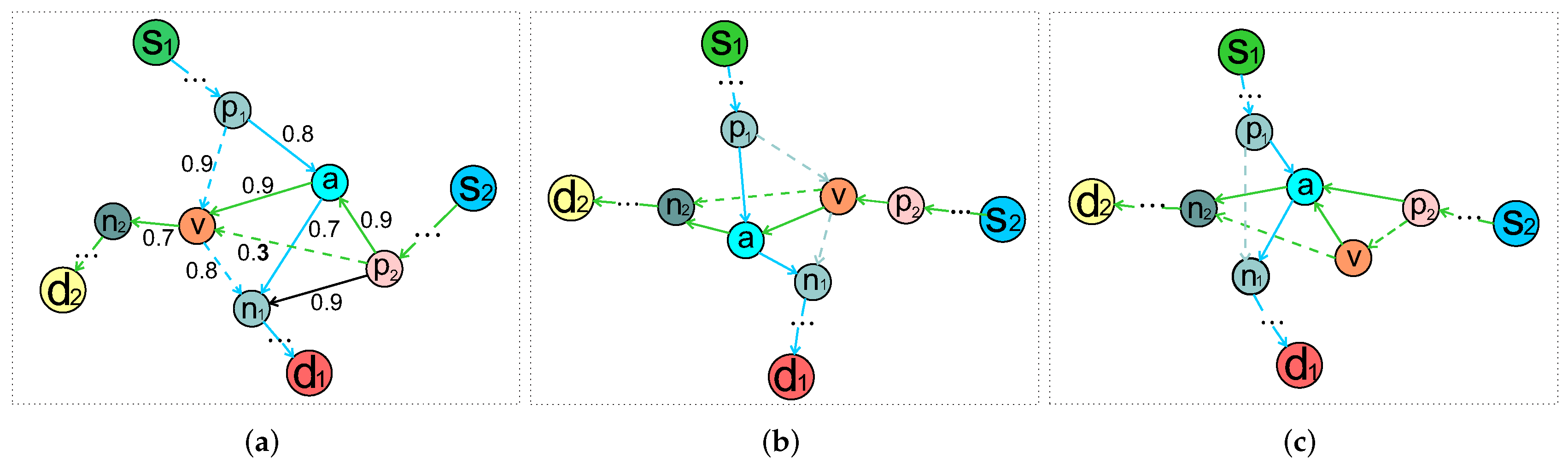
Three main cases dealt with by the algorithm are shown in Figure 4. Suppose that the current node is v. Figure 4a indicates the case that the quality of the current node v’s input link (e.g., $p_2$,v) is poor. In the figure, there are two paths $s_1,\dots ,p_1,v,n_1,\dots ,d_1$ and $s_2,\dots ,p_2,v,n_2,\dots ,d_2$, which respectively belong to two data streams passing through the cross node v, and the transmission success rates of the related links are marked. By calculating, for the first data stream, the node v is replaced with its neighbor node a; for the second data stream, the direct transmitting from the node $p_2$ to the node v is instead of the forwarding through the node v’s neighbor node a. Then the sum of the ETXs of the new paths $s_1,\dots ,p_1,a,n_1,\dots ,d_1$ and $s_2,\dots ,p_2,a,v,n_2,\dots ,d_2$ is much smaller. Therefore, this local path strategy should be used as an alternative local path strategy to adjust the routing paths associated with the current node. Figure 4b illustrates the case that the quality of the current node v’s output link (e.g., v,$n_2$) is poor, and gives an alternative local path strategy. Figure 4c shows the case that the current node v has no any coding opportunity, and gives an alternative local path strategy with a coding opportunity.

8. Simulation and Evaluation

In this section, we evaluate the performance of our routing approaches using Java. According to the specific parameters: 150 nodes are randomly deployed in the area of about 1 square kilometers in area; a single link transmission distance is 80 m; the link bandwidth is 250 Kbps; a link transmission success rate is between 0 and 1; the data stream from 0 to 30. We build a simulation environment and simulate it.

8.1. Delay Analysis

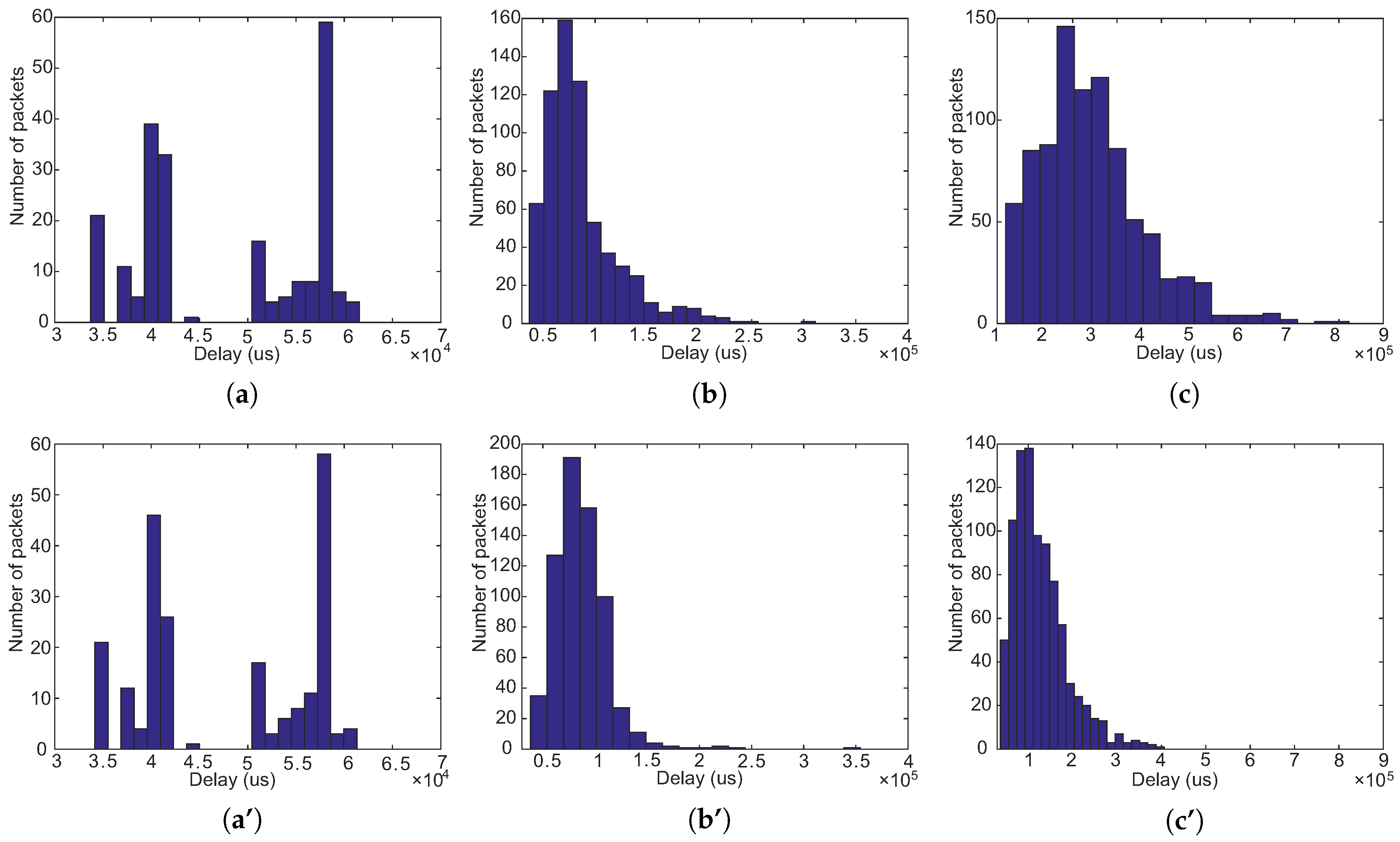
In the simulation, all the source and destination nodes of each data stream are chosen randomly and all the packets are generated randomly. Figure 5a,a’ show the comparison of delay distributions of 220 packets between NCR and ANCR in the case of two data streams. Because there are only two data streams, the network coding opportunities are fewer. ANCR degenerates to NCR, which makes NCR and ANCR have a similar delay distribution of 220 packets. Figure 5b,b’ show the comparison of delay distributions of 660 packets between NCR and ANCR in the case of five data streams. From the figures, we could find the packets with a longer delay in ANCR are slightly fewer than those in NCR. In spite of this, the fewer data streams still result in the fewer coding opportunities, so NCR and ANCR also have a similar delay distribution of 660 packets. Figure 5c,c’ show the comparison of delay distributions of 880 packets between NCR and ANCR in the case of twenty data streams. Intuitively, with the number of data streams increasing, both the number of intersections of data streams and the network coding opportunities are also raising. In addition, compared with NCR, ANCR would select a route with a high transmission success rate and coding opportunities, which can reduce the number of retransmission. Moreover, the coding technology can decrease the queuing delay of packets. All these reasons make ANCR bring about lower delay. The two figures also prove this conclusion. The center position of the distribution in NCR is about 2 $\mathsf{\mu }$s, however, that in ANCR is about $1\mathsf{\mu }$s. Therefore, compared with NCR, ANCR can reduce the network delay by about 50%.

8.2. Throughput Analysis

ANCR proposed in this paper is to maximize the network throughput by minimizing the total number of transmission of the network. In this part, we compare the performance of NFC and ANCR in increasing network throughput and analyse ANCR in improving the performance.

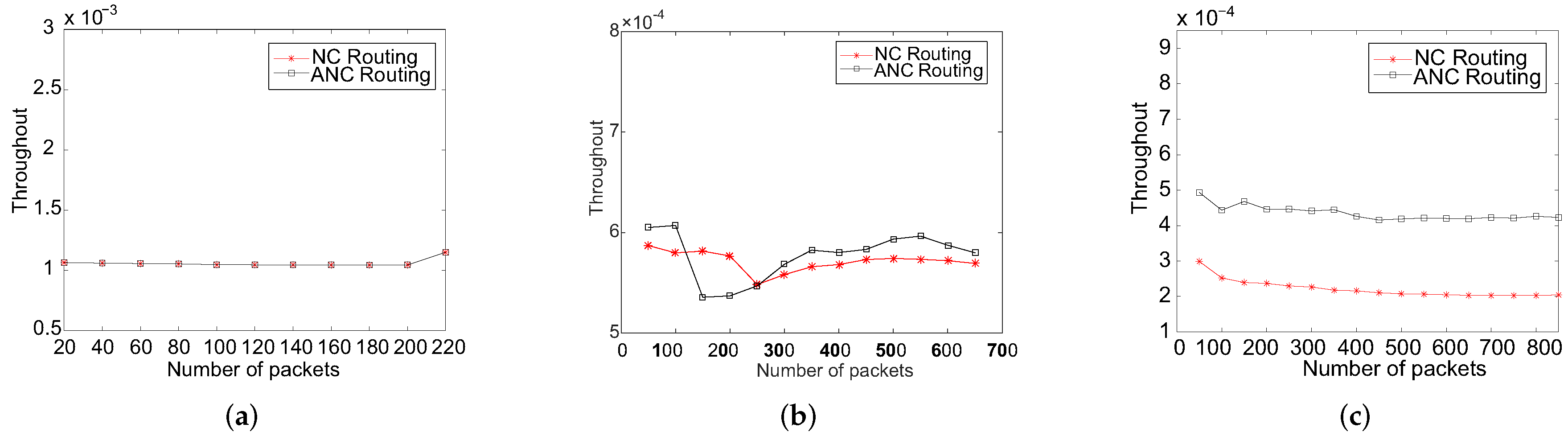
Figure 6 shows the comparison of network throughput between NCR and ANCR under the number of data streams and packets increasing respectively. In Figure 6a, there are only two data streams having no intersections, which is the worst case that ANCR is faced with, so the two approaches have the same performance. When the number of data streams is five, we can find the difference from Figure 6b. It shows when the number of packets is in the range of 100 to 250, the throughput of ANCR is lower than that of NCR. The main reason is that in the initial stage, ANCR needs to arrange the transmission time, which means that some packets need to wait for the other packets to participate in coding together (the waiting time is set to 3 $\mathsf{\mu }$s). There is a time delay compared with NCR. However, with the number of packets increasing, the time to wait for coding is gradually reducing and tending to be stable. When the number of packets of each data stream increases to greater than 250, the throughput of ANCR performs better than that of NCR. In Figure 6c, it is clearly indicated that ANCR has the better throughput than NCR in the case of the twenty data streams. The throughput of ANCR is about 2 times that of NCR. The main reason is analysed as following: Compared with NCR, when ANCR is used in a network having a large number of data streams, more network coding opportunities would be generated. In addition, with the increasing of packets at the node having a coding opportunity, the number of transmission of ANCR decreases more significantly than that of NCR. This directly leads to a greater improvement of the network throughput.

8.3. Energy Analysis

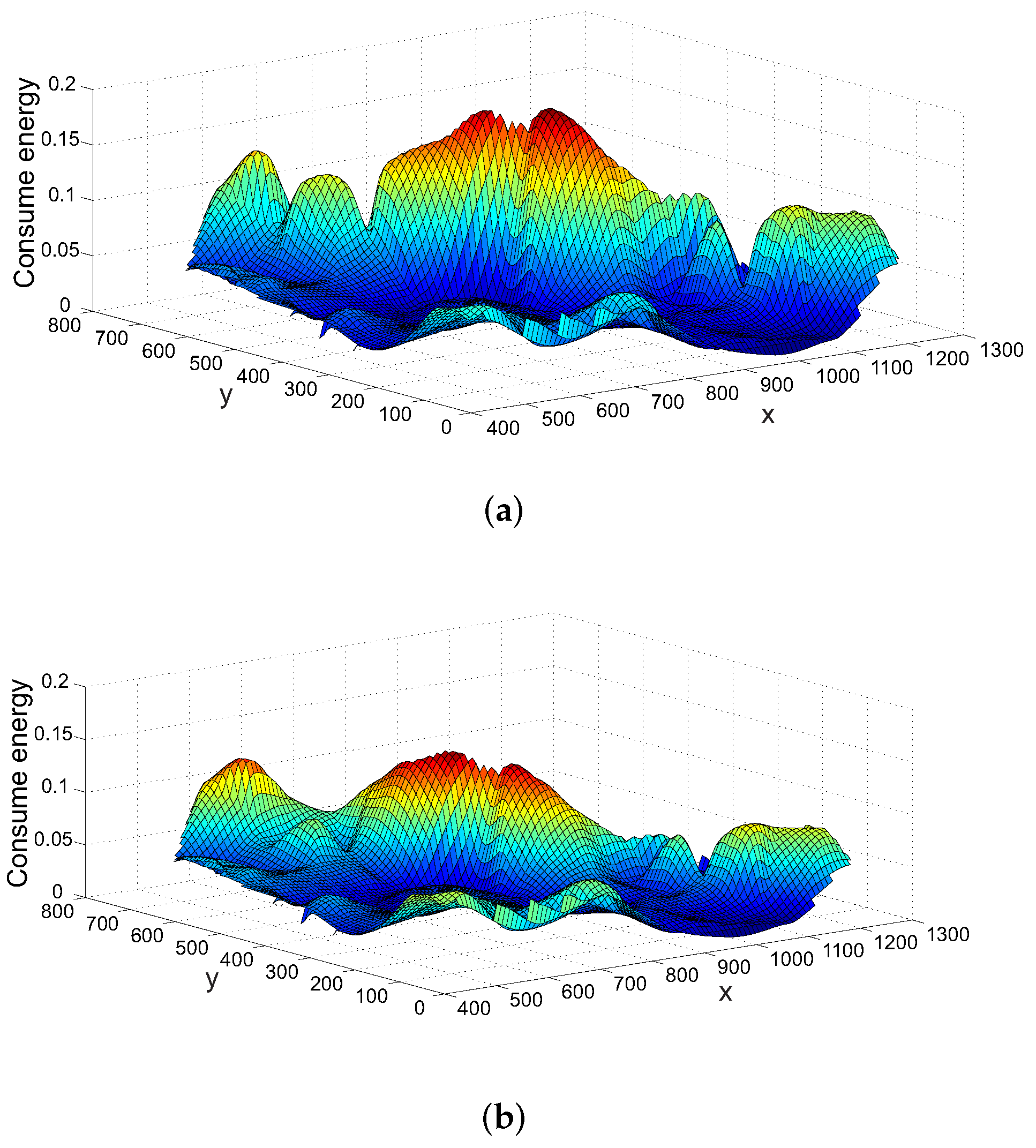
In this part, we focus on and analyse the energy consumption of nodes by using NCR and ANCR respectively to finish the transmission of 1000 packets in the case of thirty data streams. Figure 7 shows the energy consumption of nodes under using NCR and ANCR respectively. The X-axis and Y-axis represent the geographical location of nodes and the vertical axis represents the energy consumption of nodes. We define the initial energy of each node as $0.2$.

From Figure 7, we can come to the conclusion that the energy consumption of ANCR is less than that of NCR. The main reason is that ANCR chooses the nodes with coding opportunities and high transmission success rates to encode packets and transmit them, but NCR only considers the coding opportunities of nodes and ignores the transmission success rates of the nodes. Consequently, under the same network situation, the total number of transmission of ANCR is less than that of NCR, which means that the energy consumption of ANCR is lower than that of NCR. Moreover, the nodes whose energy consumption decreases all have coding opportunities.

In a word, with the number of data streams and packets increasing, the advantage of ANCR is becoming more and more obvious.

9. Related Works

In the early routing mechanisms which take network coding as the core, the implementation of network coding and the route selection were separated from each other. The path-given network coding algorithms were always adopted. In this kind of algorithm, coding opportunities are found by identifying the nodes that different data streams pass through in given routes and coding is implemented at these nodes. With the deep study of network coding, more coding opportunities can be created by dynamically adjusting routes.

Subsequently, many coding algorithms based on dynamically adjusting routes appear. They are mainly based on COPE scheme [12]. COPE constructs a network coding architecture under a given routing mechanism, whose main idea is to raise the amount of information of a forwarded packet. A router selects those packets that can be encoded together and “merges” the packets from different source nodes into a big one and sends it out.

In the COPE scheme, seeking network coding opportunities is mainly focused on. It requires that a node can perform a coding operation just when the node has an “X” or “Alice-Bob” structure coding opportunity, otherwise, COPE is as the same as a traditional routing mechanism.

Based on COPE, many researchers gave more detailed discussions on the coding method of path dynamic adjustment under different environments and backgrounds [8,22,23,24,25].

Widmer, J. et al. [23] proposed a routing selection method based on COPE, which designed a routing mechanism to promote network coding opportunities by discussing the constraints of different transmission rates and bandwidths in a network.

Zhang, J. et al. [8] built a throughput theory model by considering various transmission rates in a wireless network. By calculating the maximum throughput of unicast transmission, this approach controls routing selection and balances network coding opportunities with the use of high-rate links.

NCR [14], a routing strategy for wireless network environments, was put forward by Sengupta in MIT. For random and nonrandom monitoring modes, from a theoretical point of view, [14] analysed how to optimize the traffic in a wireless network using COPE. Different transmission rates are taken into account in particular in this strategy. However, this approach, as the same as the mentions in [8,23], also requires that in a wireless network, all the links have the same transmission success rate and there is the same transmission success rate in two directions of a link.

For an actual wireless network where there are various transmission success rates on all the links and different transmission success rates in two directions of a link, this paper proposes a new approach, ANCR, based on NCR, which can get more coding opportunities by dynamically adjusting routes in a real network. Different from NCR and the other previous approaches, by considering the various transmission success rates of different links and the different transmission success rate in two directions of a link, ANCR makes routing decisions to increase coding opportunities and decrease the total number of transmission. Further, because the total number of transmission becomes less, the network delay and energy consumption reduce and the network throughput is improved.

10. Conclusions

As an important part of IoT, WSNs have been widely used in fields such as wildlife protection, intelligent transportation, cultural relic protection and military investigation, etc. However, sensor nodes [26,27,28,29,30,31,32,33,34,35,36,37,38,39,40] more easily fail to work than traditional network nodes due to being battery-powered. Therefore, it is a challenge to maintain high quality and low energy consumption in WSN applications. To improve the hardware is a way to deal with the problem, but the cost is higher and the existing technology is a further limitation. Another way is to improve the software, in a wireless network environment, network coding is often used to reduce the number of radio-frequency emission of nodes, save the energy consumption of nodes and increase network throughput, etc. At present, however, most of the researches on network coding are based on the following two hypotheses: One is that all the links in the network have the same transmission success rate. The other is that each link has the same transmission success rate in its two directions. However, in an actual network, due to the unstable communication channels, the transmission power of nodes limited by battery voltages and so on, the two hypotheses could not be fully met. Thus, the current network coding technology hardly gets coding opportunities in a practical application, which makes them incapable of enhancing the network performance and saving the energy of nodes.

This paper proposes an adaptive network coding routing scheme—a routing decision model which can automatically sense network coding opportunities. This model applies the network coding to an actual network where there are various transmission success rates on the links and different transmission success rates in two directions of a link. By optimizing routing decisions, the model can get more coding opportunities to decrease the number of broadcast transmission in the network, reduce the network delay and energy consumption, and improve the network throughput. In this paper, we firstly established the network topological graph and the data stream model on the network. Then we established a routing path with the traditional NCR and applied the neighborhood search algorithm to adjust the path(s) to reduce the total number of broadcast transmission in the network. The simulation results showed that, compared with NCR, ANCR could reduce the network delay by about 50% and increase the network throughput by 66.67%. The energy consumption of nodes could decrease with the increase of data streams in the network.

Although ANCR mainly deals with the problem in WSN applications, it can also be a good reference in other wireless networks.