Application of Finite Layer Method in Pavement Structural Analysis

Abstract

The finite element (FE) method has been widely used in predicting the structural responses of asphalt pavements. However, the three-dimensional (3D) modeling in general-purpose FE software systems such as ABAQUS requires extensive computations and is relatively time-consuming. To address this issue, a specific computational code EasyFEM was developed based on the finite layer method (FLM) for analyzing structural responses of asphalt pavements under a static load. Basically, it is a 3D FE code that requires only a one-dimensional (1D) mesh by incorporating analytical methods and using Fourier series in the other two dimensions, which can significantly reduce the computational time and required resources due to the easy implementation of parallel computing technology. Moreover, a newly-developed Element Energy Projection (EEP) method for super-convergent calculations was implemented in EasyFEM to improve the accuracy of solutions for strains and stresses over the whole pavement model. The accuracy of the program is verified by comparing it with results from BISAR and ABAQUS for a typical asphalt pavement structure. The results show that the predicted responses from ABAQUS and EasyFEM are in good agreement with each other. The EasyFEM with the EEP post-processing technique converges faster compared with the results derived from ordinary EasyFEM applications, which proves that the EEP technique can improve the accuracy of strains and stresses from EasyFEM. In summary, the EasyFEM has a potential to provide a flexible and robust platform for the numerical simulation of asphalt pavements and can easily be post-processed with the EEP technique to enhance its advantages.

1. Introduction

The analysis of stress states is of considerable importance for the design, construction, maintenance, and rehabilitation of asphalt pavements in practice. In the past several decades, a lot of computer software has been developed and is increasingly used routinely in pavement design and assessment processes.

In Germany, the guidelines for the analytical design of asphalt pavement superstructures RDO Asphalt 09 [1] propose the use of layer elastic theory (LET), e.g., the program BISAR, (Shell global, The Hague, The Netherlands) as the kernel of its pavement response model to calculate stresses, strains and displacements for different temperatures at critical locations within the pavement structure. Due to its simplicity, the LET has been utilized by pavement engineers for several decades. Currently, LET has been expanded to handle some problems with the material properties of viscoelasticity and nonlinearity as well as non-uniform loads [2]. However, the features of the software application based on the LET are still limited. For example, in BISAR, each layer is assumed homogeneous, isotropic, and linear elastic; all materials are weightless (no inertial effects are considered); all layers are assumed to be infinite in lateral extent and have a finite thickness except for the sub-grade, which is assumed to be infinite; the pavement systems are loaded statically over a uniform circular area; the compatibility of strains and stresses is assumed to be satisfied at all layer interfaces [3,4]. However, the reality of asphalt pavements may be very different to the assumptions made in the BISAR, e.g., finite geometrical scale in lateral extent, non-uniform loading conditions, and inelastic material properties. These differences may result in significant deviations between the calculated and the real responses of asphalt pavements.

With the finite element method (FEM), which is a numerical analysis technique proposed for obtaining approximate solutions for a wide variety of engineering problems, these specific requirements can be met and the asphalt pavement responses can be predicted more realistically. Some representative software applications have been widely used in pavement engineering, such as CAPA-3D (Delft University of Technology, Delft, The Netherlands) and APADS 2D (Austroads, Sydney, Australia). The development history of CAPA-3D goes back to the late 1980s. Currently, CAPA-3D is a linear/nonlinear, static/dynamic finite element (FE) system for the solution of very large scale three-dimensional (3D) solid models such as those typically encountered in pavement and soil engineering. It includes several constitutive material models, e.g., linear elasticity, hyperelasticity, elastoplasticity and viscoelasticity. As such, it can simulate a very broad range of engineering materials under various loading conditions [5]. Unfortunately, due to its 3D characteristics, the high hardware demands and long execution times render it suitable, primarily for research purposes [6]. APADS 2D was developed from 2008, in the scope of the Austroads project Developments of Pavement Design Models. It applies a two-dimensional (2D) axisymmetric concept to reduce the computational time and considers the effect of multiple loads through superposition. Due to the inherent limitations of axisymmetric models, it is difficult to simulate a pavement model with a determined geometry and complex loading conditions [7]. Other general-purpose FE software, such as ABAQUS (SIMULIA, Johnston, RI, USA) and ANSYS (ANSYS, Canonsburg, PA, USA), may provide more powerful capabilities to simulate the response of asphalt pavements to a certain extent. However, the expensive costs to get valid licenses and the time-consuming training process often render it impractical to be used by a road engineer.

One proposed method to overcome the aforementioned difficulties assumes that the displacements in one geometrical direction can be represented using Fourier series. Exploiting its orthogonal properties, a problem of such a class can be simplified into a series of 2D solutions. This method is so called semi-analytical FEM and was first developed in linear analysis by Wilson [8]. The analysis was extended to an elasto-plastic body by Meissner [9] based on Wilson′s work. A visco-plastic formulation was used by Winnicki and Zienkiewicz [10] to tackle material nonlinearity. To analyze the consolidation of elastic bodies subjected to non-symmetric loading, Carter and Booker [11] provided an effective solution by using the continuous Fourier series. Lai and Booker [12] successfully applied a discrete Fourier technique to analyze the stress state of solids with nonlinear behavior under 3D loading conditions. Further developments were made by Fritz [13] and Hu et al. [14], who programed simple FE codes to apply the semi-analytical FEM for the analysis of asphalt pavements. Recently, an FE code named SAFEM with more features was developed by Liu et al. [15,16,17,18,19]. Viscoelastic material property and dynamic analyses were integrated in this code. Here, the partial bonds between pavement layers can be considered and the infinite element was applied to reduce the influence of the boundary on the computational results.

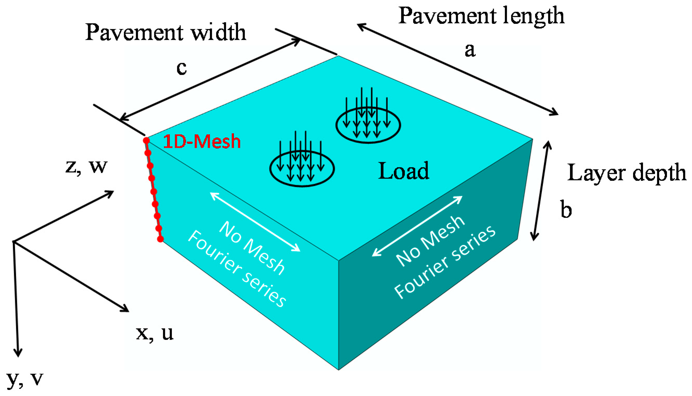
The finite layer method (FLM) is proposed as another alternative way for analyzing the structural response of pavements, whilst reducing the computational requirements without decreasing the computational accuracy. This method combines a one-dimensional (1D) FEM discretization in the pavement depth direction with Fourier series in the two horizontal directions, which can be considered as a further development of the semi-analytical FEM. The idea is particularly suitable for multilayered structures. Furthermore, due to the use of Fourier series in two directions, the computational cost of FLM is significantly lower than that of conventional FE analysis methods. The FLM started to be applied in the analysis of elastic, horizontally layered foundations from 1979 [20], when the basic theory and application were proposed. Thereafter, the approach was further developed for the analysis of nonhomogeneous soils whose modulus increases linearly with depth [21]. An exact finite layer flexibility matrix was introduced to overcome the difficulties when the conventional finite layer stiffness approach was applied to incompressible materials [22,23]. Meanwhile, soil consolidation and surface deformation entailing the extraction of water was also investigated by using this approach [24,25,26]. In the next several years, researchers applied the FLM in groundwater flow models [27] and analyses of 3D Biot consolidation of layered transversely isotropic soils [28]. Recently, the FLM was applied for modeling the noise transmission through double walls [29]. analytical model, called 3D-Move uses a continuum-based FLM to compute pavement responses [30,31]. The 3D-Move model can account for important pavement response factors such as moving loads, 3D contact stress distributions (normal and shear) of any shape, and viscoelastic material characterization for the pavement layers.

Although the 3D-Move is freely available, it is not open source, and it still lacks some specific features such as the interlayer behavior for the pavement modeling. Therefore, a re-implementation of the FLM in code is necessary. As mentioned in the manual of 3D-Move, the accuracy of the calculated results is not guaranteed. Therefore, an algorithm or a technique that can provide more accurate results is of significant importance. In recent years, the research on super-convergence has increasingly drawn attention since it can provide higher order accuracy. A number of research studies have been conducted on this subject [32,33]. In recent years, a super-convergence technique named Element Energy Projection (EEP) method was proposed by Yuan et al. [34,35,36]. Its core assumption is to assume the energy projection theorem in the FEM mathematical theory [37] to be almost true for a single element. For various 1D problems, this assumption proves to be true and the convergent displacements and derivatives of the simplified form (i.e., with linear test/weight functions) converge at least one order higher than the conventional FEM results [38]. This method has been proven to be simple, convenient and effective. Moreover, it can be easily applied to other specific FE methods including FLM.

In the following sections, the basic theory of FLM is introduced, based on which the computer code named EasyFEM is self-developed. The EEP super-convergence strategy for EasyFEM is then described in detail to improve the accuracy of the results derived from EasyFEM. The EasyFEM is verified by comparing the results from BISAR and ABAQUS; the convergence rates between the results from ordinary EasyFEM and the EasyFEM with the post-processing with EEP are compared. The application of EasyFEM is to predict the mechanical responses of asphalt pavements. Lastly, a brief summary and outlook are provided.

2. Numerical Solution of EasyFEM

2.1. Finite Elements

A typical 3D EasyFEM model for the pavement problem was set up as shown in Figure 1.

The system is discretized in the pavement depth direction; thus, the conventional 1D isoparametric elements of degree k can be adopted, e.g., the 3-node quadratic elements as shown in Figure 2:

Figure 2. The natural coordinates for 1D quadratic elements.

Figure 2. The natural coordinates for 1D quadratic elements.

where the shape function used was as follows:

$$\begin{gathered} N_1=\frac{-\xi \left(1-\xi \right)}{2} \\ {N}_2=\frac{\xi \left(1+\xi \right)}{2} \\ {N}_3=1-{\xi }^2 \end{gathered}$$

(1)

with $\xi$ being local coordinate.

2.2. FE Solution of Displacements

The pavement is assumed to be supported at side edges (x = 0, x = a, z = 0 and z = c) in a manner preventing all displacements in the vertical planes but permitting “unrestricted” movement in the x- and z-directions. The shape functions are re-written as the conventional 1D shape functions multiplied by the Fourier series, in which x ranges between zero and a; z ranges between zero and c. If the displacement functions with three components u, v and w are formulated in the following form, the boundary condition will meet this above-mentioned requirement:

$$\begin{gathered} d=\{\begin{array}{c}u\\ v\\ w\end{array}\}={\displaystyle \sum }_{m=1}^M{\displaystyle \sum }_{n=1}^N\left[\begin{array}{ccc}cos\frac{m\pi x}{a}sin\frac{n\pi z}{c}& 0& 0\\ 0& sin\frac{m\pi x}{a}sin\frac{n\pi z}{c}& 0\\ 0& 0& sin\frac{m\pi x}{a}cos\frac{n\pi z}{c}\end{array}\right]\{\begin{array}{c}{u}^{mn}\\ v^{mn}\\ w^{mn}\end{array}\} \\ ={\sum }_{m=1}^M{\sum }_{n=1}^N{N}^{mn}·d^{mn}, \\ \mathrm{with}{N}^{mn}=\left[\begin{array}{ccc}cos\frac{m\pi x}{a}sin\frac{n\pi z}{c}& 0& 0\\ 0& sin\frac{m\pi x}{a}sin\frac{n\pi z}{c}& 0\\ 0& 0& sin\frac{m\pi x}{a}cos\frac{n\pi z}{c}\end{array}\right], d^{mn}=\{\begin{array}{c}{u}^{mn}\\ v^{mn}\\ w^{mn}\end{array}\}=\left[N_k\left(y\right)\right]\left\{d_k^{mn}\right\}. \end{gathered}$$

(2)

$N^{mn}$ is the matrix for the Fourier series expansion in the two horizontal directions, $d^{mn}$ is the displacement vector without the Fourier series expansion, $\left[N_k\left(y\right)\right]$ is the conventional 1D shape function applied in the FEM model, and $\left\{d_k^{mn}\right\}$ represents the corresponding nodal displacements.

Similarly, the loading function for the pavement analysis can be formulated as:

$$\begin{gathered} f={\displaystyle \sum }_{m=1}^M{\displaystyle \sum }_{n=1}^{N}p\left(y\right)sin\frac{m\pi x}{a}sin\frac{n\pi z}{c}={\displaystyle \sum }_{m=1}^M{\displaystyle \sum }_{n=1}^N{\left\{p\right\}}^{mn}, \\ p\left(y\right)={{\displaystyle \sum }}_{s=1}^S\left(\frac{2P_s}{m\pi }\right)\left[cos\frac{m\pi }{a}{X}_{s1}-cos\frac{m\pi }{a}{X}_{s2}\right]{{\displaystyle \sum }}_{t=1}^T\left(\frac{2P_t}{n\pi }\right)\left[cos\frac{n\pi }{c}{Z}_{t1}-cos\frac{n\pi }{c}{Z}_{t2}\right], \end{gathered}$$

(3)

where m and n are the terms of Fourier series in the x and z directions, respectively. In this study, both M and N are adopted as 100, which has been previously proved to be sufficiently accurate to represent the load variation [16,17]. The product of P_s and P_t represents the tire load pressure, when m = n; X_s1 and Z_t1 are the x and z coordinates, where the tire load area starts, respectively; X_s2 and Z_t2 are the x and z coordinates where the tire load area ends, respectively.

At the nodes the strains are determined through displacements:

$$\begin{array}{l}\epsilon =\{\begin{array}{c}{\epsilon }_x\\ {\epsilon }_y\\ {\epsilon }_z\\ {\gamma }_{xy}\\ {\gamma }_{yz}\\ {\gamma }_{zx}\end{array}\}=\left[\begin{array}{c}\begin{array}{ccc}\frac{\partial }{\partial x}& 0& 0\\ 0& \frac{\partial }{\partial y}& 0\\ 0& 0& \frac{\partial }{\partial z}\end{array}\\ \begin{array}{ccc}\frac{\partial }{\partial y}& \frac{\partial }{\partial x}& 0\\ 0& \frac{\partial }{\partial z}& \frac{\partial }{\partial y}\\ \frac{\partial }{\partial z}& 0& \frac{\partial }{\partial x}\end{array}\end{array}\right]d =\left(L_1\frac{\partial }{\partial x}+L_2\frac{\partial }{\partial y}+L_3\frac{\partial }{\partial z}\right){\displaystyle {\displaystyle \sum }_{m=1}^M}{\displaystyle {\displaystyle \sum }_{n=1}^N}{N}^{mn}·d^{mn}\\ ={\sum }_{m=1}^M{\sum }_{n=1}^N{E}^{mn}{d}^{mn}= {\sum }_{m=1}^M{\sum }_{n=1}^N{B}^{mn}·\left\{d_k^{mn}\right\},\end{array}$$

(4)

where L₁, L₂, L₃ are three different matrices of size 6 × 3 whose elements are either 0 or 1,

$$E^{mn}=L_1\frac{\partial N^{mn}}{\partial x}+L_2{N}^{mn}\frac{\partial }{\partial y}+L_3\frac{\partial N^{mn}}{\partial z},$$

(5)

and matrix

$$B^{mn}=\left[B_1^{mn}{B}_2^{mn}\cdots B_{k+1}^{mn}\right]=\left[\begin{array}{ccc}{E}^{mn}{N}_1\left(y\right)& E^{mn}{N}_2\left(y\right)& \cdots E^{mn}{N}_{k+1}\left(y\right)\end{array}\right]$$

(6)

is called the strain-displacement matrix.

The relation between stresses and strains is used to express the total potential energy with nodal displacements $\left\{d\right\}$:

$$\Pi \left(\left\{d\right\}\right)={{\displaystyle \int }}_V^{}\frac{1}{2}{\left(\left[B\right]\left\{d\right\}\right)}^T\left[D\right]\left(\left[B\right]\left\{d\right\}\right)dV-{{\displaystyle \int }}_V^{}{\left(\left[N\right]\left\{d\right\}\right)}^T\left\{b\right\}dV-{{\displaystyle \int }}_S^{}{\left(\left[N\right]\left\{d\right\}\right)}^T\left\{f\right\}dS .$$

(7)

The nodal displacements $\left\{d\right\}$ which correspond to the minimum of the functional $\Pi$ are determined by the condition that the first variation of $\Pi$ should be zero, i.e.,

$$\begin{gathered} \delta \Pi \left(\left\{d\right\}\right)=0, \\ \delta \Pi \left(\left\{d\right\}\right)={\int }_V{\left\{\delta d\right\}}^T{\left[B\right]}^T\left[D\right]\left[B\right]\left\{d\right\}dV-{\int }_V{\left\{\delta d\right\}}^T{\left[N\right]}^T\left\{b\right\}dV-{\int }_S{\left\{\delta d\right\}}^T{\left[N\right]}^T\left\{f\right\}dS . \end{gathered}$$

(8)

Then, the arbitrariness of $\left\{\delta d\right\}$ leads the following equilibrium equation for FE:

$${{\displaystyle \int }}_V{\left[B\right]}^T\left[D\right]\left[B\right]dV\left\{d\right\}-{{\displaystyle \int }}_V{\left[N\right]}^T\left\{b\right\}dV-{{\displaystyle \int }}_S{\left[N\right]}^T\left\{f\right\}dS =0,$$

(9)

which is commonly given in the following form:

$$\begin{gathered} \left[k\right]\left\{d\right\}=\left\{f\right\}, \\ \left[k\right]={\int }_V{\left[B\right]}^T\left[D\right]\left[B\right]dV\mathrm{and}\left\{f\right\}={\int }_V{\left[N\right]}^T\left\{b\right\}dV+{\int }_S{\left[N\right]}^T\left\{f\right\}dS, \end{gathered}$$

(10)

where [k] is the element stiffness matrix; and $\left\{f\right\}$ is the load vector.

From Equations (4) and (10), the stiffness matrix of one element includes:

$$\begin{gathered} I_1={{\displaystyle \int }}_0^a{{\displaystyle \int }}_0^c\sin \frac{m\pi x}{a}\sin \frac{n\pi z}{c}·\sin \frac{p\pi x}{a}\sin \frac{q\pi z}{c}·dxdz, \\ {I}_2={{\displaystyle \int }}_0^a{{\displaystyle \int }}_0^c\cos \frac{m\pi x}{a}\sin \frac{n\pi z}{c}·\cos \frac{p\pi x}{a}\sin \frac{q\pi z}{c}·dxdz, \\ {I}_3={{\displaystyle \int }}_0^a{{\displaystyle \int }}_0^c\cos \frac{m\pi x}{a}\cos \frac{n\pi z}{c}·\cos \frac{p\pi x}{a}\cos \frac{q\pi z}{c}·dxdz. \end{gathered}$$

(11)

The integrals exhibit orthogonal properties, which ensure that:

$$I_1=I_2=I_3=\left\{\begin{array}{c}\frac{ac}{4}, for m=p and n=q\\ 0,for m\ne p or n\ne q\end{array}\right\}.$$

(12)

This means that the matrix ${\left(k^{mnpq}\right)}^{\mathrm{e}}$ is diagonal. In other words, the non-zero values are only located on the diagonal, where m = p and n = q. Thus, the stiffness matrix can be reduced to:

$${\left(k_{gk}^{mnmn}\right)}^e=\frac{ac}{4}{\int }_{length}\left({B_g^{mn}}^{T}D{B}_k^{mn}\right)dym=1, 2\dots M; n=1,2\dots N,$$

(13)

where g and k represent the nodes of the element, respectively. The length corresponds to the length of the element.

A typical term for the force vector becomes:

$${\left(f^{mn}\right)}^e={\int \int \int }_{vol}{\left(N^{mn}\right)}^T{\left\{p\right\}}^{mn}dxdydz.$$

(14)

By assembling the stiffness matrix of each element to the global domain, the global linear system is achieved as follows:

$$\left[\begin{array}{cccc}{K}^{1111}& & & \\ & K^{1212}& & \\ & & \ddots & \\ & & & K^{MNMN}\end{array}\right]\left\{\begin{array}{c}{U}^{11}\\ U^{12}\\ ⋮\\ U^{MN}\end{array}\right\}+\left\{\begin{array}{c}{F}^{11}\\ F^{12}\\ ⋮\\ F^{MN}\end{array}\right\}=0.$$

(15)

Equation (15) shows that the large system of equations splits up into $M\times N$ separate problems:

$$K^{mnmn}{U}^{mn}+F^{mn}=0,$$

(16)

where K is the global stiffness matrix; U is the global displacement vector; and F is the global loading vector.

3. EEP Super-Convergence Strategy for EasyFEM

When Equation (16) is solved for $U^{mn}$, both $d^{mn}$ and $d$ can be obtained from Equation (2). These two approximate solutions are denoted as $d_h^{mn}$ and $d_h$ to distinguish them from the exact solutions. It is clear, that if M and N are fixed, the accuracy of $d_h$ mainly depends on the accuracy of$d_h^{mn}$. For conventional FEM models, a rather extensive mesh should be used to attain more accurate $d_h^{mn}$, which leads to a large number of degrees of freedom in the calculation. In this case, the newly-developed super-convergence technique EEP was introduced into EasyFEM as to improve the accuracy of the solutions for strains and stresses over the whole pavement model.

The original idea of the EEP technique came from a well-known mathematical theorem for FEM called the projection theorem [37]. Actually, the principle of minimum potential energy with respect to nodal displacements $\left\{d\right\}$ in Equation (8) can be rewritten in the same manner with respect to the continuous 1D displacement $d\left(y\right)$ as follows:

$$\delta \mathsf{\Pi }\left(d\left(y\right)\right)={\int }_V\delta d{\left(y\right)}^T{\left[E\right]}^T\left[D\right]\left[E\right]d\left(y\right)dV-{\int }_V\delta d{\left(y\right)}^T{\left[N\left(x,z\right)\right]}^T\left\{b\right\}dV-{\int }_S\delta d{\left(y\right)}^T{\left[N\left(x,z\right)\right]}^T\left\{f\right\}dS =0.$$

(17)

By replacing $\delta d\left(y\right)$ in Equation (17) with the test displacement $\tilde{d}\left(y\right)$, an equivalent expression for the above principle of minimum potential energy is the virtual work equation as follows:

$$\begin{gathered} a(d\left(y\right),\tilde{d}\left(y\right))=(f,\tilde{d}\left(y\right)),\forall \tilde{d}\left(y\right)\in S^h, \\ \mathrm{with}a\left(d\left(y\right),\tilde{d}\left(y\right)\right)={\int }_V\tilde{d}{\left(y\right)}^T{\left[E\right]}^T\left[D\right]\left[E\right]d\left(y\right)dV， \\ (\mathrm{f},\tilde{\mathrm{d}}\left(\mathrm{y}\right))={\int }_{\mathrm{V}}\tilde{\mathrm{d}}{\left(\mathrm{y}\right)}^{\mathrm{T}}{\left[\mathrm{N}\left(\mathrm{x},\mathrm{z}\right)\right]}^{\mathrm{T}}\left\{\mathrm{b}\right\}\mathrm{dV}+{\int }_{\mathrm{S}}\tilde{\mathrm{d}}{\left(\mathrm{y}\right)}^{\mathrm{T}}{\left[\mathrm{N}\left(\mathrm{x},\mathrm{z}\right)\right]}^{\mathrm{T}}\left\{\mathrm{f}\right\}\mathrm{dS}, \end{gathered}$$

(18)

where $a\left(·,·\right)$ and $\left(·,·\right)$ are defined as the energy product and the linear form in mathematics, respectively, and $S^h$ is the test space of FLM.

It can be easily understood that Equation (18) holds true both for the exact solution $d\left(y\right)$ and the approximate solution $d_h\left(y\right)$. Always taking the same test displacement for these two cases, the following projection theorem is derived for FLM:

$$a(d\left(y\right)-d_h\left(y\right),\tilde{d}\left(y\right))=0,\forall \tilde{d}\left(y\right)\in S^h.$$

(19)

This theorem holds true over the entire 3D pavement model. By assuming that it is approximately true over one element of FLM, the EEP equation was obtained:

$$a^e(d\left(y\right)-d_h\left(y\right),\tilde{d}\left(y\right))\approx 0,\forall \tilde{d}\left(y\right)\in S^h.$$

(20)

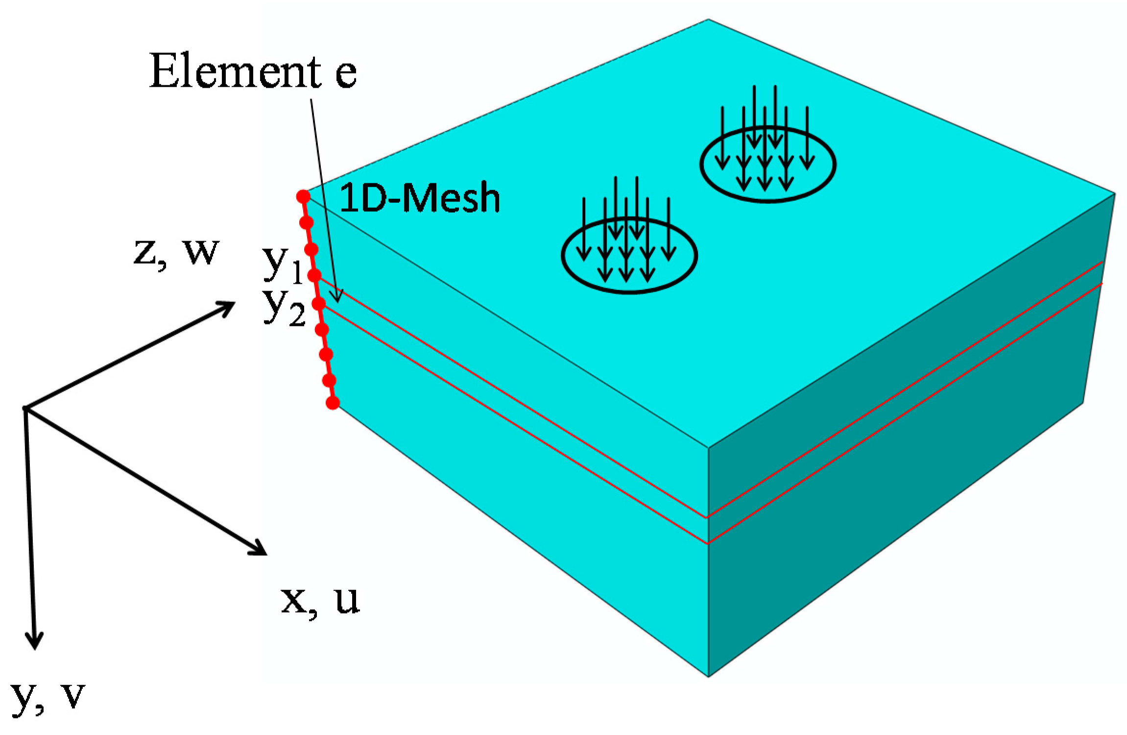
A typical element e of the FLM is shown in Figure 3, which is actually a small layer of the pavement with the y-coordinate ranging from y₁ to y₂.

Denote $e_h=d\left(y\right)-d_h\left(y\right)$. Then:

$$\begin{array}{l}{a}^e\left(d\left(y\right)-d_h\left(y\right),\tilde{d}\left(y\right)\right)={{\displaystyle \int }}_{V_e}\tilde{d}{\left(y\right)}^T{\left[E\right]}^T\left[D\right]\left[E\right]e_{h}dV\\ ={\sum }_{m=1}^M{\sum }_{n=1}^N{\int }_{V_e}{{\tilde{d}}^{mn}}^T{\left[E^{mn}\right]}^T\left[D\right]\left[E^{mn}\right]e_h^{mn}dV={\sum }_{m=1}^M{\sum }_{n=1}^N{a}^e(e_h^{mn},{\tilde{d}}^{mn})\approx 0.\end{array}$$

(21)

Denoting $E_{13}^{mn}=L_1\frac{\partial N^{mn}}{\partial x}+L_3\frac{\partial N^{mn}}{\partial z}$, $E_2^{mn}=L_2{N}^{mn}$, and considering the zeros from integration of the Fourier series as shown in Equation (12), Equation (21) can be further rewritten as follows:

$$\begin{array}{l}{\sum }_{m=1}^M{\sum }_{n=1}^N{\int }_{V_e}^{}{\left(E_{13}^{mn}{\tilde{d}}^{mn}+E_2^{mn}\frac{\partial {\tilde{d}}^{mn}}{\partial y}\right)}^T\left[D\right]\left(E_{13}^{mn}{e}_h^{mn}+E_2^{mn}\frac{\partial e_h^{mn}}{\partial y}\right)dV=\\ {\sum }_{m=1}^M{\sum }_{n=1}^N{\int }_{y_1}^{y_2}[{\left(\frac{\partial {\tilde{d}}^{mn}}{\partial y}\right)}^T{A}^{mn}\frac{\partial e_h^{mn}}{\partial y}+{\left(\frac{\partial {\tilde{d}}^{mn}}{\partial y}\right)}^T{G}^{mn}{e}_h^{mn}+{\left({\tilde{d}}^{mn}\right)}^T{\left(G^{mn}\right)}^T\frac{\partial e_h^{mn}}{\partial y}+\\ {\left({\tilde{d}}^{mn}\right)}^T{H}^{mn}{e}_h^{mn}]dy\approx 0,\end{array}$$

(22)

where

• $A^{mn}={\int }_0^a{\int }_0^c{\left(E_2^{mn}\right)}^T\left[D\right]E_2^{mn}dxdz,$
• $G^{mn}={\int }_0^a{\int }_0^c{\left(E_2^{mn}\right)}^T\left[D\right]E_{13}^{mn}dxdz,$
• $H^{mn}={\int }_0^a{\int }_0^c{\left(E_{13}^{mn}\right)}^T\left[D\right]E_{13}^{mn}dxdz,$

with integration by parts along the y-direction, the EEP can be equivalently converted into the following expression:

$${\displaystyle \sum }_{m=1}^M{\displaystyle \sum }_{n=1}^N{{\displaystyle \int }}_{y_1}^{y_2}\left(-{{\tilde{d}}^{mn}}^T{A}^{mn}\frac{{\partial }^2{e}_h^{mn}}{\partial y^2}+{{\tilde{d}}^{mn}}^T({\left(G^{mn}\right)}^T-G^{mn})\frac{\partial e_h^{mn}}{\partial y}+{\left({\tilde{d}}^{mn}\right)}^T{H}^{mn}{e}_h^{mn}\right)dy+{\left({{\tilde{d}}^{mn}}^T(A^{mn}\frac{\partial e_h^{mn}}{\partial y}+G^{mn}{e}_h^{mn})\right)}_{y_1}^{y_2}\approx 0.$$

(23)

Since the test function ${\tilde{d}}^{mn}$ can be arbitrarily selected for any m and n, the left side of Equation (23) is decoupled into

$${\int }_{y_1}^{y_2}{{\tilde{d}}^{mn}}^T\left(-A^{mn}\frac{{\partial }^2{e}_h^{mn}}{\partial y^2}+\left({G^{mn}}^T-G^{mn}\right)\frac{\partial e_h^{mn}}{\partial y}+H^{mn}{e}_h^{mn}\right)dy+{\left({{\tilde{d}}^{mn}}^T(A^{mn}\frac{\partial e_h^{mn}}{\partial y}+G^{mn}{e}_h^{mn})\right)}_{y_1}^{y_2}\approx 0.$$

(24)

Taking two linear polynomials:

$${\overline{N}}_1=\frac{y_2-y}{y_2-y_1}; {\overline{N}}_2=\frac{y-y_1}{y_2-y_1}$$

(25)

as two test functions ${\tilde{d}}^{mn}$, respectively, and considering that:

$$d^{mn}\left(y_1\right)=d_h^{mn}\left(y_1\right),d^{mn}\left(y_2\right)=d_h^{mn}\left(y_2\right),$$

(26)

since the nodal displacements are super-convergent based on mathematical theory, one can obtain the following equation to calculate a recovered derivative solution at either of the two end-nodes of element e [39]:

$$\begin{array}{lll}\frac{\partial d_E^{mn}\left(y_1\right)}{\partial y}& =& {\left(A^{mn}\right)}^{-1}\left[\left(b,{\overline{N}}_1\right)-a^e\left(d_h^{mn},{\overline{N}}_1\right)-G_1{d}_h^{mn}\left(y_1\right)\right],\\ \frac{\partial d_E^{mn}\left(y_2\right)}{\partial y}& =& -{\left(A^{mn}\right)}^{-1}\left[\left(b,{\overline{N}}_2\right)-a^e\left(d_h^{mn},{\overline{N}}_2\right)+G_2{d}_h^{mn}\left(y_2\right)\right],\end{array}$$

(27)

where:

$$i=1,2,m=1,\cdots ,M,n=1,\cdots ,N.$$

(28)

Substituting the derivative results calculated from Equation (28) into Equation (4), recovered strains and the corresponding stresses are obtained for the pavement model. This is the EEP super-convergence technique for FLM. When it is implemented in EasyFEM, stresses are obtained with much fewer elements and significantly less computational effort.

4. Numerical Analysis Using EasyFEM and EEP Techniques

4.1. Analytical Verification of EasyFEM

The analytical verification of the EasyFEM without EEP post-processing was carried out. The models of the asphalt pavement were created in BISAR, ABAQUS and EasyFEM, which are representative software applications developed based on LET, FEM and FLM, respectively. The pavement type is widely used in Germany according to the guidelines RStO-12 [40] and RDO-Asphalt-09 [1], as shown in Figure 4. 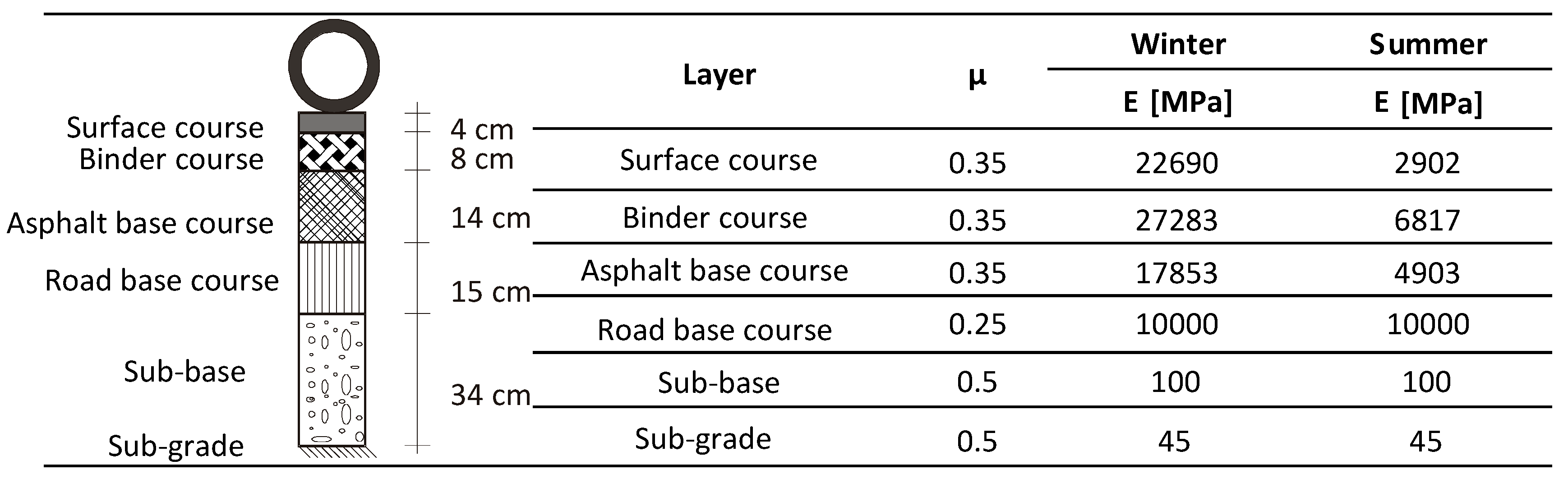The thicknesses of all layers except for the sub-grade were derived from RstO-12 [40]. The thickness of the sub-grade was defined to be 2000 mm in ABAQUS and EasyFEM after a previous mesh study in order to minimize the influence of the boundary on the computational results. Furthermore, the length and width of the pavement in the full-scale model were set to be 6000 mm based on the same reason. A full-scale model was created in the EasyFEM while the model in ABAQUS was one-fourth symmetrical model. The full-scale model exhibits advantages for the simulation of nonsymmetrical models with complex loading conditions in the further development of the EasyFEM. In BISAR, the thickness of the sub-grade as well as the length and width of the pavement were set to be infinite according to the LET. The pavement surface temperatures of −12.5 (winter) and 27.5 °C (summer) were assumed, and then the associated material properties were determined according to RDO-Asphalt-09 [1], as listed in Figure 4.

The square load with the side length of 264 mm and uniformly distributed contact stress of 0.7 MPa was applied at the center of the full-scale pavement surface in the EasyFEM and a corresponding set-up was applied in ABAQUS. In BISAR, only circular loads can be defined and thus a uniform contact load of 0.7 MPa with a radius of 150 mm was applied. In all models, the three asphalt layers were totally bound; the two contact layers among the asphalt base course, road base course, sub-base and sub-grade were defined as being partially bound.

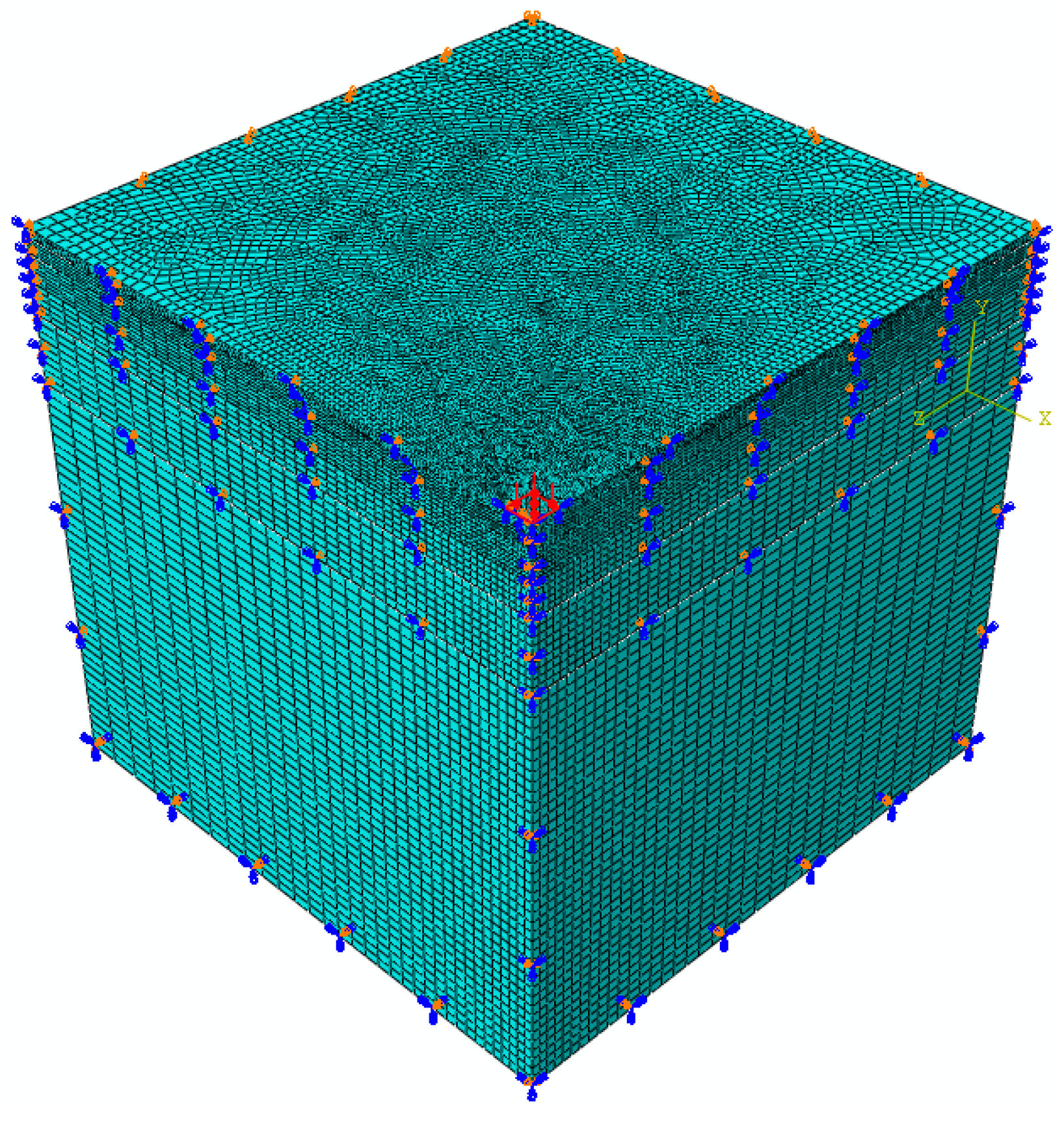
In order to attain a high accuracy, a very fine mesh was adopted in ABAQUS and EasyFEM after a mesh study. The mesh size in EasyFEM was uniformly set as 10 mm and thus 275 3-node quadratic elements with 551 nodes were generated. In order to reduce the computational consumption, the mesh size increases gradually from the top to the bottom and from the loading center to the boundary in the one-fourth symmetrical model in ABAQUS, as shown in Figure 5. The number of elements and nodes in ABAQUS are 162,728 and 193,601, respectively. There was no mesh generated from the BISAR.

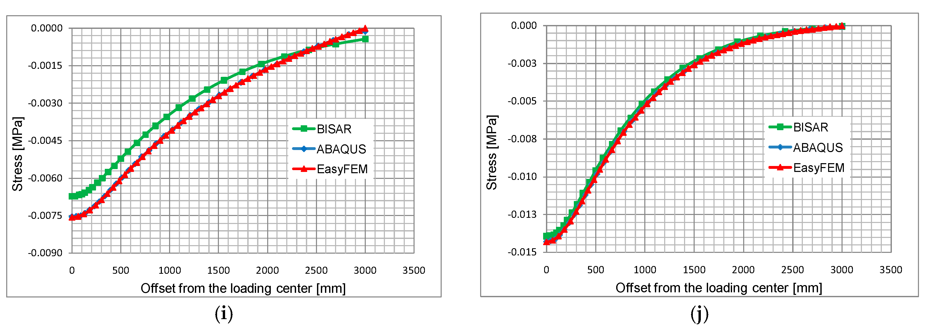
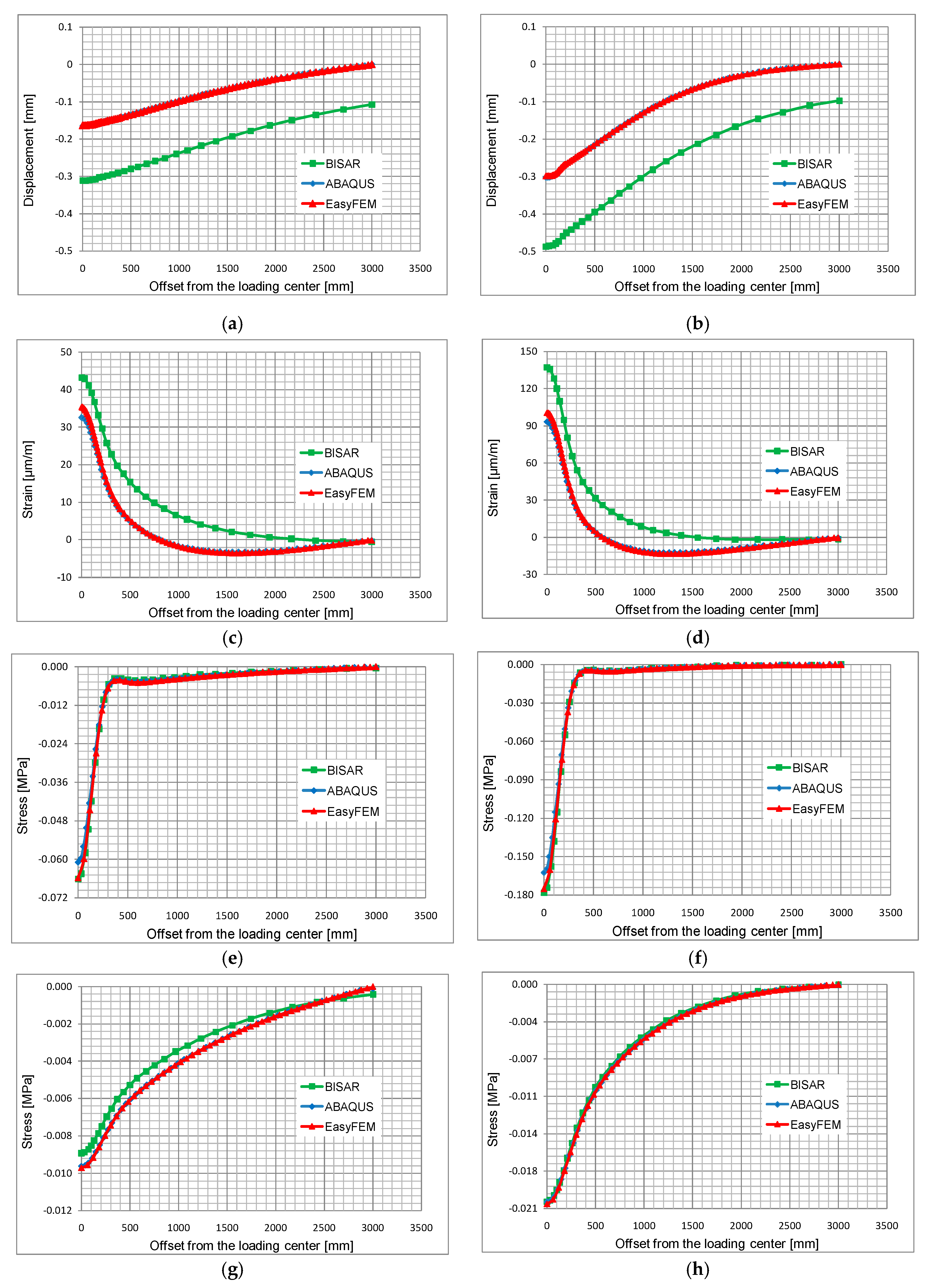
The computational results shown in Figure 6 are derived from five series of response points offset from the loading center to the boundary.

Given these figures, it can be concluded that the results derived from ABAQUS and EasyFEM are consistent with each other, yet the results from BISAR exhibit great deviations from those from the other two software applications, especially along the first two series of response points. The underlying reasons for the differences can be attributed to the different geometrical definitions of the models in BISAR due to its intrinsic limitation (circular load, infinite length and width of the layers and infinite thickness of the sub-grade); the deviations are the largest at the response points that are closest to the load.

In

Table 1. Comparison between ABAQUS and EasyFEM based on the results at critical points below the loading center.

Points	Results	Winter
		EasyFEM	ABAQUS	Difference
1	Vertical displacement [mm]	−1.63 × 10−1	−1.64 × 10−1	7.72 × 10−4 (−0.47%)
2	Horizontal strain [-]	3.54 × 10−5	3.25 × 10−5	2.82 × 10−6 (8.68%)
3	Vertical stress [MPa]	−6.57 × 10−2	−6.09 × 10−2	−4.84 × 10−3 (7.95%)
4	Vertical stress [MPa]	−9.70 × 10−3	−9.62 × 10−3	−8.61 × 10−5 (0.90%)
5	Vertical stress [MPa]	−7.57 × 10−3	−7.55 × 10−3	−1.51 × 10−5 (0.20%)
Points	Results	Summer
		EasyFEM	ABAQUS	Difference
1	Vertical displacement [mm]	−2.99 × 10−1	−3.02 × 10−1	3.24 × 10−3 (−1.07%)
2	Horizontal strain [-]	1.01 × 10−4	9.33 × 10−5	7.39 × 10−6 (7.92%)
3	Vertical stress [MPa]	−1.75 × 10−1	−1.62 × 10−1	−1.27 × 10−2 (7.85%)
4	Vertical stress [MPa]	−2.06 × 10−2	−2.04 × 10−2	−1.75 × 10−4 (0.86%)
5	Vertical stress [MPa]	−1.43 × 10−2	−1.43 × 10−2	−1.01 × 10−5 (0.07%)

, the computational results from ABAQUS and EasyFEM are considered at five critical locations directly below the loading center shown in Figure 6, where maximum compressive or tensile values may occur.

It can be stated that the results from both programs have a high correlation except for a slightly larger difference in the horizontal strain at the bottom of the asphalt base course and vertical stresses at the top of the sub-base. Considering the different element types and mesh algorithms in the two programs, the differences are judged to be acceptable. Moreover, the computational time of the EasyFEM is much shorter than that of the ABAQUS. Both analyses were run on a computer with an Intel Core Duo 3.4 GHz, 32 GB RAM (Santa Clara, CA, USA). On average, the computational time required by the ABAQUS is about 420 s, whereas the EasyFEM model requires 120 s. It is worth mentioning that the model in ABAQUS is one-fourth symmetrical, but the one in EasyFEM is full-scale. With code optimization, the computation time of the EasyFEM can be reduced further. In summary, the accuracy and efficiency of the EasyFEM are proved by these comparisons.

4.2. Comparison of Convergence Rate between Ordinary EasyFEM and EasyFEM with EEP Post-Processing Techniques

As discussed above, by using 275 3-node quadratic finite elements along the y-direction, EasyFEM has performed fairly well compared to ABAQUS. If the number of elements can be further reduced without decreasing the computational accuracy, the EasyFEM will be even more suitable for application in pavement design and assessment from an engineering point of view. The EEP technique for recovering derivatives makes this possible. The convergence rates between ordinary EasyFEM and EasyFEM with the EEP post-processing technique are compared in this section to show the impact of the EEP technique on the solution accuracy.

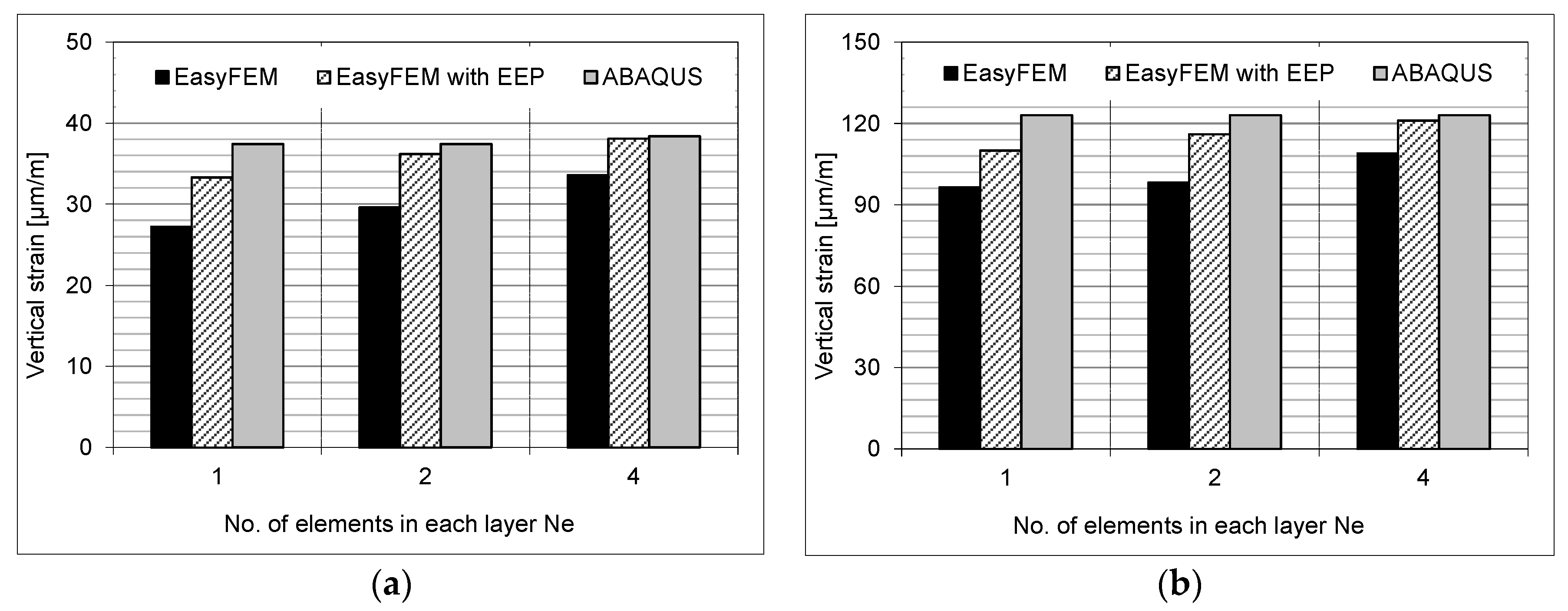
To emphasize the significant improvement brought about by the application of EEP, a series of rough meshes with 2-node linear elements was adopted in the EasyFEM. In particular, three models with different meshes were created, i.e., each layer of the asphalt pavement was divided into one, two and four elements (N_e = 1, 2 and 4), respectively; the asphalt pavement had six layers resulting in a total of 6 × N_e = 6, 12 and 24 linear elements in the three pavement models. EasyFEM with the EEP post-processing technique can produce strains and stresses with a higher accuracy, which is demonstrated by a number of numerical results. In Figure 7, vertical strains at the points located below the loading center and at the bottom of asphalt base course were compared between ordinary EasyFEM and EasyFEM with the EEP technique, where one, two and four linear finite elements were used in each layer along the y-direction, respectively. The results from the model with the fine mesh in ABAQUS created in Section 4.1 were taken as the reference. Since the stresses are calculated by multiplying strains with elastic constants, similar results can be obtained for vertical stresses as well. It can be seen that the EEP technique for FLM, which converges faster, can significantly improve the accuracy of vertical strains and stresses of a plain EasyFEM. With the EEP technique, the EasyFEM can offer reliable results much more quickly and efficiently and is thus suitable to be applied in pavement engineering practice.

4.3. Application of EasyFEM

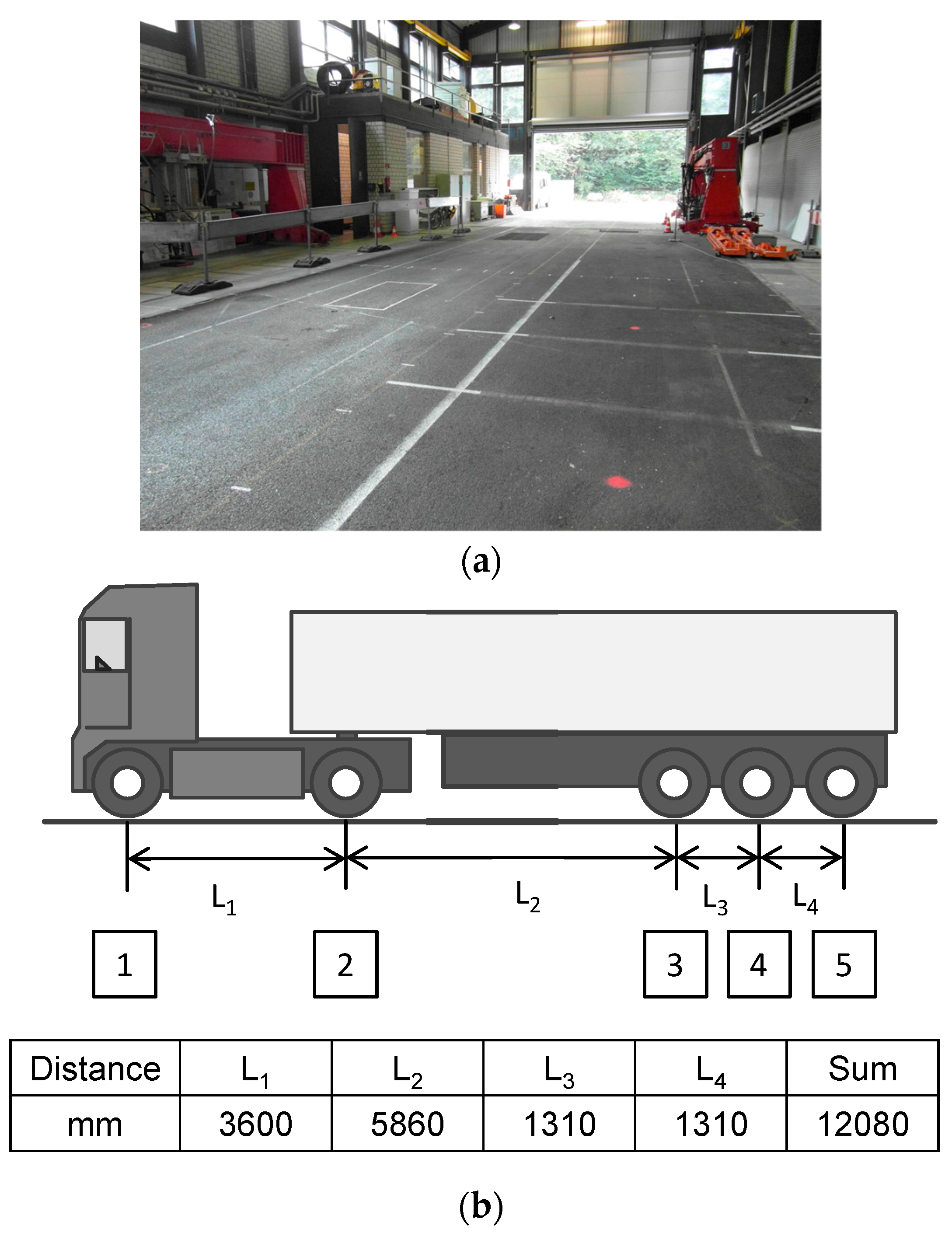
The EasyFEM was used to predict the mechanical responses and the predictions were compared with the data derived from field measurements on the test track of the German Federal Highway Research Institute (BASt), as shown in Figure 8a. A truck driving at a speed of approximately 30 km/h was selected for the measurement to apply the loads, as shown in Figure 8b.

During the test track construction, strain gauges and pressure load cells were embedded at different depths of the test track along the center of the wheel path, which can measure strains and stresses along the corresponding directions when the truck passes. Due to the low speed of loads and the suggestion from [17], a static analysis with stationary loads is precise enough to compute the pavement responses. The material parameters of the pavement layers were derived from the laboratory tests on the specimens drilled from the test track. The thicknesses and the material properties of the test track are listed in

Table 2. Layer thickness and material properties of the test track.

Layer	Thickness [mm]	µ	E [MPa]
Surface course	40	0.35	11150
Binder course	50	0.35	10435
Asphalt base course	110	0.35	6893
Gravel base layer	150	0.49	157.8
Frost protection layer	570	0.49	125.7
Sub-grade	2000	0.49	98.9

[17]. The length longitudinal to the direction of traffic (both directions) was defined as 20 times the loading radius to limit the time required for the computational calculation. The width of the pavement was defined to be 3750 mm.

The loading parameters are listed in

Table 3. Loading parameters of the tire.

Axle	Wheel Number	Pressure [MPa]	Axle Load [kg]
1	2	0.522	7425
2	4	0.377	10725
3	2	0.513	7300
4	2	0.511	7275
5	2	0.519	7375

[17]. All of the contact areas are assumed as squares with a side length of 264 mm. The distance between the center of the first left tire and the left edge of the test track along the traffic direction is 1100 mm.

The upper three asphalt layers were totally bound. The two contact layers between the asphalt base course, gravel base layer, frost protection layer and sub-grade were defined as being partially bound. The 3-node quadratic elements with the mesh size of 10 mm were applied in the EasyFEM with the EEP technique.

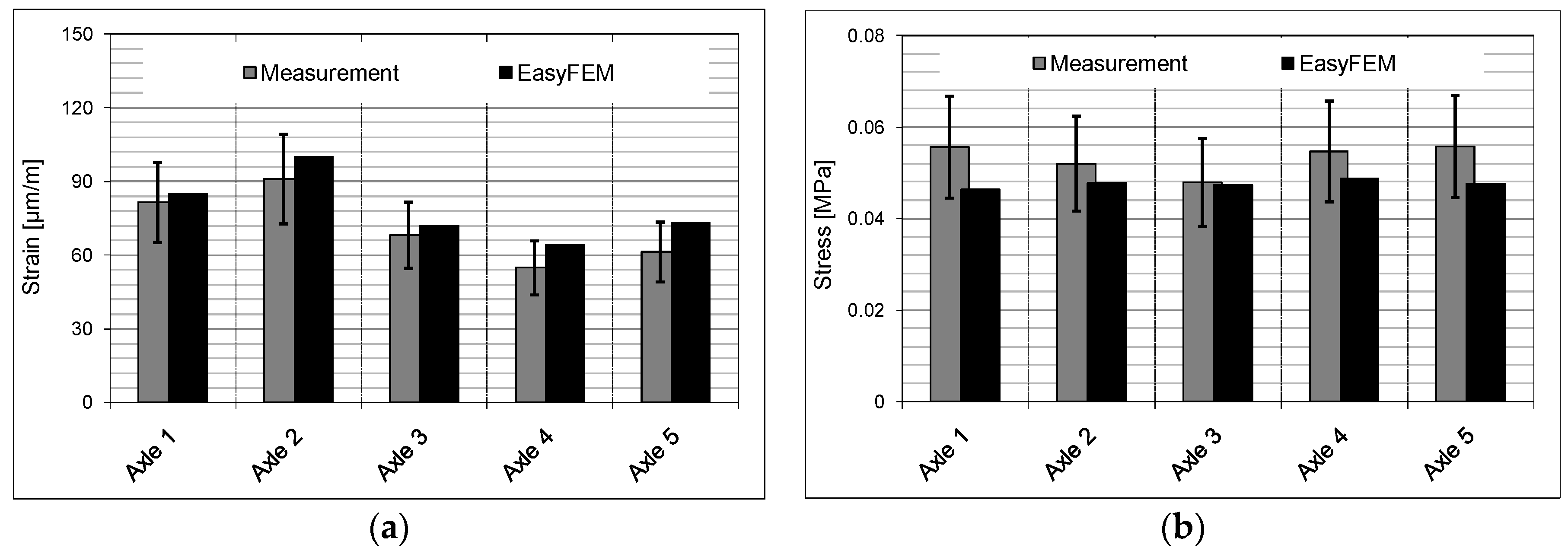
The following computational values were compared with the measured data, which is used to verify the EasyFEM. The strain along the traffic direction at the bottom of the asphalt base course and the vertical tensile stress at the top of the gravel base layer from the location below the center of the left tire of each axle were used in the validation process. The values from the measurement and simulation can be seen in Figure 9. All computational strains are higher than the measured values and all computational stresses are lower than those obtained from the measurements. Due to the uncertainties and fluctuations, the error range is considered to be ±20% [17]. The computational values are all within this range. Thus, the EasyFEM is suited to simulate the response of the asphalt pavement under the traffic load with sufficient accuracy.

5. Conclusions

Initially, the EasyFEM code is developed to predict the mechanical responses of asphalt pavements under stationary load. The accuracy of the program is verified by comparing the results to those obtained from BISAR and ABAQUS. The analytical verification showed that the pavement responses derived from EasyFEM and ABAQUS are in accordance with one another. Due to the different definitions in the models of the BISAR, some results appear to exhibit larger differences than those observed between EasyFEM and ABAQUS, which indicates that BISAR is not as flexible as the other two software applications when simulating the responses of the asphalt pavements. It should be emphasized that the computational time of the EasyFEM is much shorter than that of ABAQUS. The EEP super-convergence strategy for FLM is introduced and applied in the EasyFEM to improve the accuracy of derivatives at two end-nodes on any element. The convergence rate of the EasyFEM with the EEP post-processing technique is much faster than without the EEP. The application of the EasyFEM proves that the current version of EasyFEM can provide a reliable prediction of the mechanical responses of asphalt pavements and thus represents a flexible and robust base for further development.

For the next step of development, various material properties, e.g., viscoelasticity and nonlinear elasticity, may be applied for asphalt layers and sub-base of the pavement, respectively. The EEP technique will be further developed for the new EasyFEM with more functions. Based on the EEP technique, adaptivity is to be included into the EasyFEM, i.e., an error tolerance for the solution is specified by the user before the calculation, and, finally, a numerical solution is obtained that satisfies the error tolerance, while the meshes used in the simulation are adaptively generated and adjusted automatically to produce a satisfactory solution with a high quality and accuracy. With these improvements, the EasyFEM should be more suited to predict the mechanical performances of the asphalt pavement.