1. Introduction
Vehicle roll behavior plays an important role in vehicle safety. Vehicle roll and rollover has been recognized as a vehicle crash type with the highest fatality. According to the National Highway Traffic Safety Administration (NHTSA) [
1], vehicle roll or rollover occurred in 3% of all passenger-vehicle crashes in 2002, and 33% of all fatalities were related to vehicle roll. Although number of fatalities has been reduced over the last ten years, roll behavior still accounts for a large proportion of all deaths [
2]. Hence, it is essential to carry out an in-depth study to understand vehicle roll behavior, which allows further improvement in passenger safety.
In recent years, studies reported in literature on vehicle roll behavior have mainly focused on detection systems and prevention/control algorithms. Yim [
2] proposed a 3 degree of freedom (3-DOF) vehicle roll model to design a robust controller to prevent rollover and demonstrated effectiveness of the controller to prevent rollover using simulation with the nonlinear multi-body dynamics simulation CARSIM
® software. Yi et al. [
3] proposed an estimator based on a 3-DOF vehicle roll model and a 4-DOF half-car suspension model to obtain vehicle roll angle and roll rate while driving. In addition, a rollover index was used to indicate rollover danger, which was computed using measured lateral acceleration and yaw rate estimated roll angle and roll rate. Rajamani et al. [
4,
5] proposed a sensor fusion algorithm based on a 3-DOF vehicle roll model to estimate roll angle and center of gravity (C.G.) height. Experimental data was used to confirm performance reliability of developed algorithms in different maneuvers such as constant steering, ramp steering, double lane change and sine with dwell steering tests. Chen et al. [
6] proposed an anti-rollover control algorithm based on a 3-DOF vehicle roll model to calculate Time-To-Rollover (TTR) in real-time. Larish et al. [
7] developed a new predictive lateral load transfer ratio (PLTR) based a 4-DOF vehicle roll model, which utilized the driver’s steering input and several other sensor signals available from the vehicle’s electronic stability control system. This new PLTR index provided a time-advanced measurement of rollover propensity, thereby, offering significant benefits for closed-loop rollover prevention. Imine et al. [
8] proposed an approach based on a 5-DOF vehicle roll model to estimate vertical forces affecting a vehicle using high-order sliding-mode (HOSM) observes. Employing previously estimated vertical forces; lateral rollover indicating rollover status was determined. Westhuizen et al. [
9] proposed possibility of using slow active suspension control to reduce body roll and thus reducing rollover propensity. From the previous work reported in literature, it can be showed that an accurate model is required to approximate actual behavior.
From the discussion above, it can be seen that a majority of the vehicle roll dynamics models were established without considering road excitation and its coupling effects between vertical and lateral dynamics, i.e., no road input. This is in fact an important factor, as real roads are complex and in practice vehicle movements should be considered as variants.
To solve the above-mentioned problems, following two contributions are taken into account in this paper:
Influence of three-dimensional (3-D) road profile excitation on vehicle lateral and vertical coupling model is studied using half-car and full-car roll models.
Coupling relationship between the lateral and vertical dynamics using full car models is illustrated for various steering wheel step angle inputs and different road excitation conditions.
The above contributions were validated using CARSIM®, which has a high-fidelity nonlinear 9-DOF vehicle model.
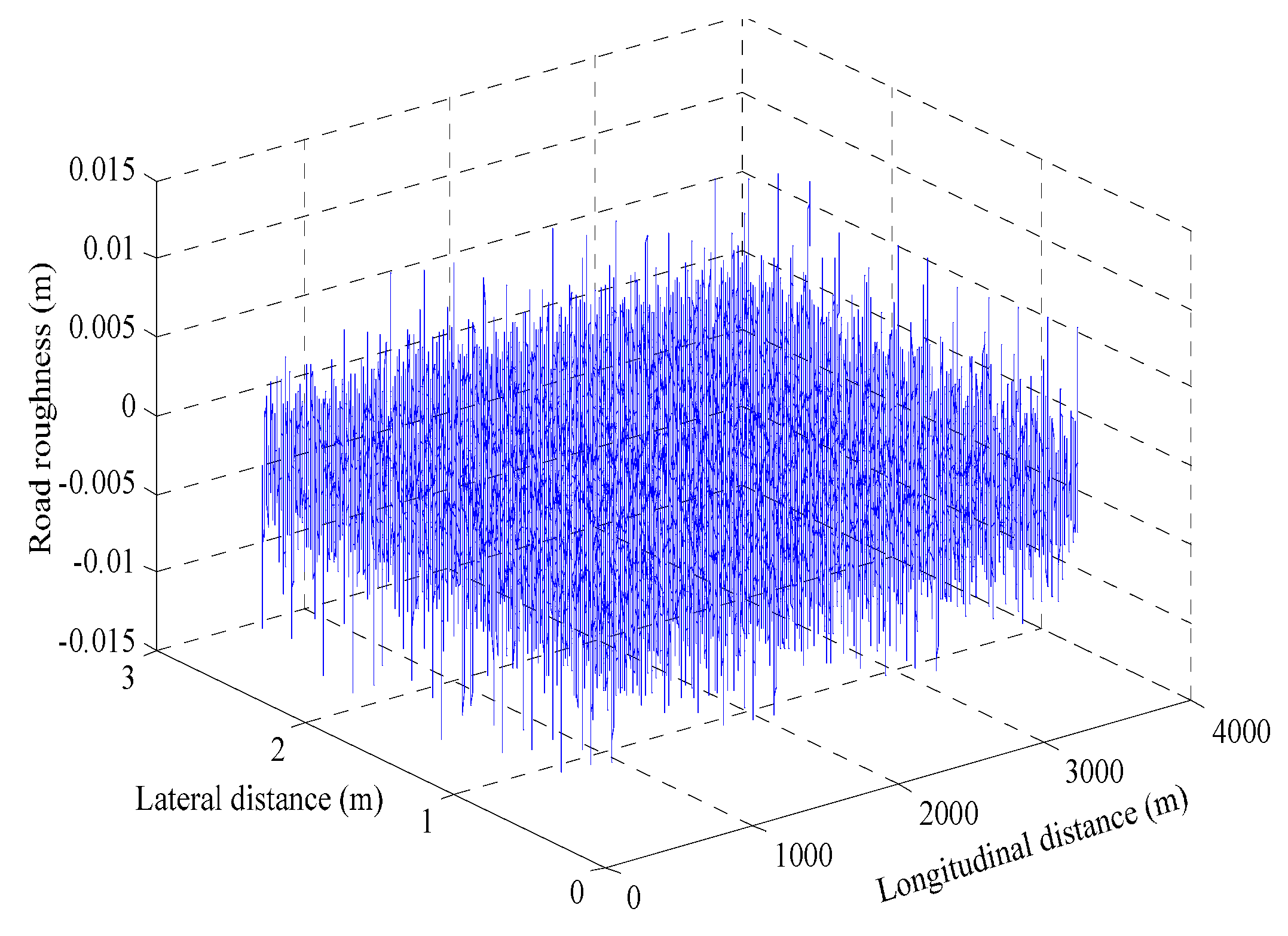
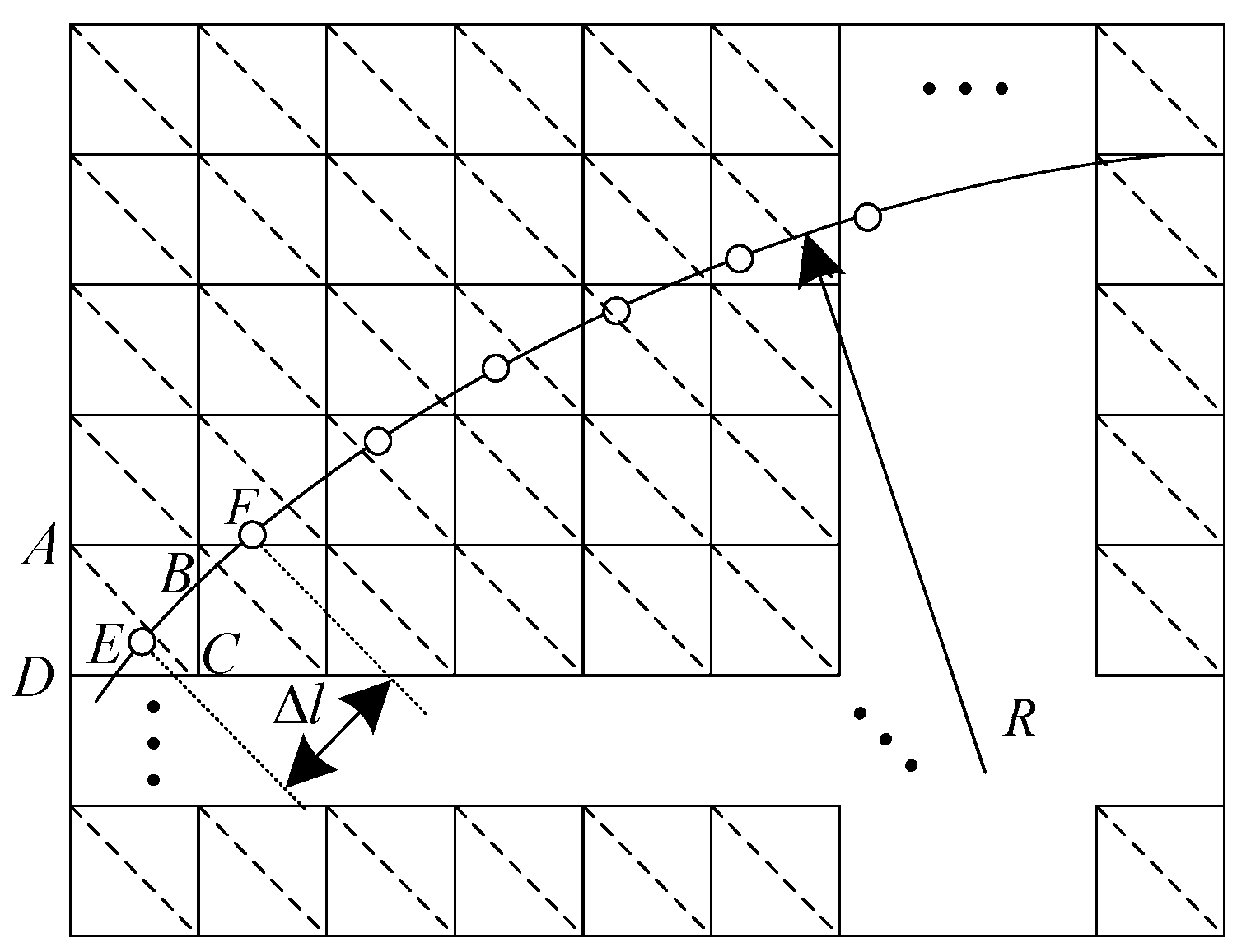
In this paper, a comprehensive analysis considering road excitation and steering wheel input for vehicle roll behavior based on a 6-DOF half-car and a 9-DOF full-car model is proposed. For this analysis, first, a 3-D road profile based on power spectral density (PSD) was developed under straight and steering conditions. Next, 6-DOF and 9-DOF models were constructed under various road conditions. Then, vehicle roll responses using proposed models were obtained with or without the presence of road excitation and various steering wheel input. Finally, CARSIM® was utilized to validate the proposed 6-DOF and 9-DOF models. Results show that vehicle roll performance of 9-DOF model had a significantly higher accuracy than the 6-DOF roll model, especially in presence of road excitation and large steering wheel input.
In order to further illustrate functional relationships between road excitation and vehicle dynamics model, an approach which formulates a relationship between road level and steering wheel input is formulated in this paper. The paper is organized as follows. In
Section 2, a 3-D road profile excitation model is briefly presented. Rollover index is illustrated in
Section 3. In
Section 4, vehicle dynamics of 6-DOF and 9-DOF models are studied.
Section 5 deals with validation of the proposed models using CARSIM
® for various road excitations and different steering wheel input. Finally,
Section 6 concludes the paper.
3. Rollover Index
A common method of defining rollover index (RI) is based on the difference in vertical tire loads between left and right sides of the vehicle [
15].
where
Fzl and
Fzr are vertical tire forces on left and right side tires of the vehicle, respectively. When RI is equal to 1 or −1, right or left wheel lifts off.
Forces on the tire
Fzl and
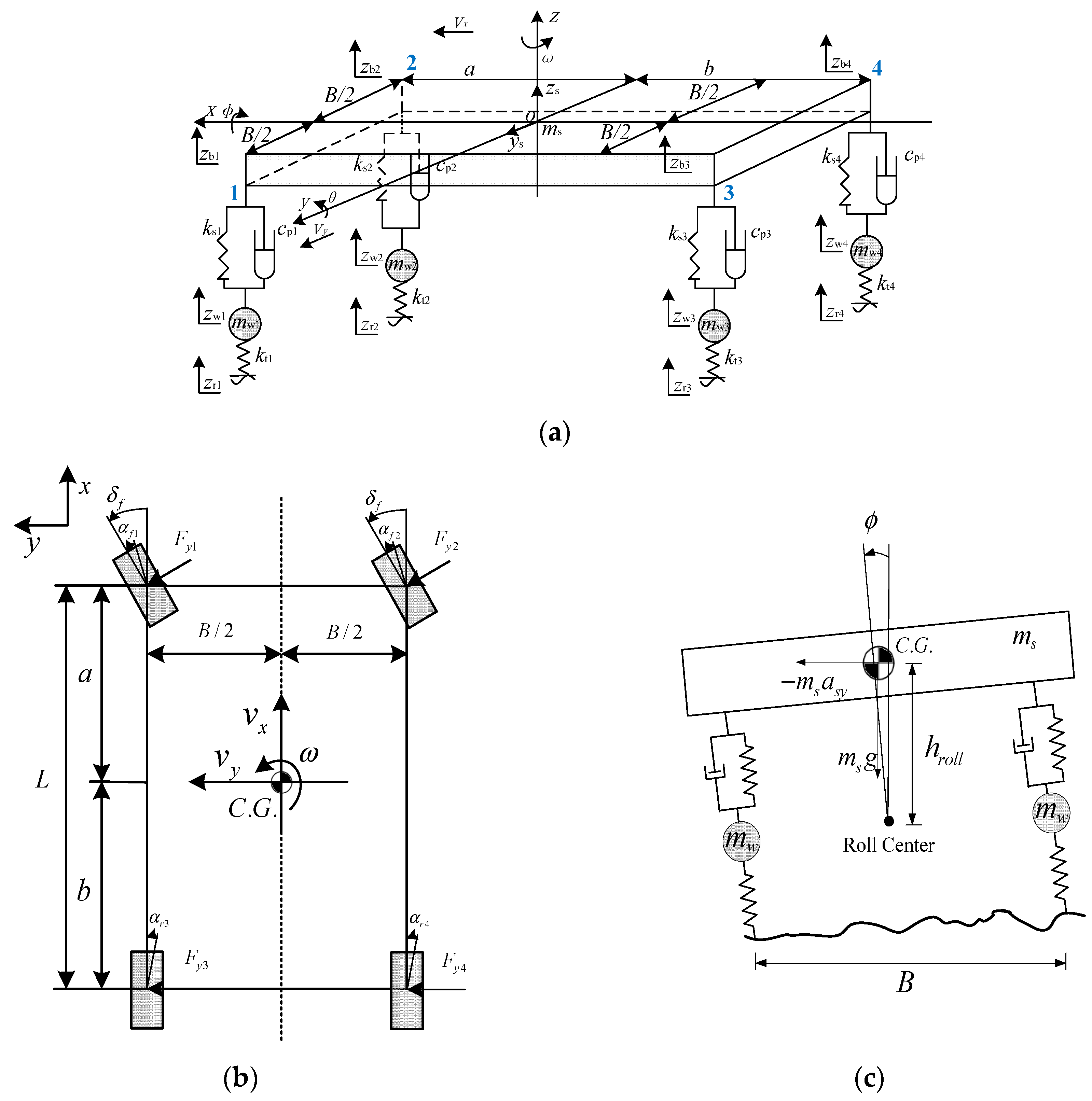
Fzr cannot be directly measured. To obtain RI in this situation, a 4-DOF vehicle model was developed as shown in
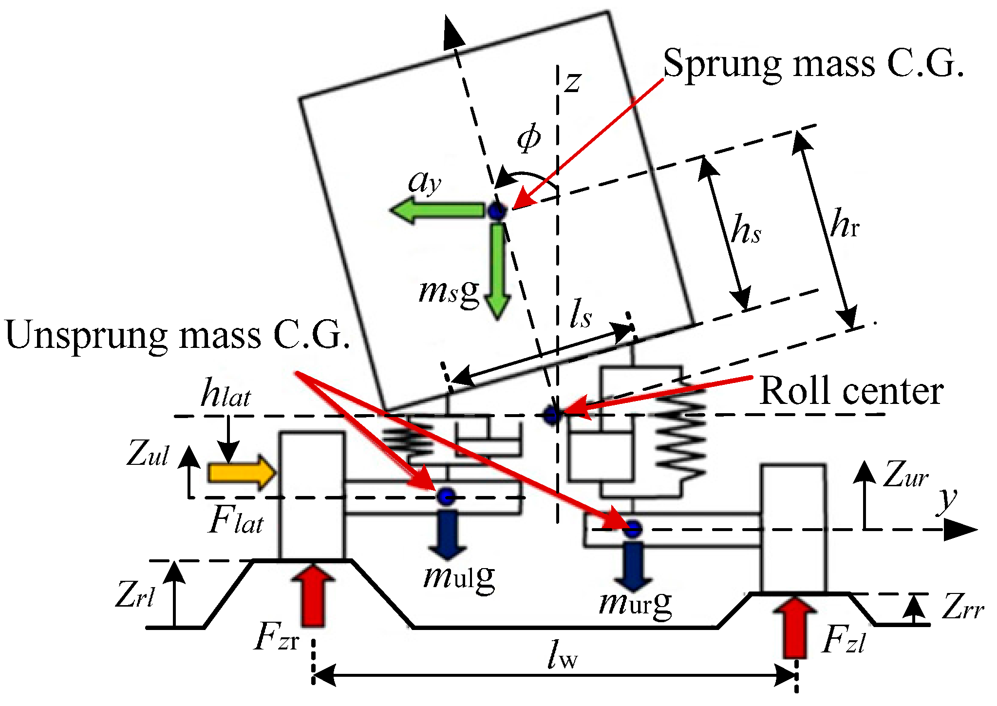
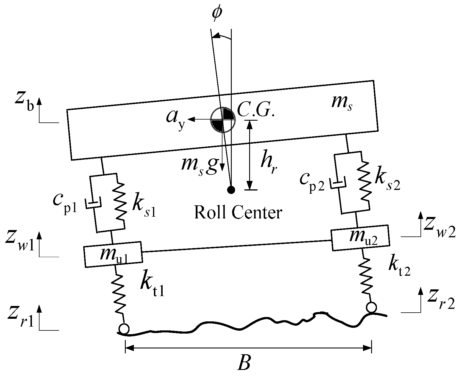
Figure 4, A new RI* can be derived from Equation (15) [
16].
where
hr is distance between C.G. height and roll center;
φ represents roll angle;
ay represents lateral acceleration;
Flat is lateral force;
hlat is distance from input lateral force to roll center;
zrl and
zrr are left and right road excitation, respectively. As shown in
Figure 4,
ls is body distance between left suspension and right suspension, i.e.,
ls is distance of a hinged between suspension and vehicle body;
lw is track width;
ks is suspension stiffness;
zu1 and
zu2 represent left and right unsprung mass positions, respectively;
c is suspension damping;
m is equal to sum of
ms and
mu,
ms and
mu are the sprung mass and unsprung mass of the vehicle, respectively.
5. Simulation and Validation
To validate the two proposed models, an industrial standard vehicle dynamics simulation software, CARSIM
® was used to carry out simulations [
16,
19,
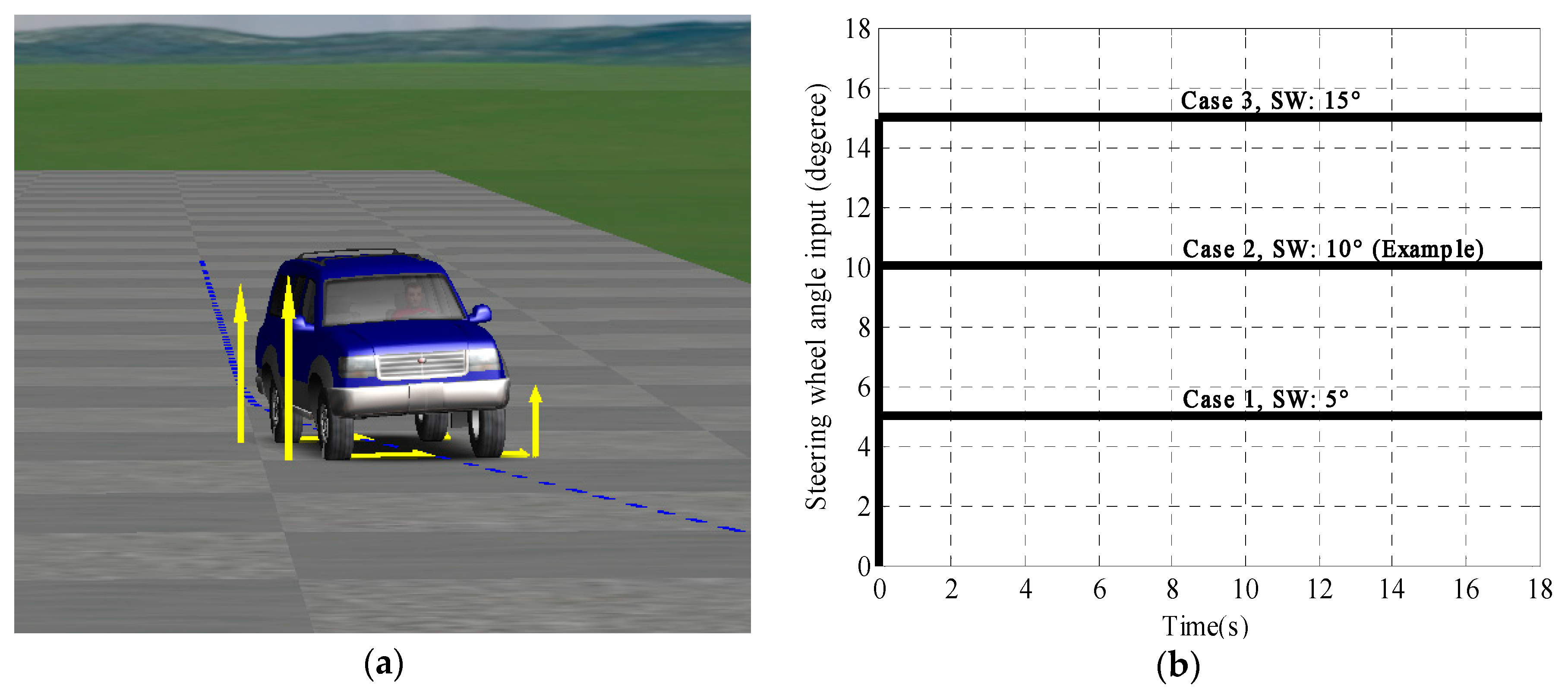
20]. A standard SUV model was chosen from CARSIM
® vehicle models as shown in
Figure 8. Simulation and validation results of vehicle roll behavior were carried out under steering wheel (SW) input 10° condition as an example case to facilitate better analysis of vehicle roll behavior.
Based on the above analysis, half-car and full-car models proposed in
Section 4 were simulated in MATLAB to study performance of vehicle roll behavior with or without road excitation (two representatives). It is assumed that the tire does not loose ground contact. Here, the J-turn maneuver [
15] was utilized to illustrate roll behavior for steering wheel at 10° at a velocity of 80 km/h with presence of road excitation. It was concluded from the results vehicle roll behavior mainly depends on roll angle, roll rate, and yaw rate. It should be noted that roll angle is variable under varying steering wheel input, and roll angle can be seen as a reference validation for vehicle roll behavior.
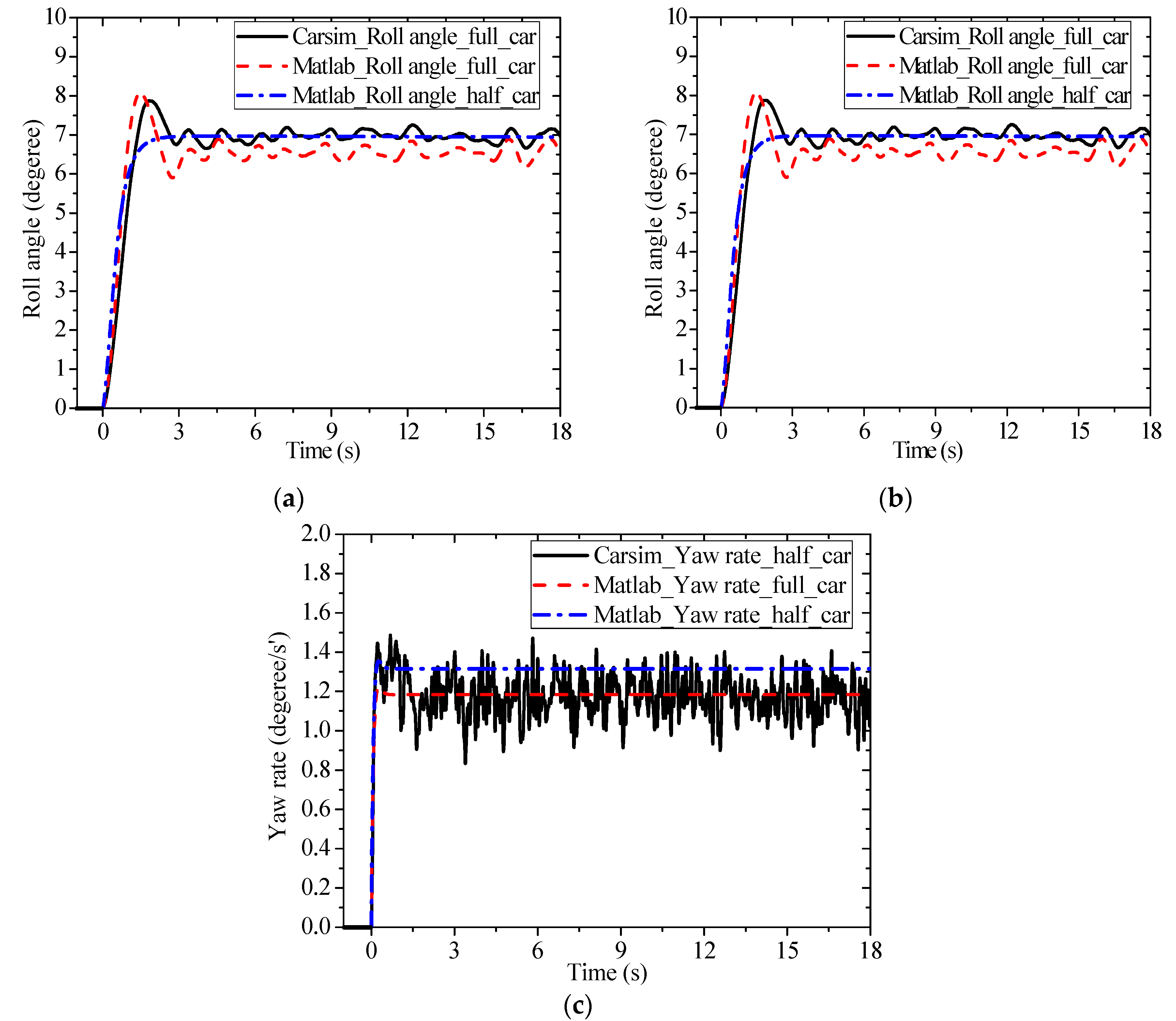
5.1. Roll Behavior without Road Excitation
Here, using vehicle dynamics model from
Section 4, performance of vehicle roll behavior is simulated without presence of road input. Initial conditions used in the simulation are listed in
Table 1 and
Table 2. Corresponding performance of roll behavior result parameters are shown in
Figure 9. It can be seen from
Figure 9 that without road excitation, half-car and full-car model are approximately equivalent. The
E-Class (SUV) level car model in CARSIM
® was used as benchmark results. Calculations carried out in MATLAB were found to be consistent with the CARSIM data. This suggests that vehicle dynamics model presented in
Section 4 can be considered accurate to depict system dynamics under this condition.
5.2. Considering Road Excitation
Case1: Level ISO-A road excitation
Based on the vehicle dynamics model presented in
Section 4, performance of vehicle roll behavior was also computed considering level ISO-
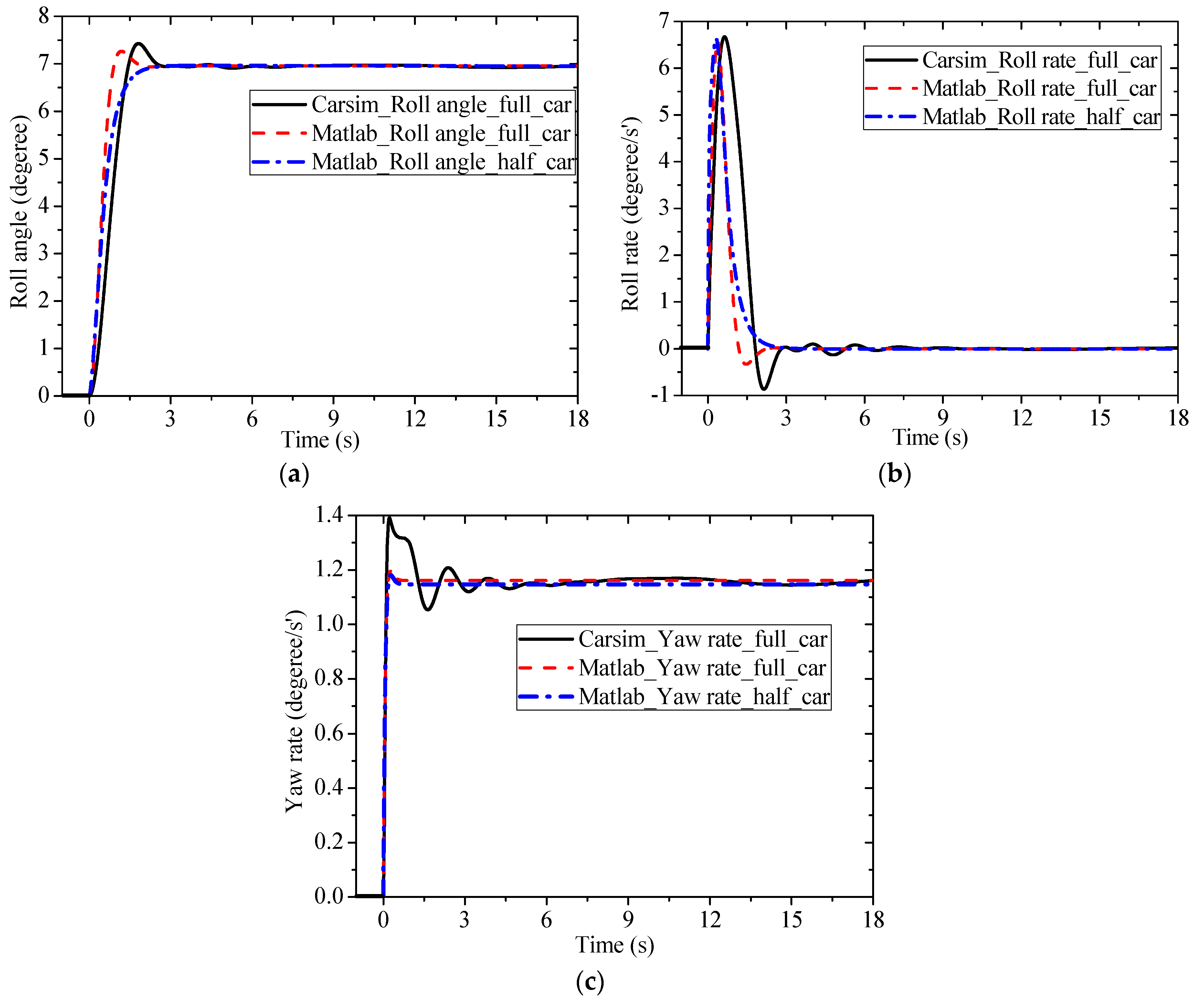
A road excitation. Roll angle, roll rate, and yaw rate for roll behavior are shown in
Figure 10. From the results, it can be seen that with road excitation, vehicle roll responses are different under level ISO-
A road excitation. With
E-Class (SUV) level car model in CARSIM
® as a benchmark, simulation data of 9-DOF full-car model was found to be consistent with CARSIM data, i.e., half-car roll model and full-car roll model are no more equivalent.
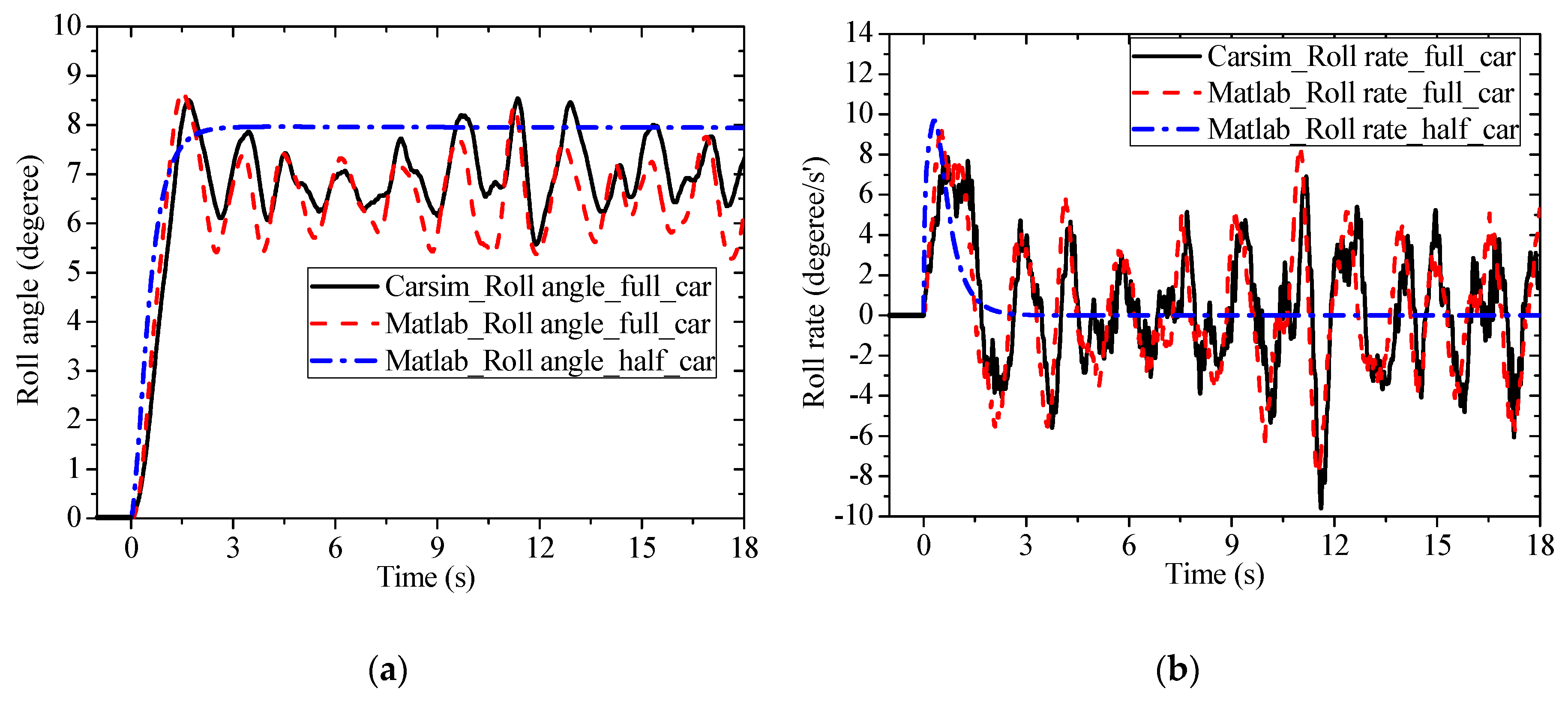
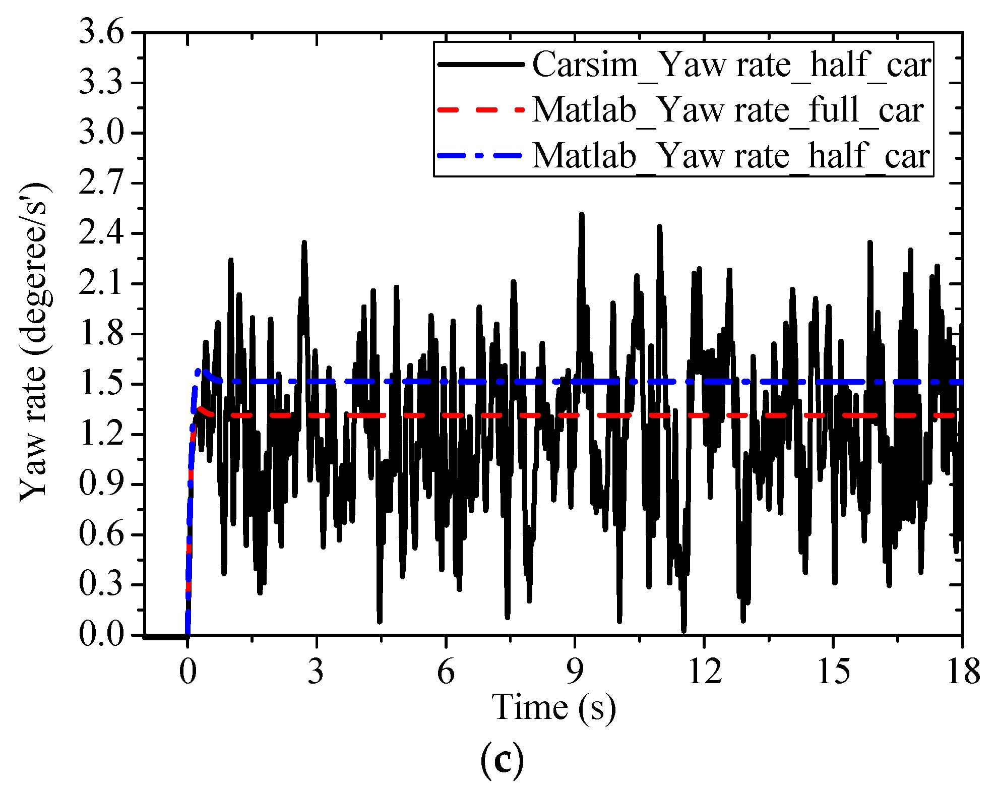
Case 2: Level ISO-C road excitation
For level ISO-
C road excitation case, roll angle, roll rate, and yaw rate for roll behavior are shown in
Figure 11. It can be seen from the results that vehicle response for different dynamics models have significant impact on roll behavior under level ISO-
C road excitation, and influence of road excitation cannot be ignored in this situation [
21,
22,
23,
24,
25,
26,
27].
To further illustrate difference between 6-DOF and 9-DOF models with road excitation and various steering wheel inputs, vehicle responses were statistically analyzed. Previous research divided statistical parameters into dimensional parameters and non-dimensional parameters [
21]. Dimensional parameters such as mean value, variance, maximum, etc., are used to depict steady stochastic processes especially suitable for statistical process description. Non-dimensional parameters, including Kurtosis, Crest factor, Clearance factor, etc., are utilized to describe transient processes, especially suitable for non-statistical process description. Vehicle steering wheel input is a transient response; due to this non-dimensional parameters should be adopted to study vehicle responses. Five widely applied features that suitable for depicting these temporary characteristics as listed in
Table 4 [
22,
23]. Parameter
F1 and
F4 may indicate distribution characteristics. Parameters
F2~
F3,
F5 represent influence of impact or impulse input.
To illustrate error in different dynamics models, with
E-Class (SUV) level car model in CARSIM
® as a benchmark, accuracy of proposed models and comparison results are summarized in
Table 5 and
Table 6.
Table 5 and
Table 6 show that different dynamics models have significant impact on the calculation accuracy, and higher accuracy using 9-DOF model can be obtained when coupling relationships exists between road excitation and vehicle dynamics.
5.3. Disscussion
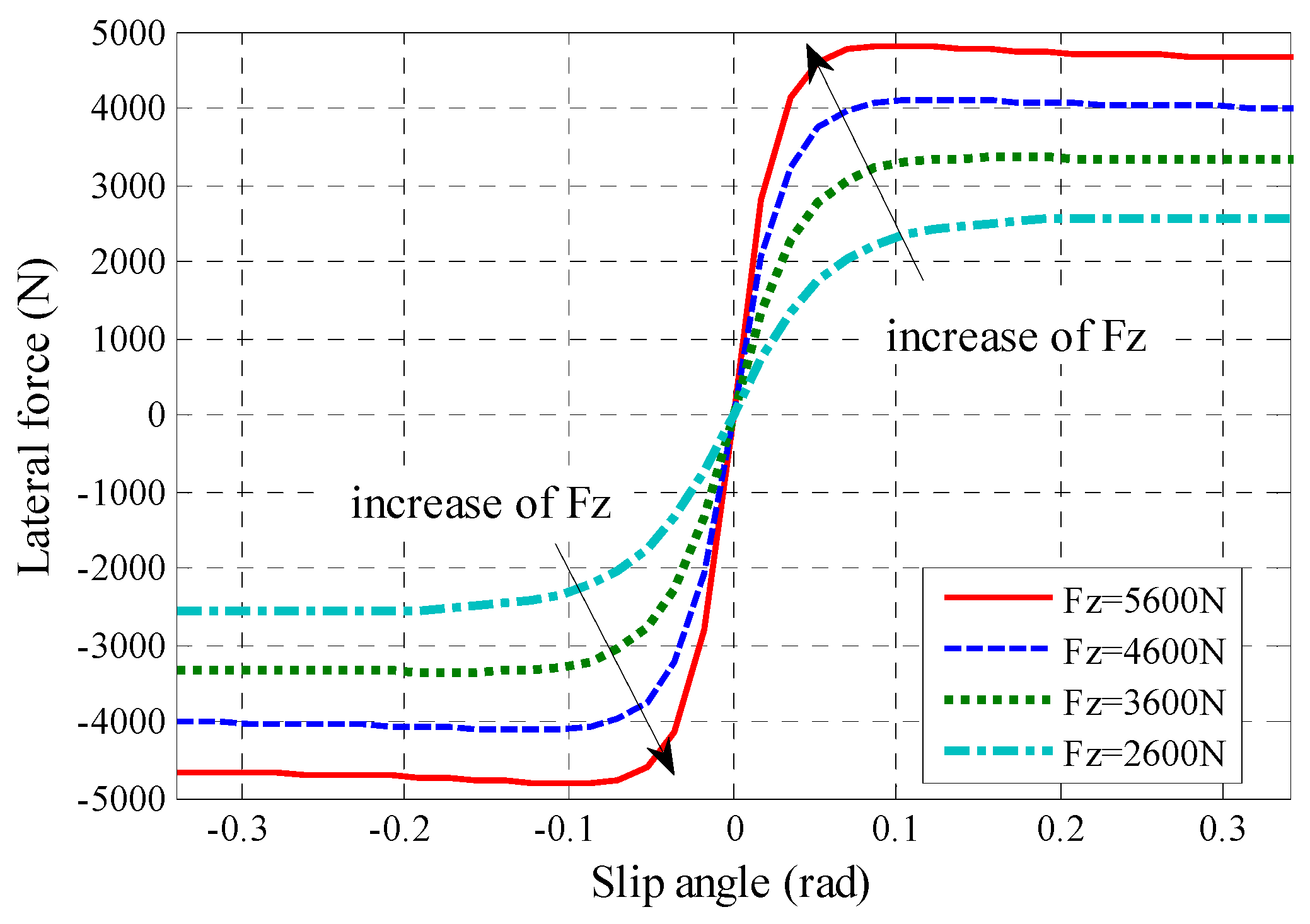
From results in
Figure 6, it can be seen that under identical vertical loads, when slip angle was smaller than 0.08 rad, lateral force on front rear tires increases linearly with increase in slip angle. However, when slip angle was larger than 0.08 rad, rate of lateral force increment gradually slows down, and relationship with slip angle is no longer linear. In addition, for identical slip angles, a larger vertical load was accompanied by a larger lateral force. Thus, for the tire model, lateral force is a function of slip angle and vertical load. Relationships between slip angle and vertical load were nonlinear [
18]. This leads to nonlinear behavior of tire lateral forces under various steering wheel inputs.
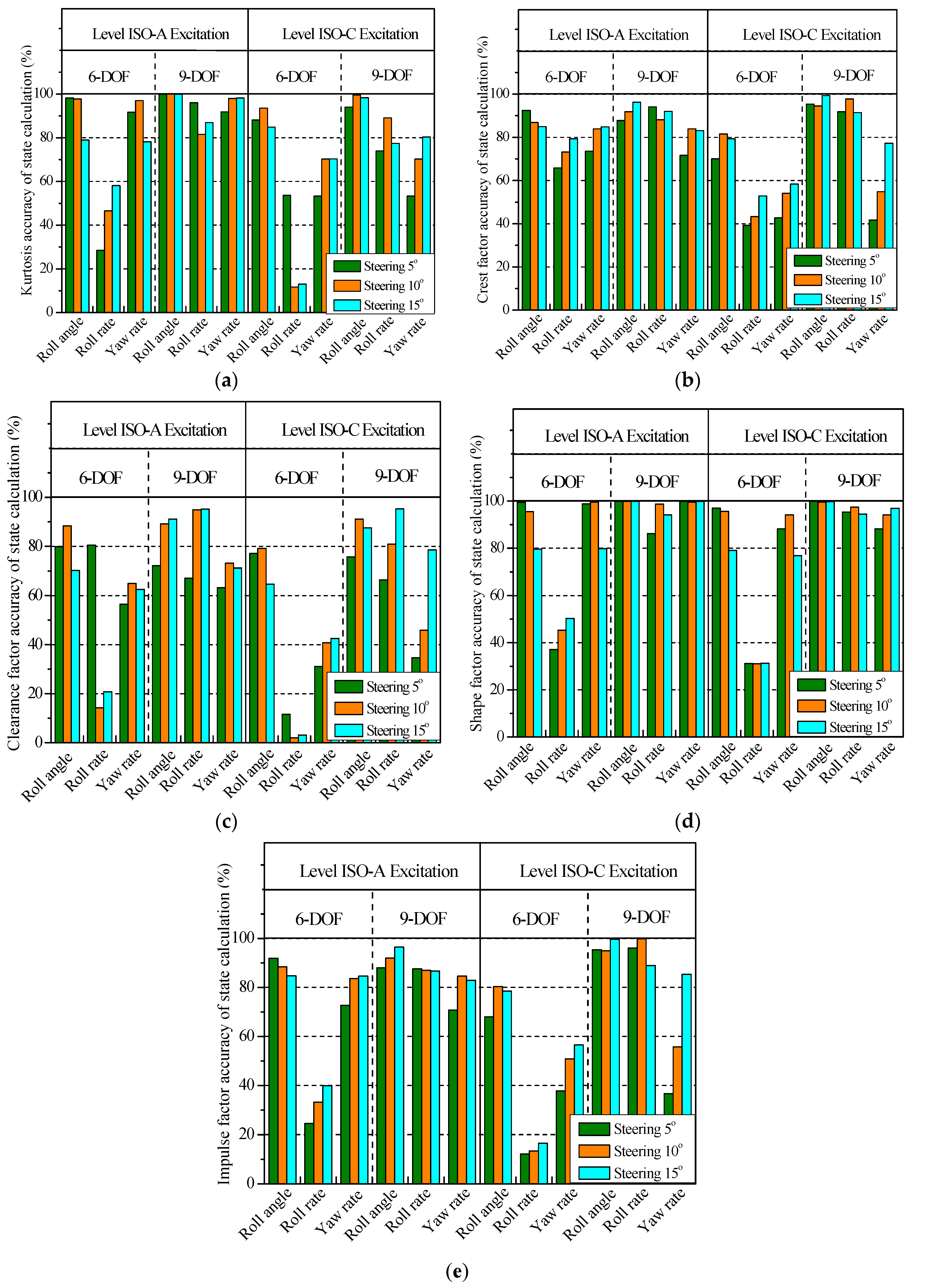
To further illustrate superiority of the proposed model, 5° and 15° steering wheel input situations were also simulated. Similar results were obtained without road excitation, i.e., 6-DOF half-car model and 9-DOF full-car model are approximately equivalent under these conditions. However, 6-DOF model and 9-DOF model have significant differences with road input. Corresponding simulation results for different steering wheel inputs and various road excitations are shown in
Table 7,
Table 8,
Table 9 and
Table 10, which are described as shown in
Figure 12. In
Figure 12a, feature
F1, comparison of 6-DOF and 9-DOF models for road level ISO-
A/
C excitation is shown. It can be seen that accuracy of vehicle responses were higher under road level ISO-
A excitation than road level ISO-
C, i.e., higher road level lead to higher error. Roll angle and roll rate accuracy for vehicle responses of 6-DOF model was a maximum of 60% under road level ISO-
A/
C excitation. Roll angle and roll rate calculation accuracy for vehicle responses of 9-DOF model was 85% under road level ISO-
A/
C excitation. With increase of the steering wheel input, as in the case of
F2, accuracy for 6-DOF model was a maximum of 58% under road level ISO-
A/
C excitation. However, for a 9-DOF model accuracy declined at a slower rate than 6-DOF model as shown in
Figure 12b. From
F3 perspective, an increase in road level resulted in accuracy for vehicle responses of 6-DOF and 9-DOF model to reach a maximum of 90% under road level ISO-
A/
C excitation. However, for a 6-DOF model accuracy declined at a faster rate than 9-DOF model as shown in
Figure 12c. Further, from
F4 and
F5 perspectives,
Figure 12d,e show that accuracy of 9-DOF model vehicle responses are higher under road level ISO-
C excitation and steering wheel input 15° than 6-DOF model vehicle responses under road level ISO-
A excitation and steering wheel input 5°.
Based on the above analysis, simulation results show that accuracy of statistical features calculation for 6-DOF model reached a maximum of 65% for all situations. Lower accuracy of statistical features follows increase in the angle of steering wheel input; accuracy of statistical features calculated for 9-DOF model was higher than 85%.
Comparison of simulation results from MATLAB and CARSIM® allows verification of the proposed 9-DOF full-car model for roll behavior with or without road excitation condition. A 6-DOF half-car model was found to be suitable in conditions without road excitation. Influence of vehicle model on roll behavior should be adopted for the full-car model while analyzing vehicle roll behaviors with large steering wheel input and considering road excitation.
6. Conclusions
In this paper, performance of vehicle roll behavior under various road excitation and steering wheel inputs was studied using 6-DOF half-car and 9-DOF full-car models. With the proposed method, influence of half-car and full-car models on vehicle roll behavior and coupling relationships between vehicle vertical and lateral response was comprehensively studied. The main conclusions are as follows:
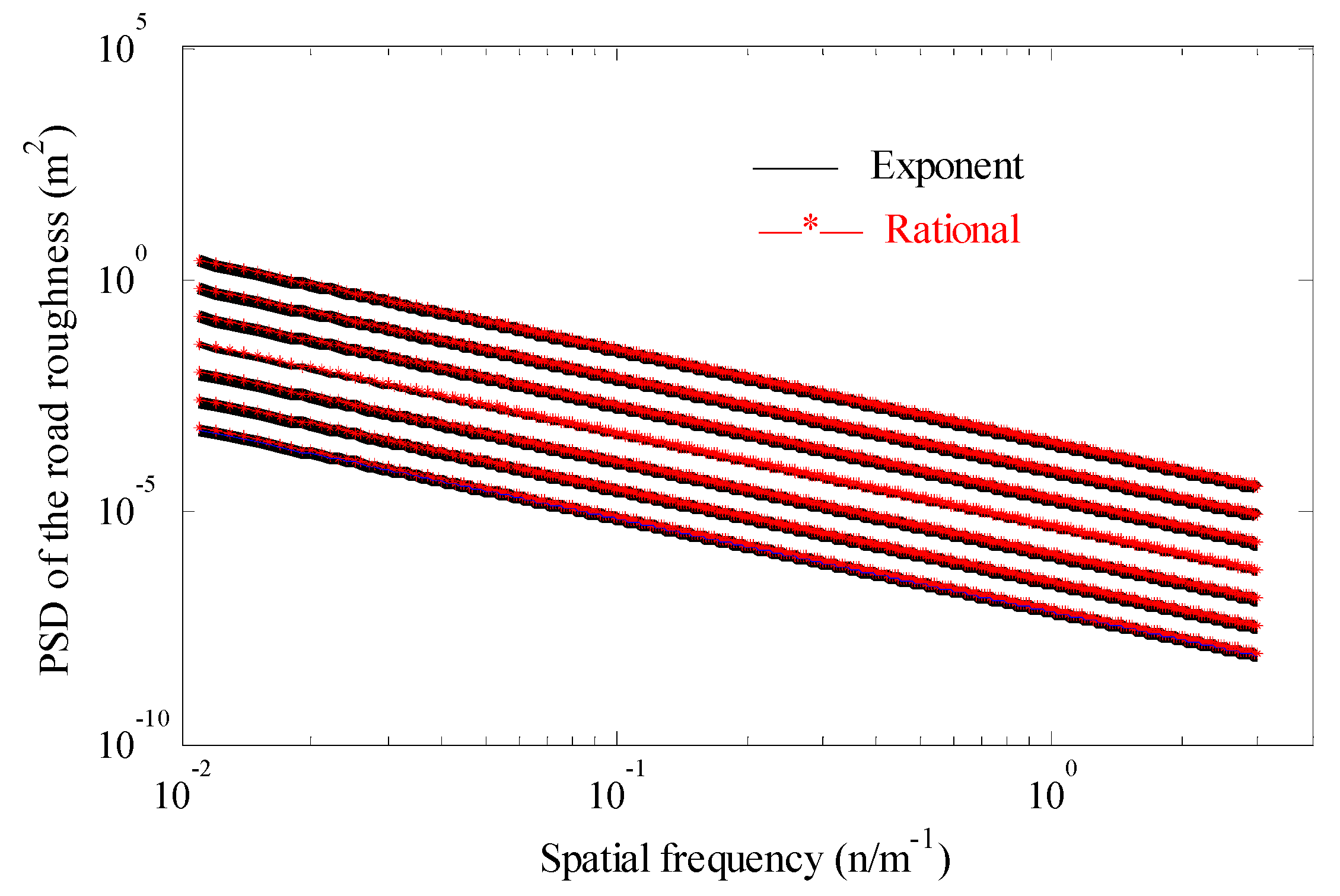
Based on the generating theories, a 3-D road profile model was first developed with road level ISO-A/C as the half-car and full-car dynamics model input. State response of vehicle roll behavior relationships between road excitation and steering wheel input were calculated with half-car and full-car models. From the results, it was concluded that road excitation and steering wheel input have a significant influence on vehicle roll behaviors, i.e., 6-DOF model was suitable for small steering wheel input without road excitation. Average accuracy of this model was determined to be a maximum of 65%. A 9-DOF model was more accurate for large steering input with road excitation with an average accuracy higher than 85%.
Calculated vehicle response of vehicle roll behavior was validated using CARSIM®. Compared to calculation results, CARSIM® simulation results showed that proposed half-car model can provide a satisfying result without road excitation. However, full-car model can provide better description of system dynamics under various road excitation and large steering wheel input conditions to further validate the conclusions.
In the future, the proposed model will be applied to an actual road profile and a practical full-car will be realized using the proposed 9 DOF full-car model. In addition, our research will extend to state estimation and control of a full-car nonlinear suspension system and focus on application of these results for improving vehicle performance, especially on the aspects of ride comfort and road handling.


 ,
, 


