Stereophonic Microphone Array for the Recording of the Direct Sound Field in a Reverberant Environment

Abstract

State-of-the-art stereo recording techniques using two microphones have two main disadvantages: first, a limited reduction of the reverberation in the direct sound component, and second, compression or expansion of the angular position of sound sources. To address these disadvantages, the aim of this study is the development of a true stereo recording microphone array that aims to record the direct and reverberant sound field separately. This array can be used within the recording and playback configuration developed in Grosse and van de Par, 2015. Instead of using only two microphones, the proposed method combines two logarithmically-spaced microphone arrays, whose directivity patterns are optimized with a superdirective beamforming algorithm. The optimization allows us to have a better control of the overall beam pattern and of interchannel level differences. A comparison between the newly-proposed system and existing microphone techniques shows a lower percentage of the recorded reverberance within the sound field.

1. Introduction

Sound reproduction systems play an important role in our everyday life. They allow us to listen to recordings from a different place and a past time. Many different methods for the recording and playback of sound exist, utilizing different combinations of microphone and loudspeaker setups. The most common one is a simple stereo reproduction, but there are more complex reproduction techniques, such as wave field synthesis [1] or ambisonics [2]. Even though the state-of-the-art methods achieve a very good accuracy in reproducing sound fields, they do not consider the interaction between the acoustics of the recording and playback environment. In particular, extra reverberation is created by the playback environment, and in addition, there is no control over the spatial distribution of the reverberant sound field, which may influence the apparent source width and perceived listener envelopment. For this reason, ongoing investigations aim to improve the performance of these methods.

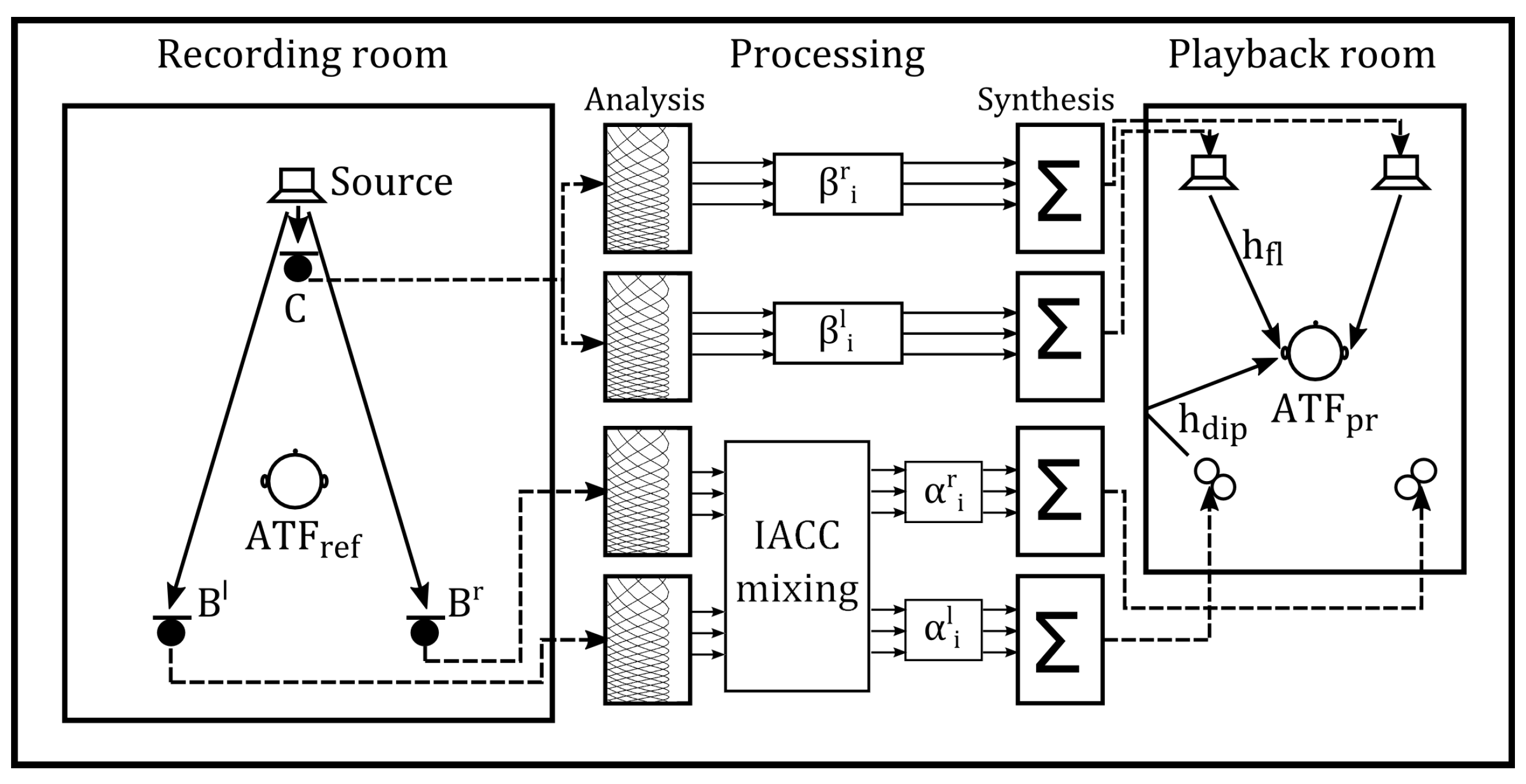
In particular, Grosse and van de Par proposed a new way of recording and playing back sound fields [3]. The main idea behind their research was to record the direct and reverberant sound field separately in order to be able to render it in a playback room while optimizing certain perceptually-motivated criteria for the authentic audio reproduction. These criteria aim for recreating the reverberant sound field in the playback environment as faithfully as possible by optimizing the amount and spectral shape of the reverberation, as well as the interaural cross-correlation created by the reproduced reverberant sound field, such as it is created in the reproduction room, including its added reverberant effect. In their paper, Grosse and van de Par assumed that optimizing these perceptual criteria is sufficient for an authentic reproduction of the sound field present in the recording room, which is created by a single source. This claim was supported by subjective evaluations. The playback and recording configuration can be seen in Figure 1. In addition to the two basic stereo loudspeakers, the proposed approach used two dipole loudspeakers to excite and equalize the reverberant sound field. For the optimized rendering, the system relies on the presence of a relatively dry direct signal to be rendered on the frontal loudspeakers and a reverberant signal to be optimized and rendered on the dipole loudspeakers. To record the direct sound, a microphone $\left(C\right)$ was positioned close to the sound source. This also avoided early reflections, which could cause a change in coloration [4,5]. For recording the reverberant sound field, two microphones $(B^l,B^r)$ were placed at two distant positions in the diffuse field.

Since the method of Grosse and van de Par [3] until now is limited to a single source and only records the direct sound field with one microphone, an extension is needed to also represent the spatial distribution of sources within the direct sound field signals as perceived at the listener position. Although this could in principle be achieved by using multiple close microphones and an appropriate mixing scheme, in this contribution, we want to provide a method with only a single `true-stereo’ microphone setup that is placed at the intended listener position within the recording room. Particular attention has to be paid to reduce the reverberant sound field in the direct sound field signals to be able to separately optimize the rendering of the direct and reverberant sound fields according to perceptual criteria within the playback room [3].

Although the specific design criteria for the proposed microphone array are envisioned to be used in the audio reproduction system of Grosse and van de Par [3], it can also be considered to use the proposed microphone array to record a relatively dry spatial image of the sound sources on stage to be combined with a reverberant track that can be mixed at a level that the recording engineer deems suitable. In this case, however, it will not necessarily fulfill the optimization criteria as formulated in Grosse and van de Par [3] that create a faithful audio reproduction.

The state-of-the-art true stereo systems combine two microphones with a characteristic directivity pattern, placed at different distances and under different angles relative to one another. Depending on these parameters, a deviating spatial rendering of the distributed sources can be observed [6]. Despite this, for use in the method proposed by Grosse and van de Par [3], these systems have some disadvantages that make them unsuitable to be implemented in this specific sound reproduction system because there is a high percentage of recorded reverberant sound, which should be avoided in the system of [3].

We overcome these disadvantages with the development of a new method of a true stereo microphone array, using a superdirective beamforming algorithm that is applied on two logarithmically-spaced microphone arrays. Correct, frequency-dependent interchannel level differences are captured by optimizing the shape of the two main lobes of the arrays. Together, they create the proper interchannel level difference required for an accurate spatial reproduction of the sound field while ensuring that no interchannel phase differences occur that can result in unintended changes in the perceived location of sound sources. Additionally, an optimal side lobe suppression is applied to reduce the influence of the reverberant sound field on the recording of the direct sound. This proposed stereo microphone array is compared to the state-of-the-art stereo microphone configurations mentioned earlier that shows a clearly reduced level of the reverberant sound field.

2. Methods

The following section is divided into five parts. The first Section 2.1 gives a brief introduction to the most relevant theory on beamforming needed for our proposed method. Section 2.2 focuses on the issue of the robustness of beamforming algorithms. The desired directivity pattern is specified in Section 2.3, which is based on a stereo intensity-panning rule related to the auditory processing of the interaural level differences. Section 2.4 introduces an optimal array design to suppress side lobes and, in this way, reduce the influence of the reverberant sound field on the recording of the direct sound. Further, a specific filter design is proposed in Section 2.5, which will be used and evaluated throughout this study. The design is based on a superdirective beamforming algorithm and describes how the directivity pattern that is specified in Section 2.3 can be used for the optimization.

2.1. Beamforming

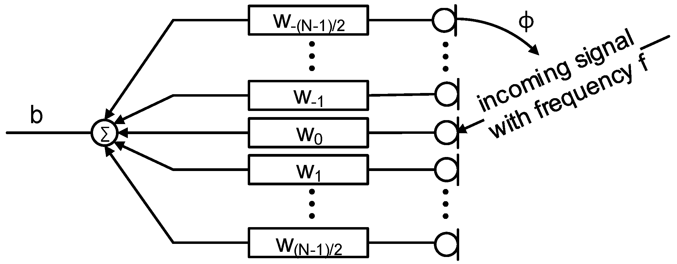
Beamforming describes the process of forming the directivity pattern of several microphones, which are arranged into an array, with signal processing techniques to obtain a specific, frequency-dependent directivity pattern. The directivity pattern $b(f,\varphi )$ of a linear discrete microphone array, consisting of N microphones, is calculated as follows [7]:

$$b(f,\varphi )=\sum _{n=-\frac{N-1}{2}}^{\frac{N-1}{2}}{w}_n\left(f\right)G_n(f,\varphi )$$

(1)

where $\varphi$ denotes the angle ranging from $-\mathsf{\pi }$ to $\mathsf{\pi }$, f the frequency, $w_n\left(f\right)$ the frequency-dependent complex weighting filtering applied to microphone n and $G_n(f,\varphi )$ the steering vector denoting the direction and frequency-dependent transfer function from the sound source to microphone n. Such a microphone array is illustrated in Figure 2.

Assuming a far field condition with the microphones that have an omnidirectional directivity pattern, the transfer function states:

$$G_n(f,\varphi )=e^{-i\frac{2\mathsf{\pi }f}{c}{x}_{n}cos\left(\varphi \right)}$$

(2)

where c is the speed of sound and $x_n$ represents the distance of the n-th microphone to the center of the array [7].

The influence on the directivity patterns of the microphones in the array can be taken into account by changing the transfer function $G_n$. The filter optimization used to match the directivity pattern of the array with a desired one is called beamforming. The look direction of the microphone array is defined as the angle of the main lobe of the desired directivity pattern, which is also called the steering angle.

There are several beamforming algorithms based on an analytic solution for the optimal filter $w_n\left(f\right)$ and some others on a numerical approximation. Analytic solutions allow us to set N constraints on the directivity pattern for a finite number of frequencies, as for example described in [8]. Since we have a higher number of constraints in our problem, we will use numerical methods that allow accommodating a higher number of constraints to control the directivity pattern.

Equation (1) will be solved numerically, and for this purpose, the frequency range is discretized into P frequencies $f_p,p=0,\cdots ,P-1$ and the angular range into M angles ${\varphi }_m,m=0,\cdots ,M-1$:

$$b(f_p,{\varphi }_m)=\sum _{n=-\frac{N-1}{2}}^{\frac{N-1}{2}}{w}_n\left(f_p\right)G_n(f_p,{\varphi }_m)$$

(3)

Equation (3) is reformulated in matrix notation as:

$${\mathbf{b}}_m\left(f_p\right)={\mathbf{G}}_{mn}\left(f_p\right){\mathbf{w}}_n\left(f_p\right)$$

(4)

where the directivity pattern is an $M\times 1$ vector ${\mathbf{b}}_m^T\left(f_p\right)=[b(f_p,{\varphi }_0),b(f_p,{\varphi }_1),\cdots ,b(f_p,{\varphi }_{M-1}]$, the transfer function an $M\times N$ matrix ${\left[\mathbf{G}\left(f_p\right)\right]}_{mn}=e^{-i\frac{2\mathsf{\pi }{f}_p}{c}{x}_{n}cos\left({\varphi }_m\right)}$ and the filter a $N\times 1$ vector ${\mathbf{w}}_n\left(f_p\right)={[w_{-\frac{N-1}{2}}\left(f_p\right),w_{-\frac{N-3}{2}}\left(f_p\right),\cdots ,w_{\frac{N-1}{2}}\left(f_p\right)]}^T$ [7]. All bold variables are either vectors or matrices in the remainder of this manuscript.

2.2. Robustness and White Noise Gain

One of the problems that beamforming algorithms often have is their lack of robustness. This property is related to a resistance to the presence of spatially white noise and can be impaired by deviations from the specified microphone characteristics and microphone position errors. These imperfections affect the beamformer in a manner similar to a recorded spatially white noise that is amplified. Hence, the White Noise Gain (WNG) is a measure commonly used for quantifying the robustness of a beamformer design. The WNG shows the ability of a beamformer to suppress spatial white noise, because it expresses the gain of the beamformer in the desired look direction relative to the amplification of spatially white noise.

The WNG $A\left(f_p\right)$ is defined as follows:

$$A\left(f_p\right)=\frac{{\left|b_{steer}\left(f_p\right)\right|}^2}{{\mathbf{w}}_n^H\left(f_p\right){\mathbf{w}}_n\left(f_p\right)}$$

(5)

where $b_{steer}\left(f_p\right)$ denotes the value of the directivity pattern in steer direction [7]. A high value of the WNG $A\left(f_p\right)>1$ corresponds to a robust beamforming design, whereas a small value $A\left(f_p\right)<1$ effectively corresponds to an amplification of spatial white noise [7]. The maximum possible value of the WNG is equal to the number of microphones used:

$$max\left(A\left(f_p\right)\right)=N$$

(6)

which corresponds to a uniform filter [7]:

$$|w_n\left(f_p\right)|=\frac{1}{N}$$

(7)

2.3. Desired Directivity Pattern

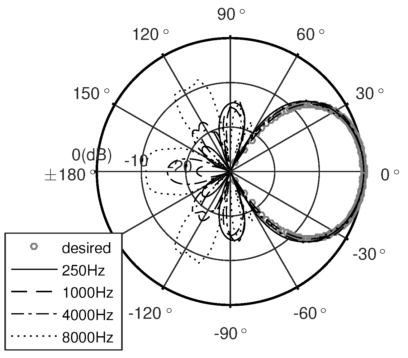
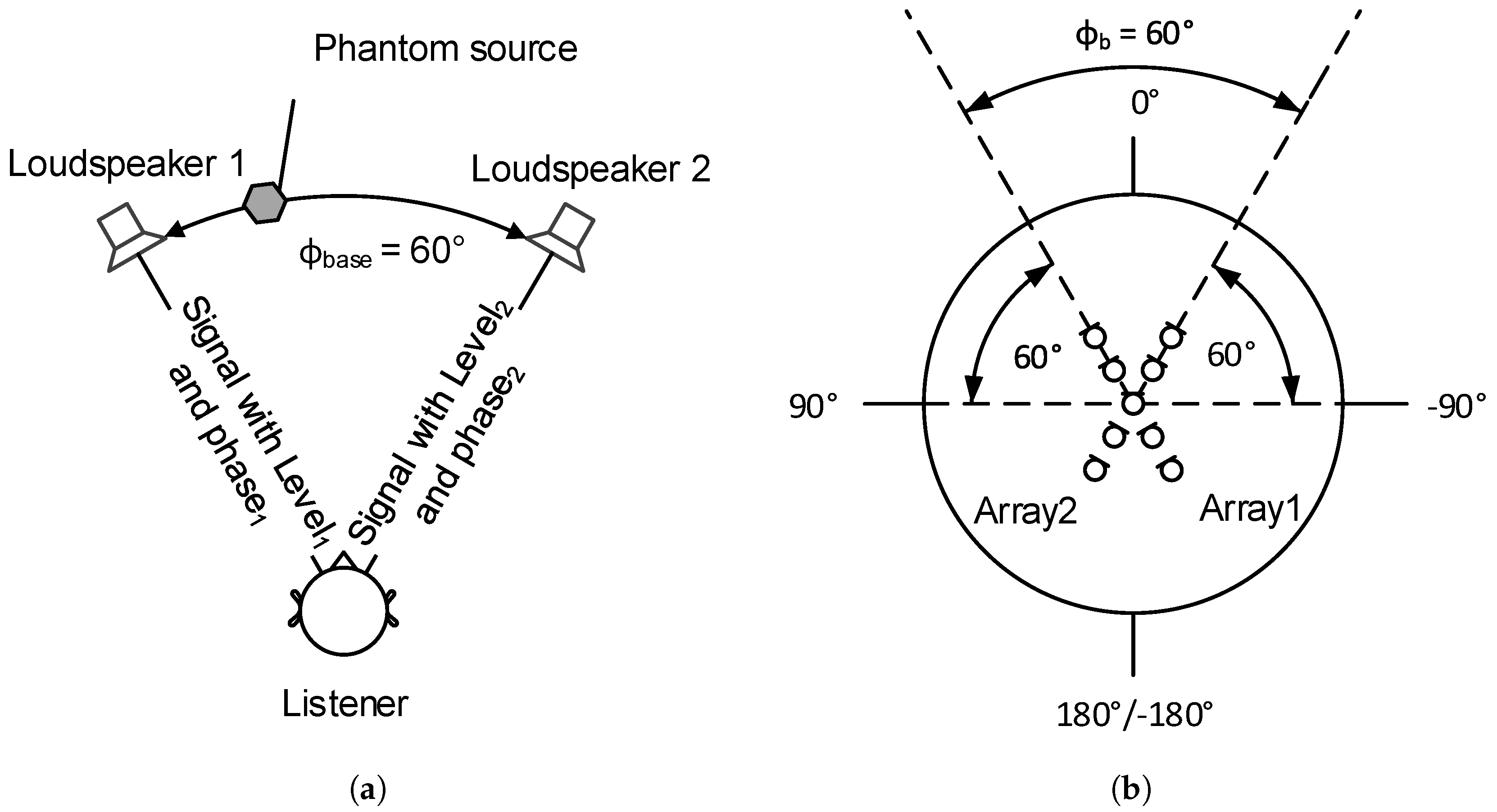
The playback of the recorded signals should be in a stereophonic configuration, as mentioned in Section 1 and illustrated in Figure 3a.

The playback approach proposed by Grosse and van de Par [3] uses two loudspeakers for the direct sound reproduction with a typical base angle of ${\varphi }_{base}={60}^{\circ }$ relative to the listener’s position [9]. There are several approaches to shift a phantom source from one loudspeaker to the other, utilizing phase differences $\Delta phase=phas{e}_1-phas{e}_2$ and/or level differences (amplitude panning) $\Delta Level=Leve{l}_1-Leve{l}_2$ applied on the two loudspeaker signals.

Based on this playback configuration, the recording configuration presented in this paper consists of two crossed end-fire microphone arrays with a ${60}^{\circ }$ opening angle, sharing one center microphone and using omnidirectional microphones, illustrated in Figure 3b. The microphone positions in this figure can only be considered as a sketch, the absolute positions can be found in Section 3. The phantom-source shifting approaches of the playback configuration can be used to formulate either the correct phase and/or level differences between the two arrays. In this way, the perceived location of the sound source in the playback situation is identical to the one of the recording provided that the distribution of recorded sound sources does not span more than ${60}^{\circ }$ of angle. Although not evaluated here, in principle, a different opening angle could be used for the microphone arrays, thus effectively compressing or expanding the reproduced sound stage. We restrict our proposed method to have only level differences, and for this reason, the desired directivity pattern $\widehat{b}$ is purely real valued. With this desired directivity pattern, the phase of the directivity pattern is mainly controlled by the array design, which will be explained in Section 2.4.

In this paper, the phantom source shifting approach of amplitude panning is used for formulating the desired directivity pattern of Array 1 ${\widehat{b}}_{array1}$ and Array 2 ${\widehat{b}}_{array2}$ [9]:

$$\begin{array}{c}{\widehat{b}}_{array1}\left({\varphi }_{\delta }\right)=\sqrt{{\left(1+{\left(\frac{tan\left({\varphi }_{\delta }\right)-tan({\varphi }_b/2)}{tan\left({\varphi }_{\delta }\right)+tan({\varphi }_b/2)}\right)}^2\right)}^{-1}}\hfill \\ {\widehat{b}}_{array2}\left({\varphi }_{\delta }\right)=\sqrt{{\left(1+{\left(\frac{tan\left({\varphi }_{\delta }\right)+tan({\varphi }_b/2)}{tan\left({\varphi }_{\delta }\right)-tan({\varphi }_b/2)}\right)}^2\right)}^{-1}}\hfill \\ \hfill \end{array}$$

(8)

The angle area ${\varphi }_{\delta }$ between both arrays is defined by:

$${\varphi }_{\delta }=\left\{{\varphi }_m|-{\varphi }_b/2\le {\varphi }_m\le {\varphi }_b/2\right\}$$

(9)

with the constant ${\varphi }_b={\varphi }_{base}={60}^{\circ }$. The derivation of the desired directivity patterns according to [9] gives two possible recording room assumptions: an anechoic chamber or a real room. The latter one is chosen for Equation (8) since the microphone array configuration will be used in real rooms, such as concert halls.

The desired directivity pattern of the one array is the mirror-flipped version of the other array. This symmetry of the recording configuration makes it possible to formulate one desired directivity pattern, which is the same for both arrays. The following parts of the desired directivity pattern, the first ${\widehat{b}}_{beam}$ valid for the beam area and the second ${\widehat{b}}_{steer}$ valid for the steering angle, consider a microphone array aligned on the $0^{\circ }$ axis corresponding to the steering angle ${\varphi }_{steer}=0^{\circ }$:

$${\widehat{b}}_{beam}=\left\{\begin{array}{cc}\sqrt{{\left(1+{\left(\frac{tan(\varphi +{\varphi }_b/2)-tan({\varphi }_b/2)}{tan(\varphi +{\varphi }_b/2)+tan({\varphi }_b/2)}\right)}^2\right)}^{-1}}\hfill & \mathrm{for}-{\varphi }_b\le \varphi <0^{\circ }\hfill \\ \sqrt{{\left(1+{\left(\frac{tan(\varphi -{\varphi }_b/2)+tan({\varphi }_b/2)}{tan(\varphi -{\varphi }_b/2)-tan({\varphi }_b/2)}\right)}^2\right)}^{-1}}\hfill & \mathrm{for}{0}^{\circ }<\varphi \le {\varphi }_b\hfill \end{array}\right.$$

(10)

$${\widehat{b}}_{steer}({\varphi }_{steer}=0^{\circ })=1$$

(11)

In the following subsections, an optimal array design in terms of optimal microphone positions and an optimal filter design is proposed to achieve the desired directivity pattern.

2.4. Array Design

The positions of the microphones have an influence both on the filter ${\mathbf{w}}_n\left(f_p\right)$ and the transfer function ${\mathbf{G}}_{mn}\left(f_p\right)$, and thus, on the directivity pattern itself. The optimal microphone positions selected for this paper maximize the spatial aliasing frequency and, at the same time, minimize the frequency from which beamforming is effectively possible. The spatial aliasing frequency describes the lowest frequency $f_{al}$ for which aliasing effects occur, which is caused by a spatial undersampling of the array for sound waves at high frequencies. The aliasing leads to side lobes with the same amplitude as the main lobe. The spatial aliasing frequency of an array with linear microphone spacing is usually given in the literature as:

$$f_{al}=\frac{c}{2\mathrm{▵}x}$$

(12)

with $\mathrm{▵}x$ as the space between the microphones [10].

A small microphone spacing sets an upper limit to the spatial aliasing frequency. In contrast, a large microphone spacing sets a lower limit to the frequency from which beamforming is effectively possible. In order to have good directional properties of the microphone array across a wide frequency range, an irregularly-spaced microphone array is used in which both kinds of spacing can occur. A linear-shaped, logarithmically-spaced, to the reference microphone ($n=0$), symmetrical array is used in this paper. Consequential, the number of the used microphones N has to be uneven $(N\in {\mathbb{N}}_U)$. The symmetry around one central microphone ensures a purely real directivity. The microphone positions are calculated as follows [11].

$$\begin{array}{c}\hfill (x_{n+1}-x_n)=(x_n-x_{n-1})\xi \mathrm{if}n>0\\ \hfill (x_{n-1}-x_n)=(x_n-x_{n+1})\xi \mathrm{if}n<0\end{array}$$

(13)

with:

$$\begin{array}{cc}\hfill x_0& =0\hfill \\ \hfill \xi & ={\left(l_{spread}\right)}^{\frac{2}{N-3}}\hfill \\ \hfill (x_1-x_0)& =(x_0-x_{-1})=\frac{Length}{2{\sum }_{n=1}^{\frac{N-1}{2}}{\xi }^{n-1}}\hfill \end{array}$$

where $Length$ is the total length of the array. The array parameter $l_{spread}\in {\mathbb{R}}^{>0}$ is a free variable describing the ratio between the spacing of the microphones at the extremities of the array and the spacing of the microphones at the center of the array. Linear microphone spacings are archived with $l_{spread}=1$. If $l_{spread}<1$, the spacing of the microphones at the extremities of the array is smaller than the one at the center of the array. In the case of $l_{spread}>1$, it is the opposite.

2.5. Filter Design

In this section, an optimal filter design is proposed to fit the directivity pattern of the array, whose design was specified in Section 2.4, to the desired directivity pattern specified in Section 2.3. The following filter design is based on numerical convex optimization and has the advantage that only one global minimum exists. In general, this end-fire design can also be used with different desired directivity patterns and array designs. In Section 3, we indicate the ideal values of the constants for the desired directivity pattern and array design proposed in this study.

The aim of this algorithm is to minimize the quadratic error ${\mathbf{error}}_m$ between the directivity pattern obtained by a microphone array ${\mathbf{b}}_m\left(f_p\right)$ and a desired frequency independent directivity pattern ${\widehat{\mathbf{b}}}_m$ [7]:

$$\begin{array}{c}{\mathbf{error}}_m={\mathbf{G}}_{mn}\left(f_p\right){\mathbf{w}}_n\left(f_p\right)-{\widehat{\mathbf{b}}}_m={\mathbf{b}}_m\left(f_p\right)-{\widehat{\mathbf{b}}}_m\hfill \\ \underset{{\mathbf{w}}_n\left(f_p\right)}{min}{\parallel {\mathbf{error}}_m\parallel }_2^2\hfill \end{array}$$

(14)

This minimization task will be subjected to additional constraints, and therefore, the beamformer will be termed the Constrained Least-Squares Beamformer (CLSB).

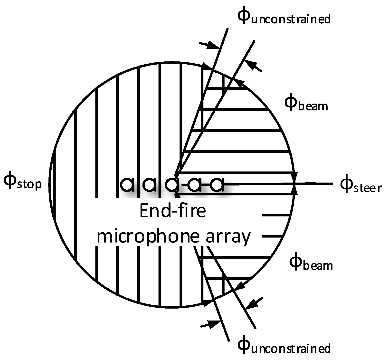
In the following subsections, the main minimization task and the used constraints will be explained paying particularly attention to the WNG and different spatial areas. These areas are shown in Figure 4.

Additionally, this optimization process is placed within an optimization loop in order to optimize several important constants. This optimization procedure will be explained in the last subsection of this section.

2.5.1. White Noise Gain

Such a convex optimization procedure allows including a frequency-dependent lower bound $\gamma \left(f_p\right)$ for the WNG when optimizing the filters $w_n\left(f_p\right)$ [7]:

$$\begin{array}{cc}\hfill A\left(f_p\right)& =\frac{|b_{steer}\left(f_p\right){|}^2}{{\mathbf{w}}_n^H\left(f_p\right){\mathbf{w}}_n\left(f_p\right)}\ge \gamma \left(f_p\right)\hfill \\ \hfill & \mathrm{with}\gamma \left(f_p\right)\in {\mathbb{R}}^{\ge 0}\hfill \end{array}$$

(15)

This constraint has a direct influence on the robustness and on how well the desired directivity pattern can be achieved. A high value for the lower bound reduces the accuracy of forming the directivity pattern because the filter is too restricted by this constraint, whereas a low value leads to a not robust filter. In Section 3, an optimal value for this lower bound will be discussed.

2.5.2. Steering Angle

In the direction of the steering angle ${\varphi }_{steer}$, representing the direction of the main lobe of the microphone array, the directivity pattern obtained by the array is constrained to the value of the desired directivity pattern [7]:

$${\mathbf{G}}_{steer,n}\left(f_p\right){\mathbf{w}}_n\left(f_p\right)=b_{steer}\left(f_p\right)\stackrel{!}{=}{\widehat{b}}_{steer}$$

(16)

In this way, the directivity pattern is normalized to ${\widehat{b}}_{steer}$. The steering angle is limited to the array-axis, since the goal is an end-fire array.

2.5.3. Beam Area

The area around the steering angle is the beam area, which defines the main lobe of the directivity pattern:

$$\begin{array}{cc}\hfill {\varphi }_{beam}& =\left\{{\varphi }_m\right|{\varphi }_{steer}-{\varphi }_b\le {\varphi }_m\le {\varphi }_{steer-1}\wedge {\varphi }_{steer+1}\le {\varphi }_m\le {\varphi }_{steer}+{\varphi }_b\}\hfill \\ \hfill & \mathrm{with}{\varphi }_b\in {\mathbb{R}}^{\ge 0}\hfill \end{array}$$

(17)

${\varphi }_{steer-1}$ and ${\varphi }_{steer+1}$ indicate one discrete angle before and after the steering angle, respectively. The constant ${\varphi }_b$ can be chosen freely and defines the width of the beam area. Fitting the directivity pattern to the desired one, an angle-dependent upper bound ${ϵ}_{beam}$ is set to the error (cf. Equation (14)) in this area:

$$\begin{array}{c}\mathrm{abs}\left({\mathbf{error}}_{beam}\right)\le {ϵ}_{beam}\hfill \\ \mathrm{with}{ϵ}_{beam}\in {\mathbb{R}}^{\ge 0}\hfill \end{array}$$

(18)

where $\mathrm{abs}\left(\right)$ denotes the absolute value of every entry of the vector argument. In this case, ${ϵ}_{beam}$ is a column vector with as many entries as the directivity pattern in the beam area.

2.5.4. Unconstrained Area

An angle area without any constraints is defined to avoid an effective discontinuity in the intermediate zone between the beam and the stop area, which would have a negative impact on the optimized solution that would be obtained:

$$\begin{array}{cc}\hfill {\varphi }_{unconstrained}& =\left\{{\varphi }_m\right|{\varphi }_{steer}-{\varphi }_b-{\varphi }_u\le {\varphi }_m<{\varphi }_{steer}-{\varphi }_b\wedge {\varphi }_{steer}+{\varphi }_b<{\varphi }_m\le {\varphi }_{steer}+{\varphi }_b+{\varphi }_u\}\hfill \\ \hfill & \mathrm{with}{\varphi }_u\in {\mathbb{R}}^{\ge 0}\hfill \end{array}$$

(19)

The constant ${\varphi }_u$ can be chosen freely and defines the width of the unconstrained area.

2.5.5. Stop Area

The remaining area is called the stop area:

$${\varphi }_{stop}=\left\{{\varphi }_m\right|{\varphi }_{steer}+{\varphi }_b+{\varphi }_u<{\varphi }_m<{\varphi }_{steer}-{\varphi }_b-{\varphi }_u\}$$

(20)

The main optimization task is applied to this area. In the context of this work, the sound from this direction can be assumed to be mainly reverberant sound that does not belong to the direct sound and is therefore undesired. For this reason, the desired directivity pattern in this area is set to zero to suppress sound coming from this area as much as possible [7]:

$$\begin{array}{c}\underset{{\mathbf{w}}_n\left(f_p\right)}{min}{\parallel {\mathbf{error}}_{stop}\parallel }_2^2\hfill \\ \mathrm{with}{\widehat{\mathbf{b}}}_{stop}=0\hfill \end{array}$$

(21)

In addition to this optimization, an upper bound ${ϵ}_{stop}$ is set to the uniform norm of the directivity pattern:

$$\begin{array}{c}\parallel {\mathbf{error}}_{stop}{\parallel }_{\infty }\le {ϵ}_{stop}\hfill \\ \mathrm{with}{ϵ}_{stop}\in {\mathbb{R}}^{\ge 0}\hfill \end{array}$$

(22)

This upper bound is not angle-dependent, but restricted to the stop area because of the uniform norm and will play an important role in the following loop design.

2.5.6. Loop Design

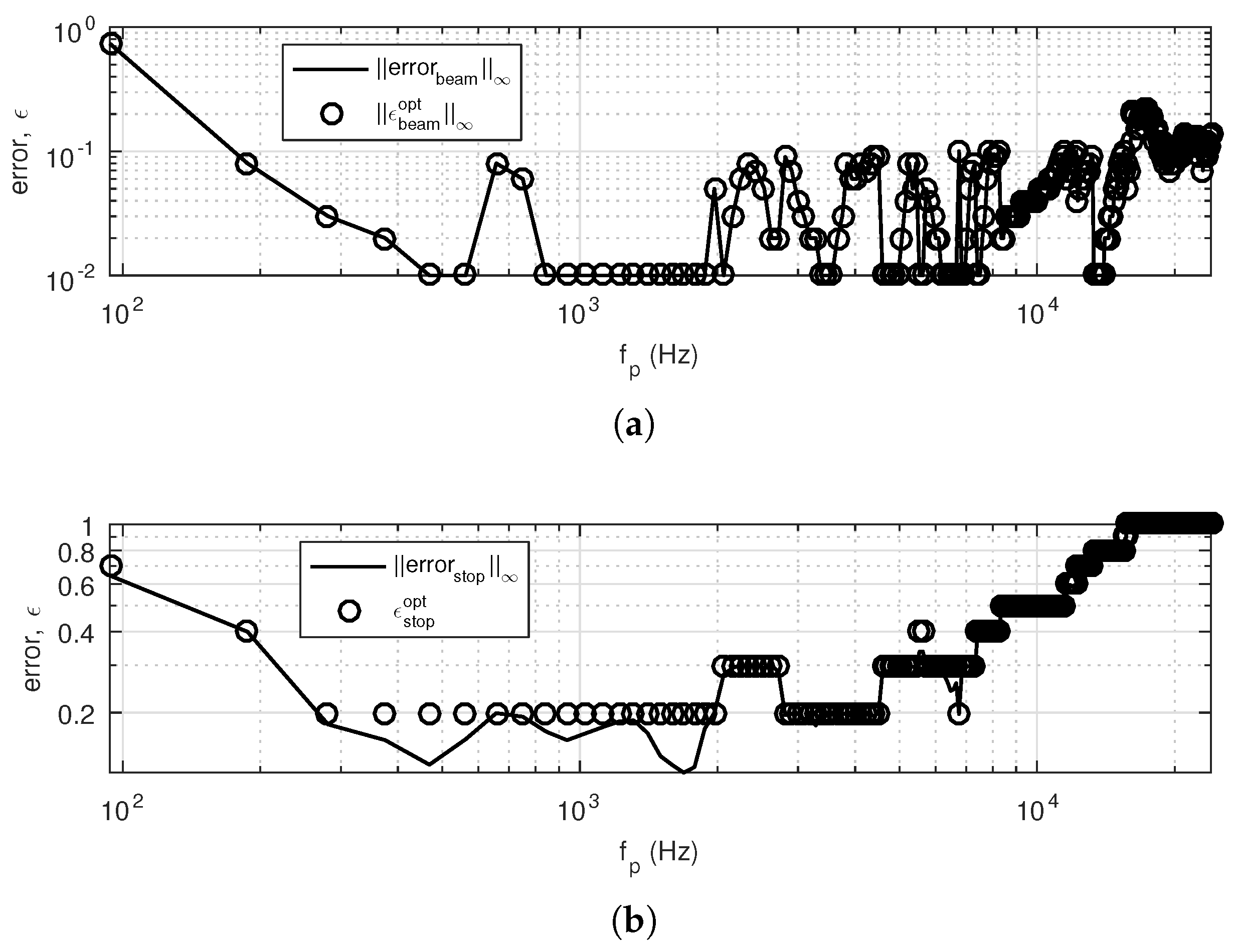
Choosing the correct upper bound for the beam area is difficult: on the one hand, a low upper bound for the beam area leads to a good fit in this area (low ${\mathbf{error}}_{beam}$ values), but to undesired side lobes in the stop area (high ${\mathbf{error}}_{stop}$ values). Consequential, the direct sound will be recorded correctly, but is mixed with the undesired reverberant sound field, which should be ideally suppressed. On the other hand, a high upper bound for the beam area leads to the opposite, a bad fit in the beam area (high ${\mathbf{error}}_{beam}$ values), but low undesired side lobes (low ${\mathbf{error}}_{stop}$ values). The following loop design finds a frequency-dependent optimal upper bound for the beam area, which is a compromise between a good fit in the beam area and only small side-lobes in the stop area.

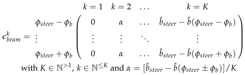
As a first step in the loop design, the upper bound of the beam area is initialized in matrix notation:

(23)

The rows cover the beam area, whereas the columns cover the different iterations of the following loops with k as the counter, where $k=K$ indicates the last iteration. The upper bound starts in the first iteration with ${ϵ}_{beam}^{k=1}=0$ and continues linearly spaced with step size $\alpha$. The step size is designed in such a way that the maximum value of the upper bound of the beam area ${\widehat{b}}_{steer}-\widehat{b}({\varphi }_{steer}\pm {\varphi }_b)$ is reached in overall K steps. Either $\widehat{b}({\varphi }_{steer}-{\varphi }_b)$ or $\widehat{b}({\varphi }_{steer}+{\varphi }_b)$ can be chosen to calculate $\alpha$, since they are equal according to the symmetry of the desired directivity pattern. The upper bound then ends with the difference between ${\widehat{b}}_{steer}$ and ${\widehat{b}}_{beam}$ at the row specific angle. If this difference is reached before the last iteration $(k<K)$, this value will stay till this iteration is reached. This will be the case for every row, except the first and the last one. This procedure ensures that ${\widehat{b}}_{steer}$ stays the maximum value of the directivity pattern.

In contrast to the upper bound of the beam area, the bound of the stop area is initialized as a vector, since there is no angle dependency:

$$\begin{array}{cc}\hfill {ϵ}_{stop}^l& =\begin{array}{ccc}l=1& \cdots & l=L\\ ({\widehat{b}}_{steer}·b_{stop}^{first}& \cdots & {\widehat{b}}_{steer})\end{array}\hfill \\ \hfill & \mathrm{with}L\in {\mathbb{N}}^{>1},l\in {\mathbb{N}}^{\le L}\mathrm{and}{b}_{stop}^{first}\in {\mathbb{R}}^{\ge 0,\le 1}\hfill \end{array}$$

(24)

The entries with the counter l, where $l=L$ indicates the last iteration, correspond to the iterations of the following loops and are linearly spaced. The constant $b_{stop}^{first}$ controls the maximum allowed value of the directivity pattern in the stop area for the first iteration.

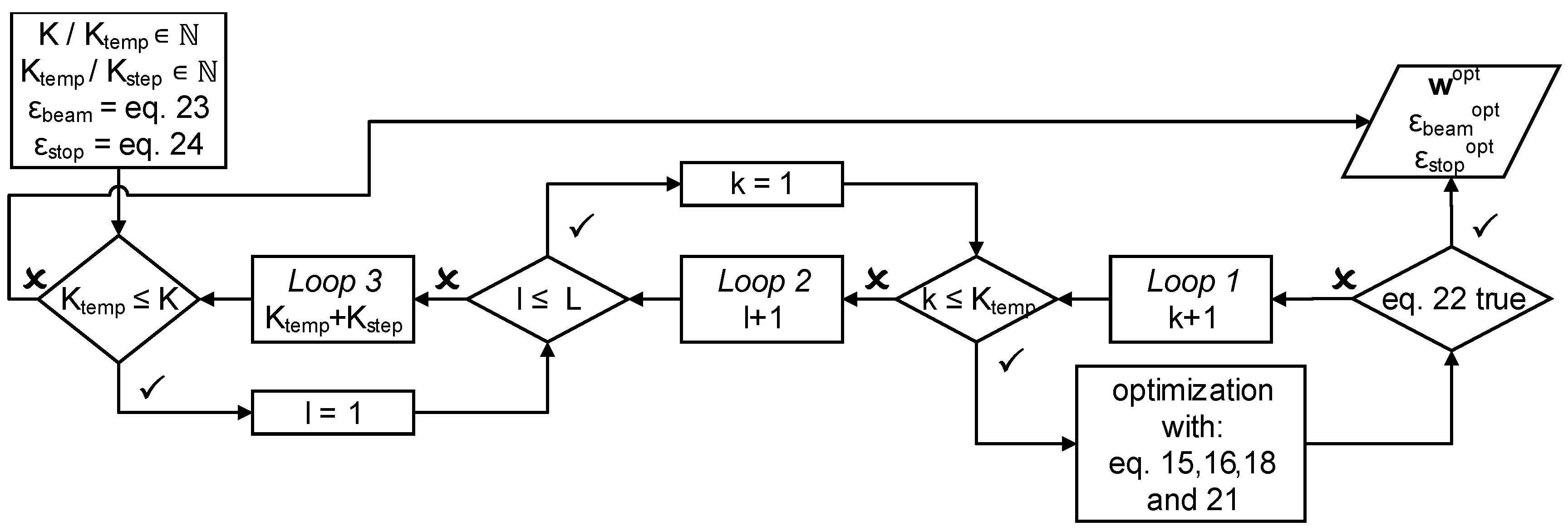
The loop design itself can be seen in Figure 5 and is repeated for every frequency $f_p$, where the constants $K_{temp}$ and $K_{step}$ can be chosen freely so that $K/K_{temp}\in \mathbb{N}$ and $K_{temp}/K_{step}\in \mathbb{N}$, respectively. These two constants regulate the part of the upper bound of the beam area, which is used in the looped optimization process.

The first loop repeats the optimization with the first part of the upper bound of the beam area $(\mathrm{from}{ϵ}_{beam}^{k=1}$ to ${ϵ}_{beam}^{k=K_{temp}\le K})$ till Equation (22) with ${ϵ}_{stop}^1$ is true. A result of the optimization, fulfilling Equation (22), is denoted as valid. If this is not the case, Loop 2 repeats Loop 1 with different upper bounds of the stop area $(\mathrm{from}{ϵ}_{stop}^2\mathrm{to}{ϵ}_{stop}^L)$. If still no valid result is found, Loop 3 increases $K_{temp}$ with the step width of $K_{step}$. The upper bounds, for which the loop design finds a valid solution, are denoted as optimal ${ϵ}_{beam}^{opt}$ and ${ϵ}_{stop}^{opt}$. The filter $\mathbf{w}$, which corresponds to these upper bounds, is also denoted as optimal ${\mathbf{w}}^{opt}$. For the case that $K_{step}$ increases $K_{temp}$ over K $(K_{temp}+K_{step}>K)$, the last $k=K$ calculated result of the optimization is taken as a valid solution.

3. Setup

The following setup is used for the numerical simulations, whose results are described in Section 4 and Section 5. The angular range is discretized into $M=360$ linearly-spaced angles $\{{\varphi }_0=0^{\circ },$${\varphi }_1=1^{\circ },\cdots ,{\varphi }_{359}={360}^{\circ }\}$. The frequency range covers the range of $f_{p=0}=0\mathrm{H}\mathrm{z}$ to $f_{p=256}=24\mathrm{k}\mathrm{H}\mathrm{z}$ generated at a sampling rate of $f_s=48\mathrm{k}\mathrm{H}\mathrm{z}$ using a filter length of 512 samples. This results in $P=257$ linear spaced frequency bins. This frequency range covers the spectral content of music [12] that is to be recorded by these microphone arrays. To obtain impulse responses of the filters, the complex spectrum was mirrored, conjugated and transformed towards the time domain via an ifft.

The microphone array consists of $N=9$ omnidirectional microphones and has a total length of $Length=1\mathrm{m}$. The array design is done with $l_{spread}\approx 35$, so that the smallest microphone spacing $\left(s\right)$ in the center of the array is $s=0.01\mathrm{m}$. Following that, the spatial aliasing frequency can be maximized to a frequency of $f_{al}\approx 17,000\mathrm{H}\mathrm{z}$. For practical reasons, the limitation is set to $s=0.01\mathrm{m}$ to ensure enough space for the microphones. The absolute microphone positions are set as follows (displayed in millimeter precision): $x_{n=-4}=-0.500\mathrm{m}$, $x_{n=-3}=-0.150\mathrm{m}$, $x_{n=-2}=-0.043\mathrm{m}$, $x_{n=-1}=-0.010\mathrm{m}$, $x_{n=0}=0\mathrm{m}$, $x_{n=1}=0.010\mathrm{m}$, $x_{n=2}=0.043\mathrm{m}$, $x_{n=3}=0.150\mathrm{m}$, $x_{n=4}=0.500\mathrm{m}$.

After having specified the microphone positions, the convex functions of the CLSB, shown in Section 2.5, are solved utilizing CVX, a package for specifying and solving convex programs [13,14]. Parts of these convex functions are the WNG constraint and the loop design.

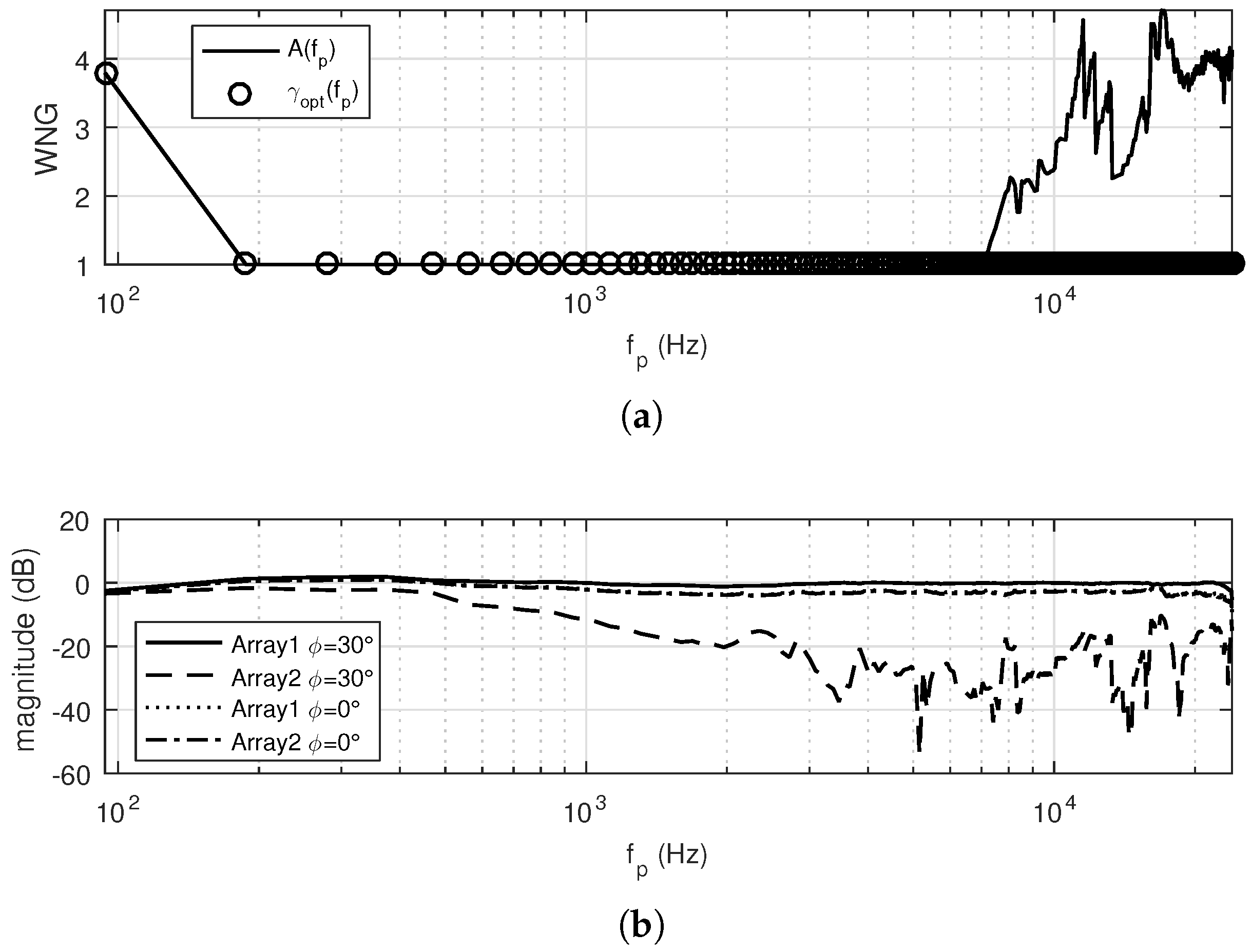
For the WNG constraint, the lower bound $\gamma$ for the WNG $A\left(f_p\right)$ is set up as follows:

$$\gamma \left(f_p\right)=\left\{\begin{array}{cc}5\hfill & \mathrm{for}{f}_p=0\mathrm{H}\mathrm{z}\hfill \\ \mathrm{CSI}\hfill & \mathrm{for}0\mathrm{H}\mathrm{z}<f_p<187.5\mathrm{H}\mathrm{z}\hfill \\ 1\hfill & \mathrm{for}187.5\mathrm{H}\mathrm{z}\le f_p\le f_s/2\mathrm{H}\mathrm{z})\hfill \end{array}\right.$$

(25)

The lower bound starts with $\gamma (f_p=0\mathrm{H}\mathrm{z})=5$ and ends with $\gamma (f_p\ge 187.5\mathrm{H}\mathrm{z})=1$. In the intermediate zone, a Cubic Spline Interpolation (CSI) connects both points. The CSI in the intermediate zone avoids rapid changes of the directivity pattern across frequency below $(f_p<187.5\mathrm{H}\mathrm{z})$. In the high frequency range $(f_p\ge 187.5\mathrm{H}\mathrm{z})$, a lower bound of $\gamma =1$ ensures a robust beamforming design.

For the loop design, the constants are set up as follows:

$$\begin{array}{c}\hfill K=100,K_{temp}=K_{step}=10,\alpha =0.01\mathrm{cf}.\mathrm{Equation}\left(23\right)\hfill \\ \hfill L=9,b_{stop}^{first}=0.2\hfill \\ \hfill {\varphi }_u=10{}^{\circ }\hfill \end{array}$$

(26)

The constants ${\varphi }_b$ and ${\varphi }_{steer}$, as well as the parts of the desired directivity pattern ${\widehat{b}}_{beam}$ and ${\widehat{b}}_{steer}$ are set up according to Section 2.3.

The values of the constants K, $K_{temp}$ and $K_{step}$ are chosen in such a way that Loop 1 scans the beam area from ${ϵ}_{beam}^{k=1}=0$ in steps of $\alpha =0.01$ till ${ϵ}_{beam}^{k=K_{temp}=10}=K_{temp}·\alpha =0.1$. If necessary, Loop 3 increases the value of the upper bound of the beam area according to the value of the constant $K_{step}$ (cf. Section 2.5).

An increase of the value of the constant K leads to an improvement in the beam area (lower $erro{r}_{beam}$ values), because the step size $\alpha$ is smaller. The validity (cf. Section 2.5) of more possible directivity patterns with small $erro{r}_{beam}$ values is checked by the loop design. In fact, to find a valid solution, Loop 2 has to increase ${ϵ}_{stop}$ further than before, which leads to a worsening in the stop area (higher $erro{r}_{stop}$ values). A decrease of the value of the constant K leads consequently to the opposite effect.

An increase of the values of the constants $K_{temp}$ and $K_{step}$ leads to a worsening in the beam area (higher $erro{r}_{beam}$ values), because the first end point of Loop 1 ${ϵ}_{beam}^{k=K_{temp}}$, as well as all of the other ones ${ϵ}_{beam}^{k=K_{temp}+K_{step}+K_{step}+\cdots }$ is now higher. More possible directivity patterns with high $erro{r}_{beam}$ values are checked by the loop design: Loop 2 does not have to increase ${ϵ}_{stop}$ so much than before, because these directivity patterns are in general more likely to be valid. This leads then to an improvement in the stop area (lower $erro{r}_{stop}$ values). A decrease of the values of the constants $K_{temp}$ and $K_{step}$ leads consequently to the opposite effect.

The values of the constants L and $b_{stop}^{first}$ are chosen in such a way that Loop 2 scans the stop area from ${ϵ}_{stop}^{l=1}=0.2$ in steps of $({\widehat{b}}_{steer}-b_{stop}^{first}·{\widehat{b}}_{steer})/(L-1)=0.1$ till ${ϵ}_{stop}^{l=L}={\widehat{b}}_{steer}=1$.

An increase of the value of the constant $b_{stop}^{first}$ and at the same time a decrease of the value of the constant L, preserving the step width of $0.1$ as mentioned earlier, lead to a worsening in the stop area. The start point of Loop 2 is now higher, allowing higher $erro{r}_{stop}$ values from the beginning. It is now easier for Loop 1 to find a valid solution, which leads to an improvement in the beam area. A decrease of the value of the constant $b_{stop}^{first}$ and a coherent increase of the value of the constant L lead to the opposite effect.

Overall, it can be said that a variation of the values of the constants K, $K_{temp}$, $K_{step}$, L and $b_{stop}^{first}$ leads to a changed balance, fulfilling the constraints between the beam and the stop area. For every desired directivity pattern and intended purpose of the microphone array has to be found separately optimal values.

A variation of the value of the constant ${\varphi }_u$ does not significantly change the results in terms of the error in the beam and the stop area. Nevertheless, the value should not be chosen too big to avoid undesired results (very big differences between the obtained and the desired directivity pattern), since there is no control over the directivity pattern in the unconstrained area. The maximum value of ${\varphi }_u$ till there are no undesired results depends in a complex manner on the number of used microphones and the desired directivity pattern.

With the setup shown in Equation (26), we achieved best results in fitting the directivity pattern to the desired one. Different initializations of the constants are also possible, as mentioned before (a detailed analysis of the effect on the results regarding the variation of the constants’ values given in Equation (26) is beyond the scope of this article). Our results are, however, discussed in the following Section 4 and Section 5.

4. Objective Evaluation

The following section is divided into four parts. In Section 4.1, two array designs are compared to each other to show the improvement of the spatial aliasing of a logarithmically-spaced array over a linearly-spaced one. In the second Section 4.2, the new stereo system proposed in this study is compared to the state-of-the-art ones, which utilize two microphones. In the third Section 4.3, the WNG constraint and the frequency response are analyzed. Finally, in the last Section 4.4, the angular constraints, as well as the phase of the directivity pattern are investigated.

4.1. Directivity Index Comparison

The directivity pattern of the logarithmically-spaced array $(l_{spread}\approx 35,s=0.01\mathrm{m})$ is more directive for high frequencies than the one of a linearly-spaced array $(l_{spread}=1,s=0.125\mathrm{m})$ having the same total length of $Length=1\mathrm{m}$. Less reverberant sound is recorded by the first type of array than by the latter one. As a measure, we choose the directivity index $DI$, which is the logarithm of the directivity D [15]:

$$\begin{array}{cc}\hfill D\left(f_p\right)& =\frac{{\sum }_{m=0}^{M-1}{max}_{{\varphi }_m}\left(\right|b(f_p,{\varphi }_m){|}^2)}{{\sum }_{m=0}^{M-1}{\left|b(f_p,{\varphi }_m)\right|}^2}\hfill \\ \hfill DI\left(f_p\right)& =10{log}_{10}\left(D\left(f_p\right)\right)\hfill \end{array}$$

(27)

In fact, Figure 6 shows that the linearly-spaced array has lower $DI$ values for high frequencies $(f_p>1200\mathrm{H}\mathrm{z})$ than the logarithmically-spaced one. This is caused by aliasing effects, as the aliasing frequency for the linearly-spaced array is $f_{al}\approx 1460\mathrm{H}\mathrm{z}$. There is a big drop of the $DI$ values $(DI<7\mathrm{d}\mathrm{B})$ for the logarithmically-spaced array for very high frequencies $(f_p>10,500\mathrm{H}\mathrm{z})$, which is also caused by aliasing effects. The lowest values of the $DI$ for the logarithmically-spaced array are located around the aliasing frequency $f_{al}(\Delta x=s)\approx 17,000\mathrm{H}\mathrm{z}$.

4.2. Comparison Stereo Systems

The necessary phase and/or level differences for a stereophonic recording as mentioned in Section 2.3 can also be obtained by only two microphones. Different angles and distances between these two microphones, as well as different microphone directivity patterns are possible, as described, for example, by the A-B or the X-Y technique [12]. A unified theory of these two-microphone systems for stereophonic sound recording can be found in [6].

Assuming no phase differences, this theory states that a level difference of $\Delta Level=\pm 15\mathrm{d}\mathrm{B}$ determines the left or right lateral shift towards the loudspeakers of a phantom sound source in the playback situation. This level difference is achieved in the recording situation with different angles between two microphones with specific directivity patterns. The angle covering this level difference is called recording angle ${\varphi }_{rec}$. If ${\varphi }_{rec}>{\varphi }_{base}$, the recorded sound scene is compressed in the playback configuration, whereas ${\varphi }_{rec}<{\varphi }_{base}$, the recorded sound scene is expanded [6]. Therefore, we can assume that if we have ${\varphi }_{rec}={\varphi }_{base}$, the recorded spatial properties are the same after playback.

Table 1. The modified directivity index $D{I}_{mod}$ of the state-of-the-art two-microphone stereo systems and the microphone array stereo system described in this study. For the latter one, the desired directivity patterns are used. Only stereo systems with ${\varphi }_{rec}={\varphi }_{base}$ are displayed. This angle constraint avoids angular compression or angular expansion in the playback situation.

Two-Microphone Stereo Systems
Microphone Directivity	Angle between the Microphones ${(}^{\circ })$	${\mathit{DI}}_{\mathit{mod}}$
Figure of Eight	101	$5.95$
Hypercardioid $(\mathrm{back}\mathrm{attenuation}=-6\mathrm{d}\mathrm{B})$	136	$8.29$
Hypercardioid $(\mathrm{back}\mathrm{attenuation}=-10\mathrm{d}\mathrm{B})$	156	$8.7$
Microphone Array Stereo System
$D{I}_{mod}=11.29$ with $b_{mic1}\left({\varphi }_m\right)={\widehat{b}}_{array1}\left({\varphi }_m\right)$ and $b_{mic2}\left({\varphi }_m\right)={\widehat{b}}_{array2}\left({\varphi }_m\right)$

shows the possible microphone directivities and base angles between the microphone pairs.

The microphone array stereo system described in this study records less reverberant sound than these state-of-the-art two-microphone stereo systems. As a measure, we choose a modified definition of the directivity index $D{I}_{mod}$, which is the logarithm of a modified directivity $D_{mod}$, mentioned in Section 4.1:

$$\begin{array}{cc}\hfill D_{mod}& =\frac{{\sum }_{m=0}^{M-1}2{max}_{{\varphi }_m}(b_{mic1}{\left({\varphi }_m\right)}^2)}{{\sum }_{m=0}^{M-1}{b}_{mic1}{\left({\varphi }_m\right)}^2+b_{mic2}{\left({\varphi }_m\right)}^2}\hfill \\ \hfill D{I}_{mod}& =10{log}_{10}\left(D_{mod}\right)\hfill \end{array}$$

(28)

where $b_{mic1}\left({\varphi }_m\right)$ and $b_{mic2}\left({\varphi }_m\right)$ are the directivity patterns of the first and the second microphone, respectively. The modified directivity index includes the sum of the directivity patterns of the two microphones. The modified directivity index considers the angle between these two directivity patterns, which determines the percentage of recorded reverberant sound in addition to the directivity pattern itself. As shown in Table 1, the proposed microphone array stereo system is, in fact, more directive than the two-microphone stereo ones, taking also into account the angle between the two microphone arrays.

4.3. WNG and Frequency Response

The algorithm successfully fits the WNG $A\left(f_p\right)$ to the lower bound $\gamma \left(f_p\right)$ specified in Section 3, as shown in Figure 7a.

This ensures a robust beamforming design. For high frequencies $f_p\ge 7031\mathrm{H}\mathrm{z}$, the algorithm finds even higher WNG values than the lower bound.

Figure 7b shows the frequency response of both arrays according to the configuration that is shown in Figure 3. The responses for both arrays were calculated for a sound source emanating from $\varphi ={30}^{\circ }$ (resulting in a sound source perceived at the location of the left loudspeaker, solid and dashed line) according to Figure 3 and $\varphi =0^{\circ }$ (resulting in a phantom source between both speakers, dotted and dash-dotted line). It can be seen that for $\varphi =0^{\circ }$, the responses of both arrays show a high similarity in terms of level differences and have only minor fluctuations of approximately $\pm 2\mathrm{d}\mathrm{B}$ above $1000\mathrm{H}\mathrm{z}$. Below $1000\mathrm{H}\mathrm{z}$, it can be observed that there is a boost of approximately $3\mathrm{d}\mathrm{B}$, which might be attributed to a violation of a constraint at low frequencies. When the sound source is emanating from $\varphi ={30}^{\circ }$, a flat frequency response can be observed for Array 1 (on axis) with minor fluctuations of approximately $1\mathrm{d}\mathrm{B}$ across frequency. Array 2 shows a considerably lower level, but larger fluctuations. It can be assumed that these fluctuations will not be perceivable because the location of the sound source will be determined by Array 1.

4.4. Beam and Stop Area Constraints

The results of the loop design mentioned in Section 2.5 are shown in Figure 8. This loop design finds a compromise between a good fit in the beam area and low directivity pattern values in the stop area.

For low frequencies $f_p<187.5\mathrm{H}\mathrm{z}$, the directivity pattern is quite omnidirectional $(\parallel {\mathbf{error}}_{stop}{\parallel }_{\infty }>0.2$ and $\parallel {\mathbf{error}}_{beam}{\parallel }_{\infty }>0.1)$, so that Loop 3 has to increase ${ϵ}_{beam}$ to $\parallel {ϵ}_{beam}^{opt}{\parallel }_{\infty }>0.1$. For higher frequencies $f_p\ge 187.5\mathrm{H}\mathrm{z}$, there is a good fit in the beam area $\parallel {\mathbf{error}}_{beam}{\parallel }_{\infty }\le 0.1$ so that Loop 1 and Loop 2 find the ideal upper bound for the beam and the stop area. Overall, it can be said that the best result is found in the frequency range of $281.3\mathrm{H}\mathrm{z}\le f_p\le 1969\mathrm{H}\mathrm{z}$: a good fit in the beam area combined with low directivity pattern values in the stop area $\parallel erro{r}_{stop}{\parallel }_{\infty }\le 0.2$. At high frequencies $(f_p\ge 16,690\mathrm{H}\mathrm{z})$, Figure 8b shows aliasing effects $(\parallel {\mathbf{error}}_{stop}{\parallel }_{\infty }=1)$, which are expected, since the aliasing frequency of the logarithmically-spaced array is $f_{al}(\Delta x=s)\approx 17,000\mathrm{H}\mathrm{z}$.

Figure 9 shows the polar plot of the desired directivity pattern in addition to the absolute value of the directivity patterns of the frequencies $f_p=250\mathrm{H}\mathrm{z}$, $f_p=1000\mathrm{H}\mathrm{z}$, $f_p=4000\mathrm{H}\mathrm{z}$ and $f_p=8000\mathrm{H}\mathrm{z}$. For all frequencies, there is a good fit (a small difference between desired and obtained directivity pattern) in the beam area, as already quantified by Figure 8a. Comparing the side-lobe-levels of the different frequencies, the following can be stated: the side-lobe-level decreases from $f_p=250\mathrm{H}\mathrm{z}$ to $1000\mathrm{H}\mathrm{z}$; there is no big difference in side-lobe-level between $f_p=1000\mathrm{H}\mathrm{z}$ and $f_p=4000\mathrm{H}\mathrm{z}$; the side-lobe-level increases from $f_p=4000\mathrm{H}\mathrm{z}$ to $f_p=8000\mathrm{H}\mathrm{z}$. This analysis is described in a quantified matter in Figure 8b.

Figure 10a allows for a more detailed analysis, as it shows the absolute value of the difference between the directivity pattern and the desired one in the whole angular range $\left|error\right({\varphi }_m,f_p\left)\right|$. The omnidirectional behavior of the directivity pattern up to $f_p=187.5\mathrm{H}\mathrm{z}$ can be also seen there. For higher frequencies, side lobes appear at ${\varphi }_m=\pm 180{}^{\circ }$ and move with increasing frequency into the direction of the beam $-60{}^{\circ }\le {\varphi }_m\le 60{}^{\circ }$. Aliasing effects can be seen in Figure 10a, like in Figure 8b.

In addition to the absolute value of the directivity pattern, the phase $arg\left(b(f_p,{\varphi }_m)\right)$ is represented in Figure 10b.

The directivity pattern is purely real: the phase shows only three possible values $arg\left(b\right)=\{-\mathsf{\pi },0,\mathsf{\pi }\}$ as mentioned in Section 2.3. In the beam area, the phase has, in fact, only values $arg\left(b\right)=0$, which leads to no phase differences between the two arrays in the recording configuration mentioned in Section 2.3.

5. Subjective Evaluation

In this section, the proposed microphone array is subjectively evaluated. For this purpose, a listening experiment was performed, whose results are shown.

5.1. Subjective Evaluation: Localization Accuracy

In order to evaluate the proposed stereophonic-microphone array in terms of localization accuracy when simulating spatially-distributed sound sources, subjective data were obtained in a localization experiment within a real room from listeners. The loudspeaker signals were generated using a single sound source and by simulating the delays between the microphones and the sound source. The optimized filters $w^{opt}$ were applied on each microphone signal to obtain the output signal for the left and right array, which was then played back via the two loudspeakers during the listening experiment. The loudspeaker and array configurations are shown in Figure 3.

The sound sources were placed on virtual locations between $-{30}^{\circ }$ and $+{30}^{\circ }$ in a five degree resolution, resulting in a phantom source stereo image based on intensity-panning between the left and the right loudspeakers. The evaluation took place in a reverberant room with the dimensions $(7.5,7.1,2.97)$ m with a reverberation time of $T_{60}=0.45\mathrm{s}$. The distance between the loudspeakers was $3\mathrm{m}$, and the listeners were seated at the position that created a ${60}^{\circ }$ stereo triangle with the loudspeakers (cf. Figure 3). As a source signal, three short pink noise bursts with a total length of $1.1\mathrm{s}$ were presented to the listeners. The noise covered a frequency rang from $100\mathrm{H}\mathrm{z}$ to $f_s/2$ covering the spectral content of musical signals. Data were obtained from seven listeners, and the 13 source position angles were presented in random order. For each subject, the experiment covered one training session and three measurement sessions. The task of the participants was to indicate the perceived direction between the loudspeaker using indicators placed between the loudspeakers in five degree steps.

5.2. Subjective Evaluation: Results

Figure 11 shows the perceived directions of the subjective evaluation. The dotted line indicates perfect correspondence between the true source location and the perceived location. Circles show the average perceived location in dependence of the simulated source location. As can be seen, there is a rather linear behavior on localization, indicating a mostly precise representation of the presented directions. Exceptions can be observed around $\pm 20$ degrees at which the presented source is perceived more lateral than the simulated source location. The maximum localization error of ≈6 degrees that can be observed can probably be attributed to the target functions that were used to optimize the directivity pattern, which may cause too high level differences when both arrays are used in combination.

6. Discussion and Conclusions

In this study, a new approach for intensity stereophonic recording has been investigated. Guided by the playback situation and its auditory requirements, we decided to postulate a setup consisting of two crossed end-fire microphone arrays and a fitting desired directivity pattern. The difference between the directivity pattern obtained and the one desired was minimized by a superdirective beamforming algorithm. It was based on convex numeric optimization and also contains a frequency-dependent WNG constraint to ensure a robust beamforming design.

In addition to designing the filters of the microphones via beamforming algorithms, we found an ideal array design. This design maximizes the spatial aliasing frequency and also takes practical issues into account, which will appear in an actualization of the arrays. The extent of the microphones demands a particular spacing, also to avoid interferences between them.

A comparison between the new stereo system and the state-of-the-art ones, which use two microphones, has shown that the former has the advantage of less recorded reverberant sound, as it is more directive in the look direction than the latter are. This matches the requirements posed by the recording method proposed in Grosse and van de Par [3], which requires separate dry and reverberated representations of the audio signal. The reverberated sound field can be taken from single microphone signals.

Future research could develop a method to optimize the directivity pattern of both arrays as one system rather than handling them separately. Furthermore, two additional beams pointing into the diffuse field could be introduced for optimization to replace the two microphones placed in that field and to use only the array system.

A final assessment of the proposed recording and playback system needs to run listening tests and investigate the perception of the recording and playback room.

References

1. Berkhout, A.J. A holographic approach to acoustic control. J. Audio Eng. Soc 1988, 36, 977–995. [Google Scholar]
2. Gerzon, M.A. Periphony: With-Height sound reproduction. J. Audio Eng. Soc 1973, 21, 2–10. [Google Scholar]
3. Grosse, J.; van de Par, S. Perceptually accurate reproduction of recorded sound fields in a reverberant room using spatially distributed loudspeakers. IEEE J. Sel. Top. Signal Process. 2015, 9, 867–880. [Google Scholar] [CrossRef]
4. Schroeder, M.R. Statistical parameters of the frequency response curves of large rooms. J. Audio Eng. Soc 1987, 35, 299–306. [Google Scholar]
5. Haeussler, A.; van de Par, S. Theoretischer und subjektiver Einfluss des Aufnahmeraumes auf den Wiedergaberaum. In Proceedings of the 40th DAGA’14 Jahrestagung fuer Akustik, Oldenburg, Germany, 10–13 March 2014. [Google Scholar]
6. Williams, M. Unified theory of microphone systems for stereophonic sound recording. In Proceedings of the 82th Audio Engineering Society Convention, London, UK, 10–13 March 1987. [Google Scholar]
7. Mabande, E.; Schad, A.; Kellermann, W. Design of robust superdirective beamformers as a convex optimization problem. In Proceedings of the 2009 IEEE International Conference on Acoustics, Speech and Signal Processing, Taipei, Taiwan, 19–24 April 2009; pp. 77–80. [Google Scholar]
8. Frost, O.L. An algorithm for linearly constrained adaptive array processing. Proc. IEEE 1972, 60, 926–935. [Google Scholar] [CrossRef]
9. Pulkki, V. Compensating displacement of amplitude-panned virtual sources. In Proceedings of the Audio Engineering Society Conference: 22nd International Conference: Virtual, Synthetic, and Entertainment Audio, Espoo, Finland, 15–17 June 2002. [Google Scholar]
10. McCowan, I.A. Robust Speech Recognition using Microphone Arrays. Ph.D. Thesis, Queensland University of Technology, Brisbane City, QLD, Australia, 2001. [Google Scholar]
11. Corteel, E. On the use of irregularly spaced loudspeaker arrays for wave field synthesis, potential impact in spatial aliasing frequency. In Proceedings of the 9th international converence on Digital Audio Effects (DAFx’06), Montreal, QC, Canada, 18–20 September 2006; pp. 209–214. [Google Scholar]
12. Dickreiter, M.; Dittel, V.; Hoeg, W.; Woehr, M. Handbuch der Tonstudiotechnik, 7th ed.; K. G. Sauer Verlag: München, Germany, 2008; Volume 1. [Google Scholar]
13. Grant, M.; Boyd, S. CVX: Matlab Software for Disciplined Convex Programming, version 2.1. 2014. Available online: http://cvxr.com/cvx (accessed on 18 May 2017).
14. Grant, M.; Boyd, S. Graph implementations for nonsmooth convex programs. In Recent Advances in Learning and Control: Lecture Notes in Control and Information Sciences; Blondel, V., Boyd, S., Kimura, H., Eds.; Springer: New York, NY, USA, 2008; pp. 95–110. Available online: http://stanford.edu/ boyd/graphdcp.html (accessed on 18 May 2017).
15. Kinsler, L.; Frey, A.; Coppens, A.; Sanders, J. Fundamentals of Acoustics; John Wiley and Sons, Inc.: New York, NY, USA, 2000. [Google Scholar]
Figure 1. Recording and playback configuration with a processing stage in between to maintain the acoustical perception of a recording room. The microphone ( C ) records the direct sound, which is played later by two conventional loudspeakers, whereas the two microphones ( B l ) and ( B r ) record the reverberant sound field, which is played later by two dipole loudspeakers. Figure reproduced with permission from [3], Copyright IEEE, 2015.
Applsci 07 00541 g001
Figure 2. Microphone array receiving a signal with frequency f and angle of incidence ϕ . The incoming wavefront is captured with a microphone n, modified with the respective filter w n and, at the end, summed up to form the directivity pattern b ( f , ϕ ) .
Applsci 07 00541 g002
Figure 3. The stereophonic recording configuration is based on the playback one. Recorded level and phase differences with the two end-fire microphone arrays generate a phantom source between the two loudspeakers in the playback configuration. The signal emitted from Loudspeaker 1 has the level L e v e l 1 and the phase p h a s e 1 . The signal emitted from Loudspeaker 2 has the level L e v e l 2 and the phase p h a s e 2 . (a) Typical stereophonic playback configuration [9]; (b) proposed stereophonic recording configuration with sketched microphone positions. The absolute microphone positions are shown in Section 3.
Applsci 07 00541 g003
Figure 4. Different spatial areas in the directivity pattern optimization problem. The steering angle ϕ s t e e r , the beam area ϕ b e a m (indicated by horizontal hash lines), an area without any constraints ϕ u n c o n s t r a i n e d (indicated by crossed hash lines) and the stop area ϕ s t o p (indicated by vertical hash lines).
Applsci 07 00541 g004
Figure 5. Loop design to determine the optimal filter, as well as the optimal upper bound for the beam and the stop area.
Applsci 07 00541 g005
Figure 6. Directivity index D I ( f p ) of a linearly-spaced array ( l s p r e a d = 1 , s = 0 . 125 m ) (dashed line) and the logarithmically-spaced one ( l s p r e a d 35 , s = 0 . 01 m ) (solid line) with the same total length of L e n g t h = 1 m .
Applsci 07 00541 g006
Figure 7. (a) White Noise Gain (WNG) A ( f p ) , as well as the lower bound for the WNG γ ( f p ) across frequency; (b) shown are frequency responses of both arrays for two sound sources emanating from ϕ = 30 and ϕ = 0 according to the configuration illustrated in Figure 3.
Applsci 07 00541 g007
Figure 8. The difference between the simulated directivity pattern and the desired one ( e r r o r ) in the beam (a) and the stop (b) area, as well as the corresponding upper bounds of both areas as function of the frequency.
Applsci 07 00541 g008
Figure 9. Polar plot of the desired directivity pattern (grey markers) and the absolute value of the obtained directivity patterns of the frequencies f p = 250 H z (solid line), f p = 1000 H z (dashed line), f p = 4000 H z (dashed-dotted line) and f p = 8000 H z (dotted line).
Applsci 07 00541 g009
Figure 10. The difference between the directivity pattern and the desired one | e r r o r ( f p , ϕ m ) | (a), as well as the phase of the directivity pattern arg ( b ( f p , ϕ m ) ) (b).
Applsci 07 00541 g010
Figure 11. Illustrated are the mean-values of the perceived angle of incidence with the standard deviation across seven participants’ means. The x-axis represents the simulated angle of incidence ϕ of the presented noise sources. The dotted line indicates a perfect match between simulated and perceived localization.
Applsci 07 00541 g011