1. Introduction
An excessiverise in temperature due to heat generation during the cutting process is an important issue that not only accelerates tool wear but also affects machining accuracy and surface quality of the finished workpieces [
1]. Therefore, the research on active control of cutting temperature via promotion of heat-dissipation is indispensable for a highly reliable machining process. Wet machining using different kinds of cutting fluids is a most widely used technique to maintain the cutting temperature below some specified optimal cutting temperatures [
2]. However, the excessive use of cutting fluids becomes a major problem owing to some associated economic, environmental and health concerns [
3]. Dry machining can be considered as a feasible approach to eliminate the use of cutting fluids because of low processing cost and soft ecological hazard [
4]. Compared with wet machining, dry cutting shows some superiority such as lower thermal shock and improved useful life of cutting tools, however, the machining friction and the cutting temperature during dry machining are usually greater than those of wet machining. Temperature has an impact on tool wear, thus it is important for the cutting process [
5,
6]. Aiming at achieving better temperature reduction performance in dry machining process, researchers have proposed a variety of methods and achieved some meaningful results. Jerold [
7] and Tazehkand [
8] investigated the utilization of CO
2 and liquid nitrogen as cooling media to reduce the cutting temperature and reported good improvements. On the other hand, heat pipe cooling is also a widely utilized method to improve cutting performances and has attracted significant attentions [
9,
10].
Regarded as an indirect cooling system (ICS), research on the internal cooling system has already been a hot topic in industry because of its convenient installation for conventional machine tools. Since the initial description of this type of cooling system in the 1970s, a variety of improvements have been proposed. Ferri designed an internally cooled cutting tool consisting of a modified cutting insert, cooling adapter accommodating micro-channel, and tool-holder with inlet and outlet ports [
11]. Minton created a modified tool-holder with an internally cooled tool to enhance the heat transfer [
12]. In these two studies, pyrometers were employed to monitor the rise of cutting temperature and evaluate the enhancement of cooling effect. Sun presented an enclosed internal cooling circuit in the support seat [
13], and in his study, a thermal imager was employed to measure cutting temperatures in the machining process. Among the above reported literature, research on ICS mainly focuses on modifications of tool-holder forms, support seat or the insert. These methods above can indeed be improved, however they usually require additional supply devices that inevitably increase the complexity of the machining tool or modify the machine tool structure, significantly limiting industrial applications.
Considering the pros and cons of the above cooling methods, in this paper, a novel independent cooling system based on an internal cooling fluid channel is devised and applied to promote heat dissipation during cutting process. A distinct advantage of this novel ICS lies in its simplified mechanical structure and high heat dissipation-promoting performance. Compared with traditional ICS, the proposed independent internal cooling system needs only limited modification for the cutting component and the cooling media can also be replaced by the existing refrigerating system. The heat–energy balance equations of the cooling structure are established to evaluate the cutting temperature. Temperature fields on the rake face and on the flank face were simulated on the numerical platform of Ansys CFX (12.1, ANSYS, Inc., Canonsburg, PA, USA, 2009). Moreover, turning tests were carried out to verify the validation of the numerical model which was previously put forward. In the experiments, turning tests were performed on workpieces made of medium carbon steel of the grade 1045 (the carbon content in the steel is 0.45% according to technical standard provided by the American society for testing and materials). The experimental results demonstrated the effectiveness of the novel independent ICS and the improved cooling performance.
2. Design of Cutting Tool with Independent Internal Cooling Structure
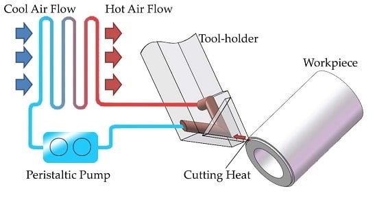
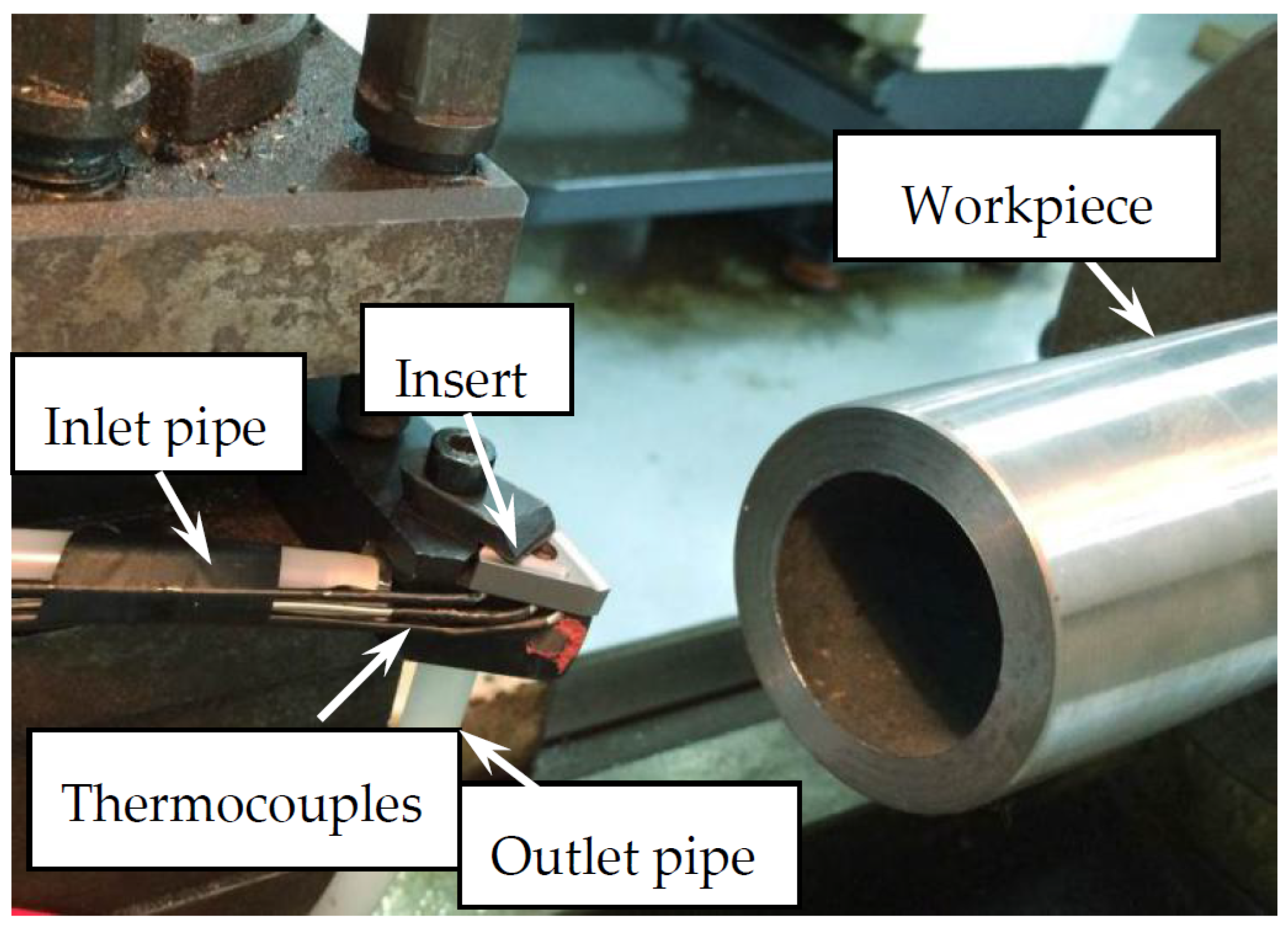
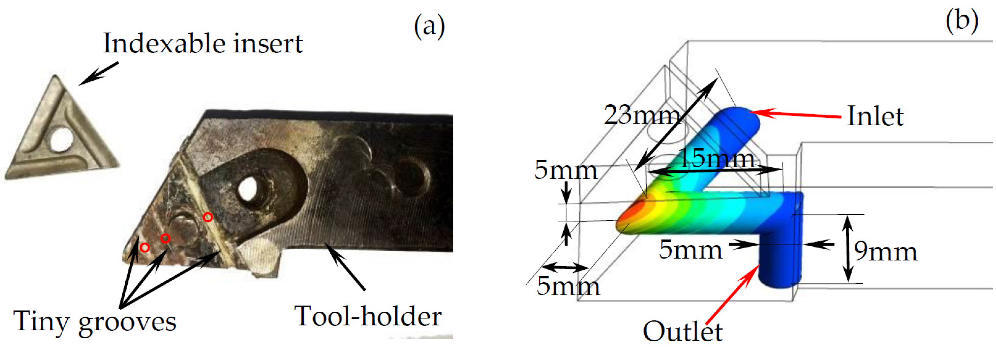
The internal cooling cutting tool system, based on a novel internal channel and designed to enhance heat transfer, is presented in
Figure 1. A carbide insert (YT14 (ISO P20) 31303C, Zhuzhou Cemented Carbide Cutting Tools, LTD, Zhuzhou, Hunan, China) was used in this research. A tool-holder (90° 20W3K13, Taizhou Tingfeng CNC Tools Co., LTD, Taizhou, Zhejiang, China) was modified with a connected V-shaped channel created inside. The cooling liquid was pumped with a peristaltic pump through the V-shaped channel and forming a closed internal cooling circuitry in the tool-holder. Three tiny grooves were machined by the electrospark wire-electrode for placing the thermocouples for temperature measurement. Three temperature measure points were marked with red circles in
Figure 1a. V-shaped channel (colored part) and its design parameters are described in
Figure 1b, different colors represented the temperature distribution in the CFX simulation process. The thermal flux from the machining process is conduced into the insert and then permeates into the air and the channel. The area of high values of thermal flux in the field is extremely localized because of the relatively small area of the tool-chip interface. Therefore, practical cooling channels of high performance are supposed to be placed around the insert rake face in a manner as closed as possible.
3. Numerical Analysis of the Thermal Performance
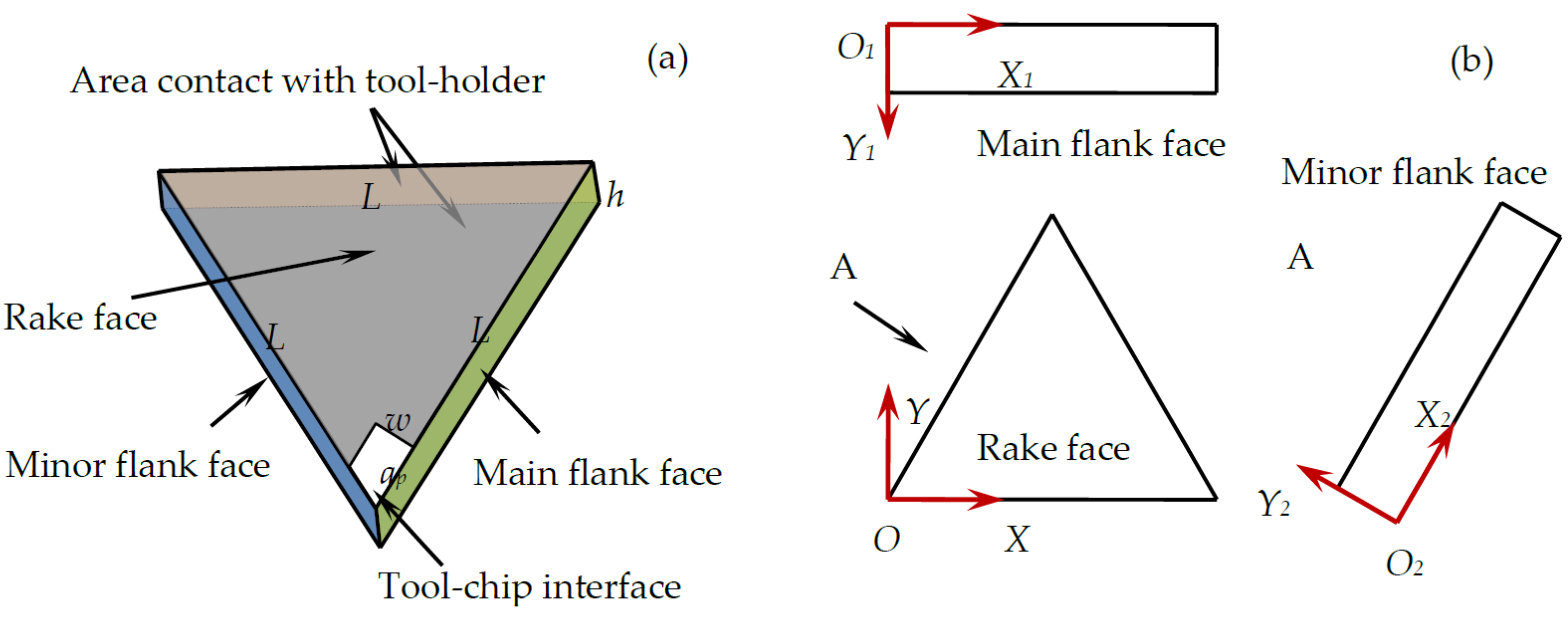
Figure 2 illustrates the triangle indexable insert and the definition of the coordinate systems in this research. The variable
L is the side length of the equilateral triangle; and the variable
is referred to as the thickness of the insert. The area marked by white rhombus in
Figure 2a indicates the tool-chip interface in the machining process. Let
be the cutting width and
be the depth of cut. Therefore, the cutting area can be presented as
. The tool-chip contact area is very small compared with the insert surface. Previous research showed that the maximum cutting temperature is located at a position that is near the center of the tool-chip contact area. For simplicity, the tool-chip contact face was assumed as a uniform temperature distribution area [
14]. There are three different coordinate systems, which are defined as
S(
XOY),
S1(
X1O1Y1) and
S2(
X2O2Y2).
S(
XOY) is the coordinate system established on the rake face;
S1(
X1O1Y1) denotes the main flank face of the insert; and
S2(
X2O2Y2) stands for the minor flank face. The three distinct coordinate systems coincide at the same origin that is located at the tool tip.
3.1. Energy Balancing
The heat–energy balance equations of the insert system can be written as follows [
14,
15]:
where all the physical meanings of the variables in Equation (1) are listed in
Table 1.
According to Newton’s law of heat transfer, Equation (1) can be rewritten as below:
where
denotes the heat transfer coefficient of the area exposed to the air, and the quantities
,
and
denote temperature of the rake face, the main flank face and the minor flank face, respectively.
As can be seen in the above, an essential problem of applying Equation (2) lies in that there are many unknown quantities (, , , , , ) that are difficult to be determined. Values of these unknown quantities will be explained and specified explicitly in detail in the following sub-sections.
3.2. Approximation of the Temperature Fields
Calculating the temperature fields on the rake face, the main flank face and the minor flank face is indispensable for evaluating the quantity of heat that dissipates into the air. In this work, the temperature fields of these surfaces were obtained via a numerical simulation platform of Ansys CFX. In order to acquire the temperature field distribution, finite element orthogonal simulation is performed to acquire the relationship of cutting depth and contact area temperature when cooling liquid velocity was fixed in 80 mL/min. Assume that the generated heats in cutting process are all dissipated through chip, tool and workpiece. Select the working fluid as water. The interface between internal channel and tool-holder is set as the “Fluid–Solid Interface”. The interface between insert and tool-holder is set as the “Solid–Solid Interface”. The simulation parameters are listed in
Table 2.
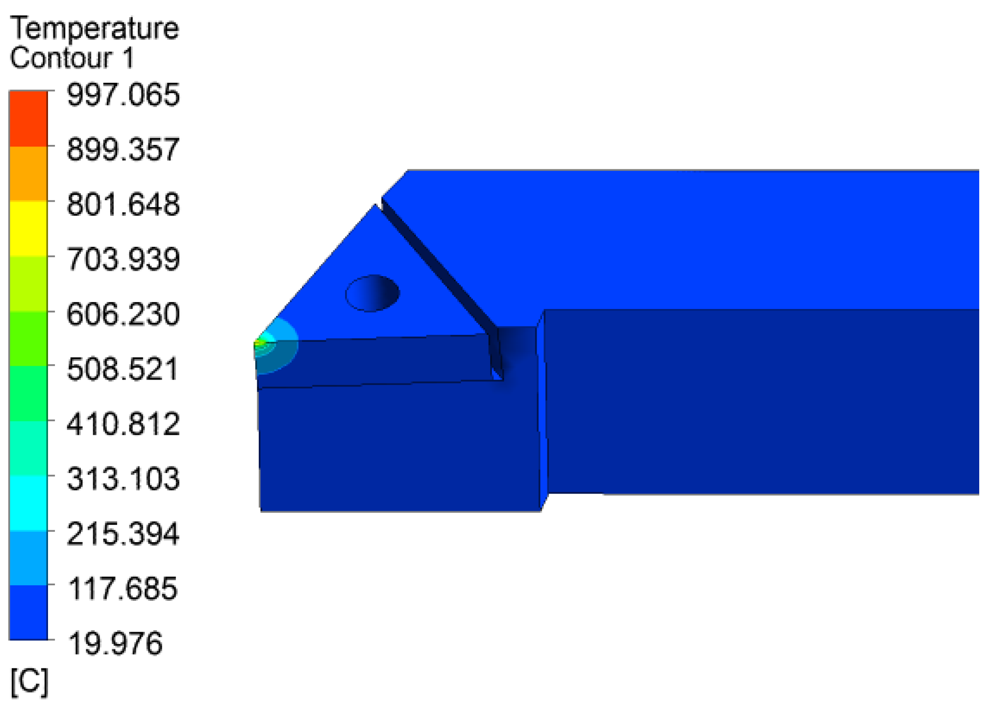
Figure 3 illustrates the tool temperature contours at one experimental point. The contact area was set as 1.0 mm × 0.1 mm. The temperature on the contact area was 1000 °C. It can be inferred from
Figure 3 that the maximum value and the greatest gradient of the temperature fields on the three surfaces occur simultaneously at the tool nose. In order to summarize the temperature field mathematically, fitting methods will be used in this study.
3.2.1. Temperature Filed on the Rake Face
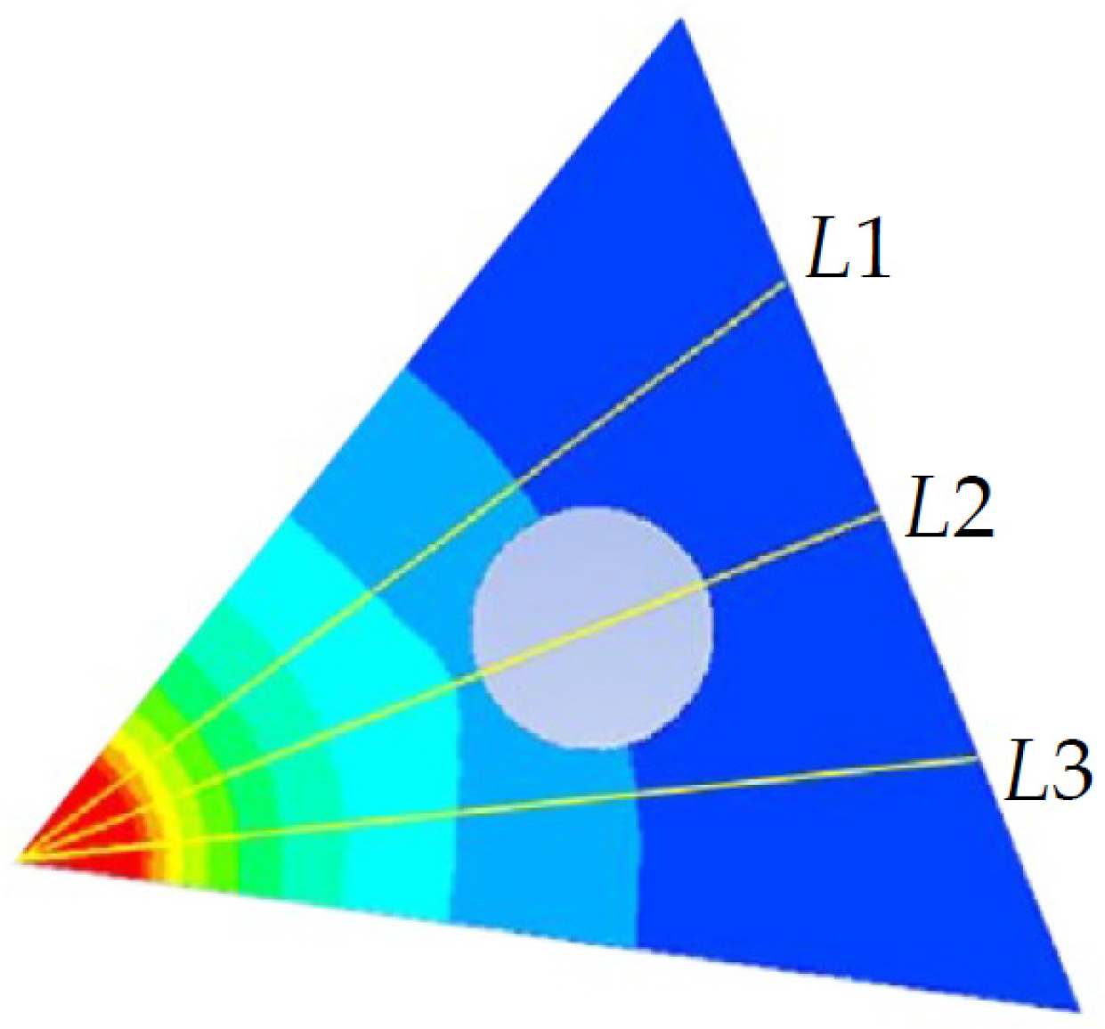
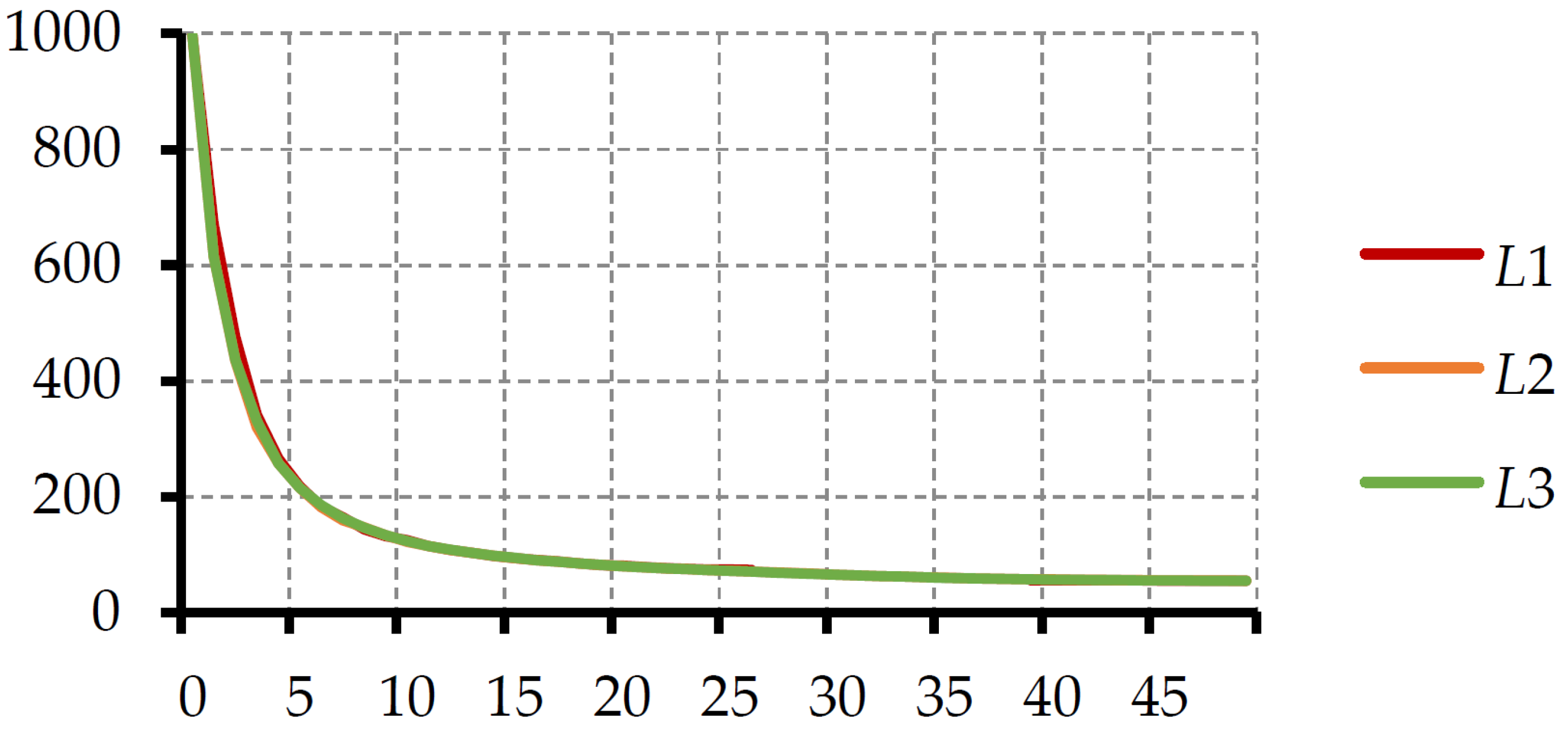
Figure 4 shows the temperature field on the rake face, where different colors represented the temperature distribution in the CFX simulation process. To ensure proper fitting of the field, three straight line paths, which are denoted by
, were deployed to probe the temperatures on them. The temperature distributions along the three straight lines are shown in
Figure 5.
Figure 5 shows their temperature distribution have little difference. Considering the characteristics of the temperature distributions, negative exponential function is suitable to illustrate it.
Orthogonal experiment is carried out to fit the simulated temperature field. As such, the temperature field on the rake face can be expressed as:
3.2.2. Temperature Filed on Main Flank Face
The temperature field on the main flank face is shown in
Figure 6, where different colors represented the temperature distribution in the CFX simulation process. Following the above approach, the temperature field can be also approximately expressed via similar function models. Temperatures of the points located far away from the heat source are also assumed to be equal to the ambient temperature
. Therefore, the temperature field on the main flank face can be approximately expressed as:
3.2.3. Temperature Filed on Minor Flank Face
Similar to the distribution of the temperature field on the rake face and that on the main flank face, the approximate fitting of the temperature field on the main flank face can also be summarized as:
3.3. Thermal Resistance Analysis
Two factors contribute significantly to the actual thermal resistance, that is, the equivalent thermal resistance between the channel and interface, and the contact resistance between the insert and the tool-holder.
3.3.1. Tool-Holder and Internal Fluid Channel
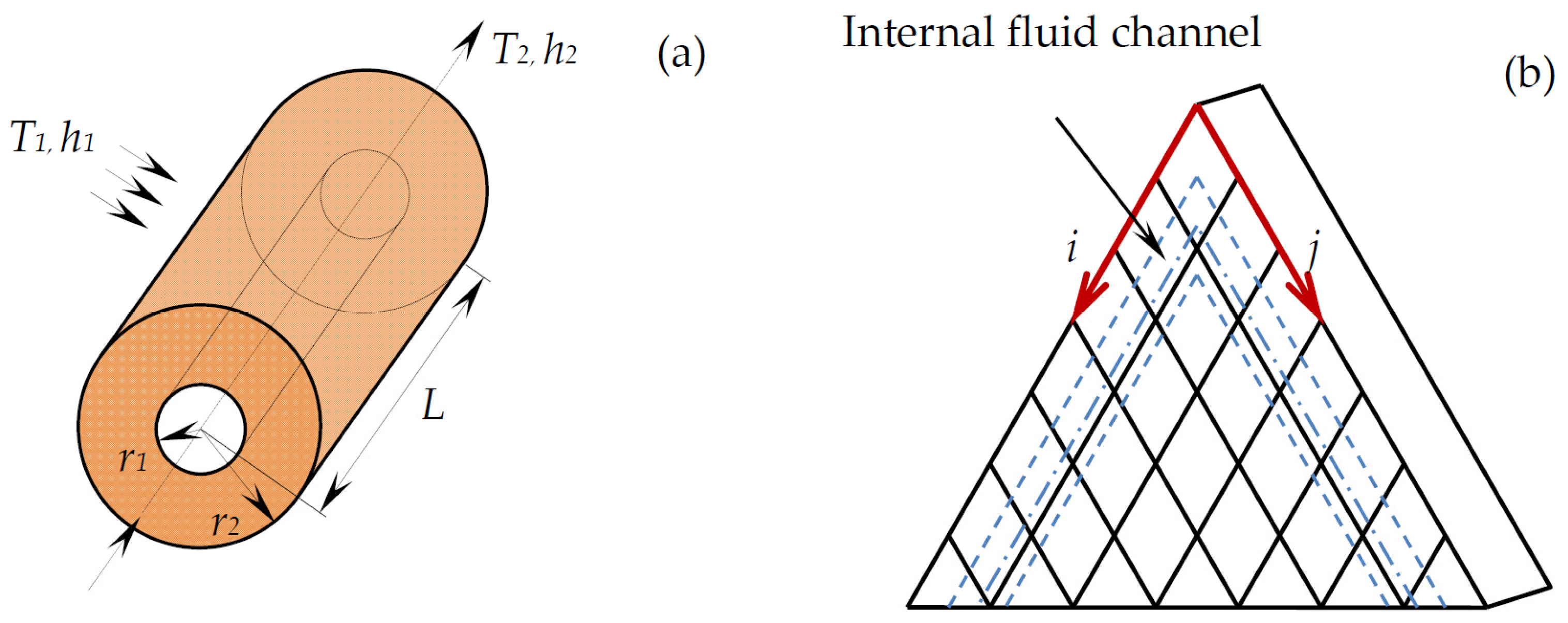
The proposed independent internal cooling structure, composed of connected cooling fluid channels, can be regarded as a novel form of cylindrical cooling systems (CCS). CCS is often theoretically characterized by temperature gradients in radial directions. As shown in
Figure 7a, the cylindrical wall separates two fluids of different temperatures. According to Newton’s law of heat transfer, the thermal resistance for radial conduction in a cylindrical wall is expressed as [
16]:
where
r1,
r2 are the radius of the inner surface and outer surface respectively;
L is the length of the channel; and
k is thermal conductivity.
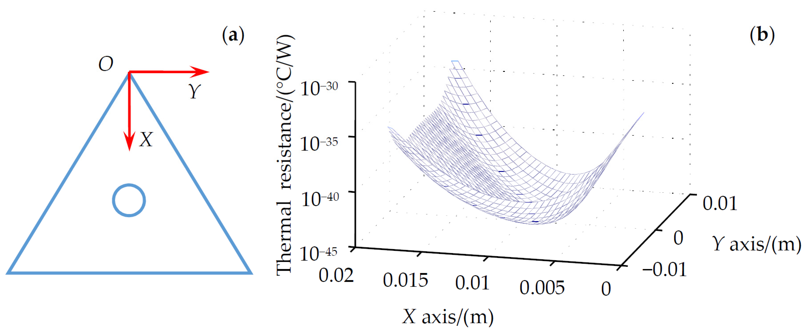
We divide the interface surface between the insert and the tool-holder into different elements, as shown in
Figure 7b. The connected internal fluid channels are located within the tool-holder and deployed according to the geometric shape of the tool-holder such that they are very closed to the interface marked by the blue dash lines in
Figure 7b. The thermal resistance between the unit
can be regarded as the parallel connection of every internal fluid channel unit. Therefore, the thermal resistance of unit
is presented written as:
where
is the thermal resistance between the
kth internal fluid channel unit and unit
of the interface between the insert and the tool-holder, and
n is the number of the unit.
From the above results, the thermal resistance distribution can be calculated to validate the enhancement of the heat transfer process.
Figure 8 shows the thermal resistance at different locations on the interface in this research. A total of 840 points that are evenly spaced are sampled from the interface.
Figure 8a is the coordinate definition diagram, with the origin located in the tool nose. The minimum thermal resistance located on the center of the interface indicates good heat dissipation performance in this interface.
The Reynolds number is defined as the ratio between the inertia force and the viscous force [
17,
18], utilized to characterize different flow regimes within a similar fluid such as laminar or turbulent flow [
19]. The Reynolds number is defined as:
where
is a scale of variation of velocity in a length scale
L;
v is the velocity of flow;
d is the diameter of the channel and
is the liquid viscosity. Therefore, the convection coefficient can be written as:
where
represents the thermal conductivity of the fluid;
is the Nusselt number [
20]; the constants
C and
m can be chosen from references [
20,
21];
is the Prandtl number; and
l is the characteristic length.
The thermal circuit can be constructed on the basis of the fact that the thermal resistance is associated with the heat conduction between the insert and the tool-holder. The equivalent thermal resistance between the tool-holder and the internal fluid channel can be acquired as:
Therefore, on the interface between tool-holder and internal fluid channel, the heat flow can be expressed as:
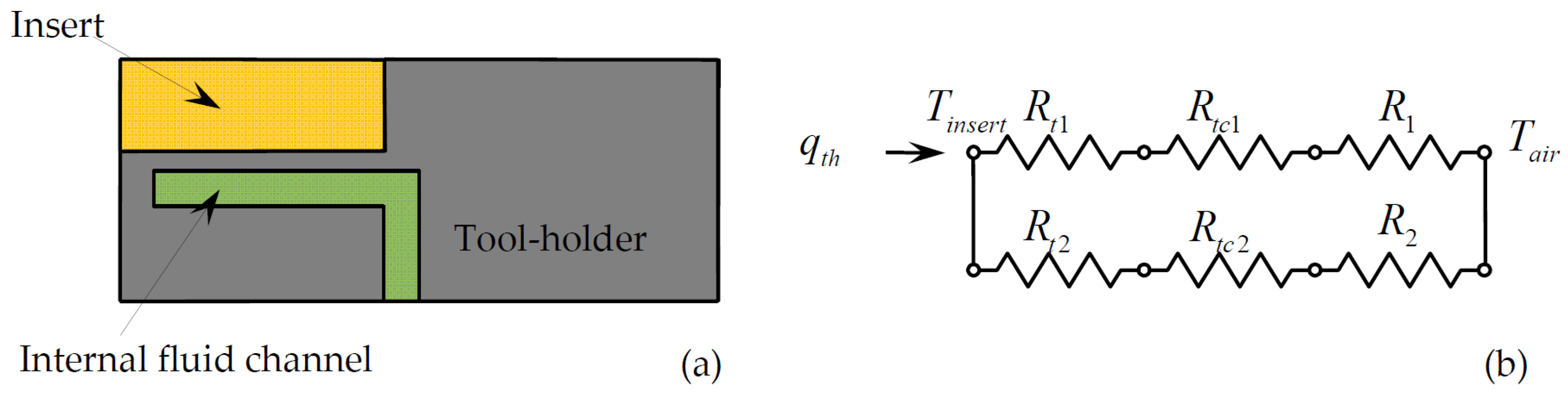
3.3.2. Interface between Insert and Tool-Holder
Owing to the existence of surface roughness, there is a temperature drop across the interface between the insert and the tool-holder. Generally, the associated contact resistance is influenced by the roughness level of the mating surfaces and the joint pressure [
16,
22]. Treating insert and tool-holder as one-dimensional, the sketch is presented in
Figure 9a.
The equivalent thermal resistance between the insert and the tool-holder can be regarded as the parallel circuits of the resistances through different directions (
Figure 9b). Therefore, the equivalent thermal resistance is written as:
where
Rt1,
,
R1,
R2 are the thermal resistances associated with the process of heat conduction between the insert and the tool-holder. These quantities can be calculated using the formula
R = 1/(λ
A1/
d +
hA2), where
is the thermal conductivity,
d is the thickness of a part,
A1 is the area of cross-section of a part,
A2 is the area of the surface exposed to the air, and
h is the heat transfer coefficient of the area contact with air.
Rtc1,
Rtc2 are the thermal contact resistance between the insert and the tool-holder and can be calculated using
Rtc = d/(λ
wAw) where
d is the thickness of the layer,
is the contact area, and λ
w is the thermal conductivity of water.
Therefore, on the interface between the insert and the tool-holder, the heat flow can be expressed as:
3.4. Average Temperature of the Insert
Tinsert is an indispensable parameter required by Equation (2), while the main focus in this research is the tool–chip interface. Therefore, it is significant to determine the instinct relationship. Dividing the insert into multiple small pieces from the different function faces, the average temperature of the insert can be regarded as the weighted mean temperature of these multiple small pieces. As such, the volume average temperature of the insert temperature can be written as:
where
denote the area of different function faces.
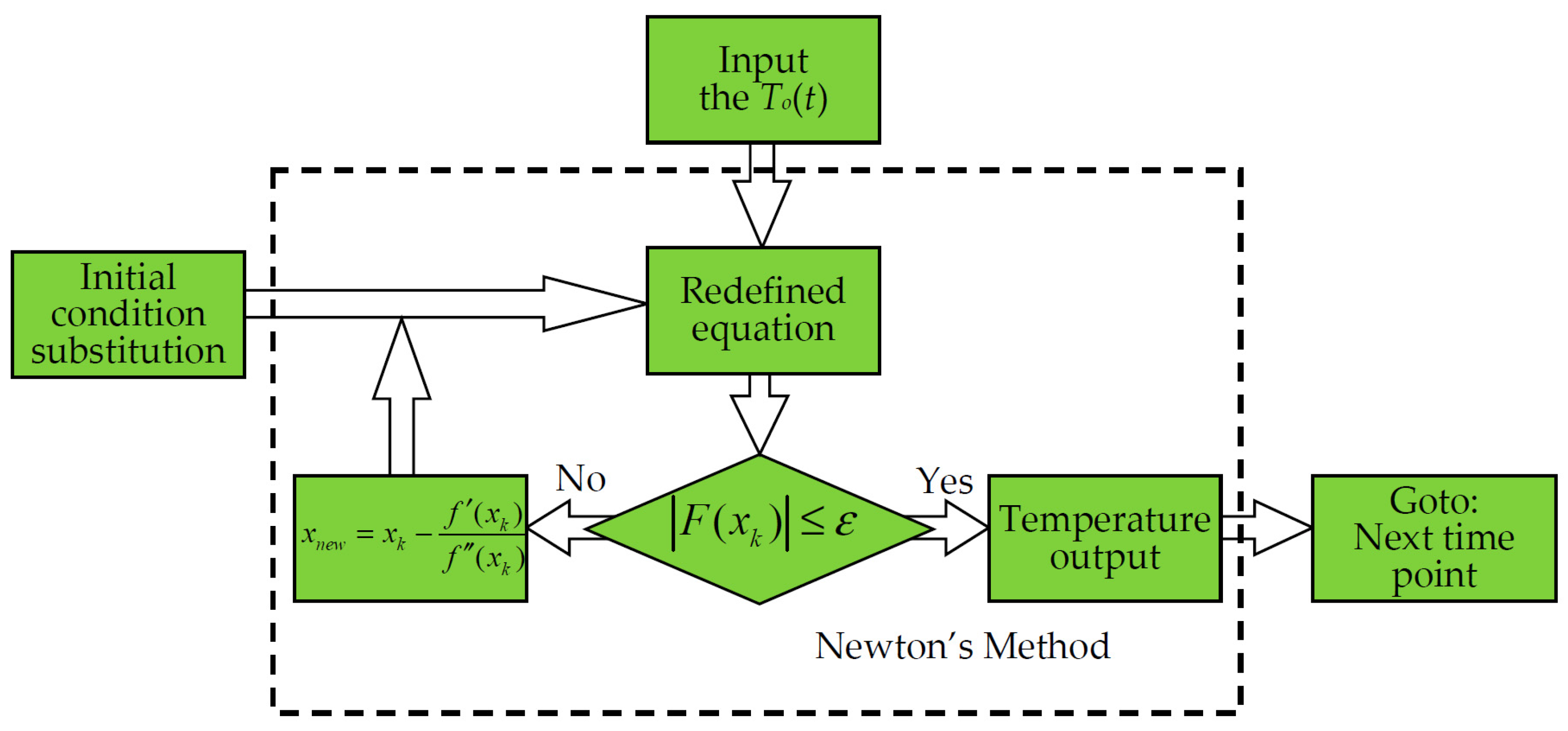
3.5. Iterative Algorithm for Computing Cutting Temperature
On the basis of the above sub-sections, all the parameters in the energy equation shown in Equation (1) are explicitly specified. However, the derived equation is still very difficult to be evaluated analytically. Considering the available initial conditions given by
Tc(0) =
Tair and
, we employ numerical analysis techniques to solve the equation conveniently. The flowchart of the solving algorithm is presented in
Figure 10.
The numerical equation to be solved in the algorithm can be redefined as:
Initial values of the above equation are determined based on the empirical guess for the height of the tool–chip interface temperature. Substituting this temperature into the equation, new values of
are obtained. A tolerance error of a small value is allowed as the convergence criterion for the Newton’s method [
23]. The stopping criterion of the iterative algorithm is that
, where
is the numeric tolerance very close to zero, which controls the numerical accuracy as well as the convergence of the iterations. After evaluating all the temperature field in each iteration, the dynamical temporal evolution of the temperature field on the tool–chip interface, as well as its temperature field at specific time instance, are acquired conveniently.
3.6. Measure Point Temperature
As presented in
Section 3.2, the temperature fields of these surfaces can also be calculated on the simulation platform of Ansys CFX.
3.6.1. Temperature Field along the Insert Thickness Direction
To fit the temperature field along the direction of insert thickness, a path of straight line is deployed to probe the temperatures. Owing to the comparatively consistent temperature distribution along the radial directions from the vertex of the interface, the path temperature along the insert thickness direction can be expressed as:
where
l is the distance between the measure point and the tool tip.
3.6.2. Temperature Field on the Interface of Insert and Tool-Holder
Figure 11 shows the temperature distribution of the interface of insert and tool-holder, where different colors represented the temperature distribution in the CFX simulation process. The temperature distribution on the interface between the insert and the tool-holder can be expressed as:
where
is the maximal temperature of the interface. Substituted the coordinate of measure point in Equation (17) the measure point temperature can be easy to acquire.
Based on the calculated temperature field on the tool-chip interface and the mathematical deductions illustrated above, temperatures of the three measure points can be acquired.
5. Conclusions
In this paper, we proposed a novel independent internal cooling system. The novel type of ICS adopts closed internal fluid channels in the tool-holder for promoting heat dissipation during dry cutting processes. We derived the heat–energy balance equations of the insert system and Ansys CFX was employed to make numeric simulation of the actual temperature fields. The model of lumped parameter and Newton’s iterative method were employed to solve the equation. A cutting trial on the lathe was presented to validate the established model and a new type of mean filter based on EMD was proposed to acquire the smooth signal. Major conclusions of this work can be summarized as below.
- (1)
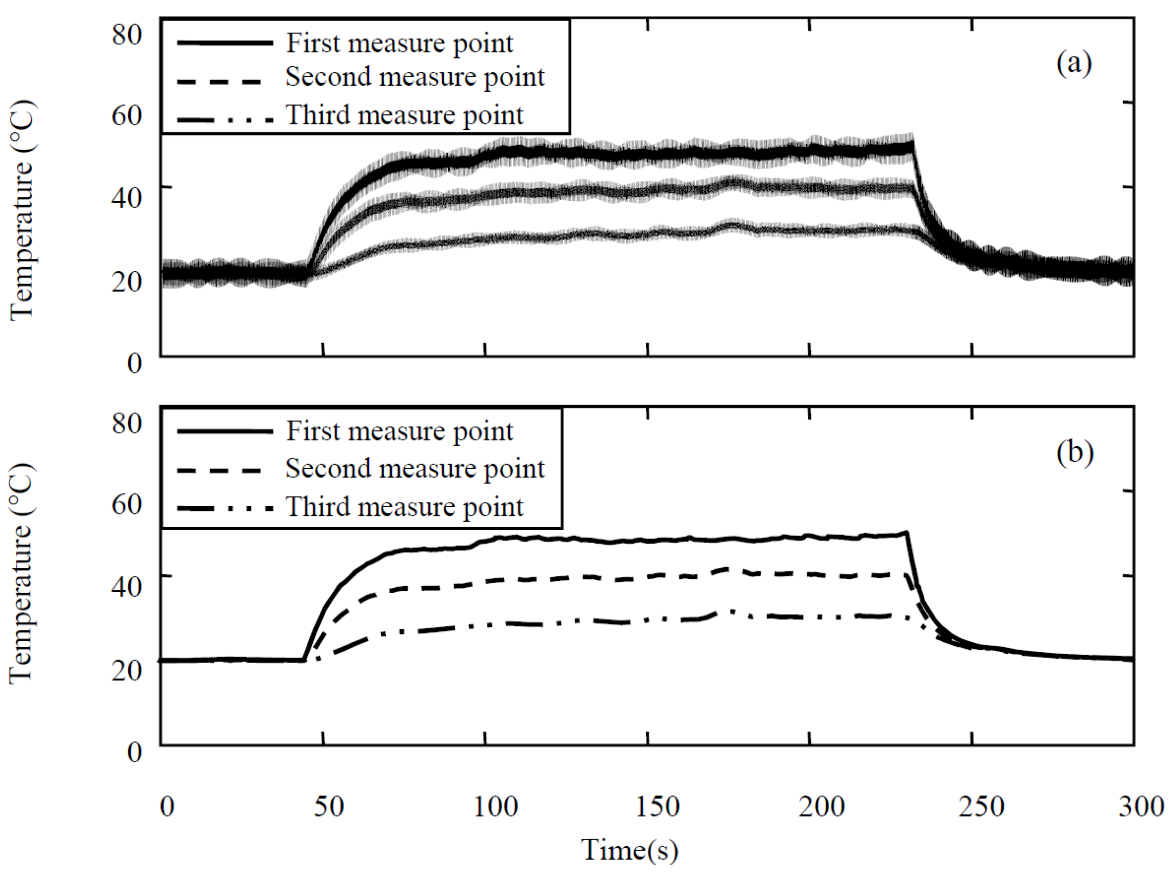
The internal fluid channel could be utilized as an effective way to suppress excessive temperature rise on the tool–chip interface. Compared with conventional dry cutting, the maximal temperature on the measured point was decreased by almost 30% after using the internal fluid channel, independent of supplementary accessories.
- (2)
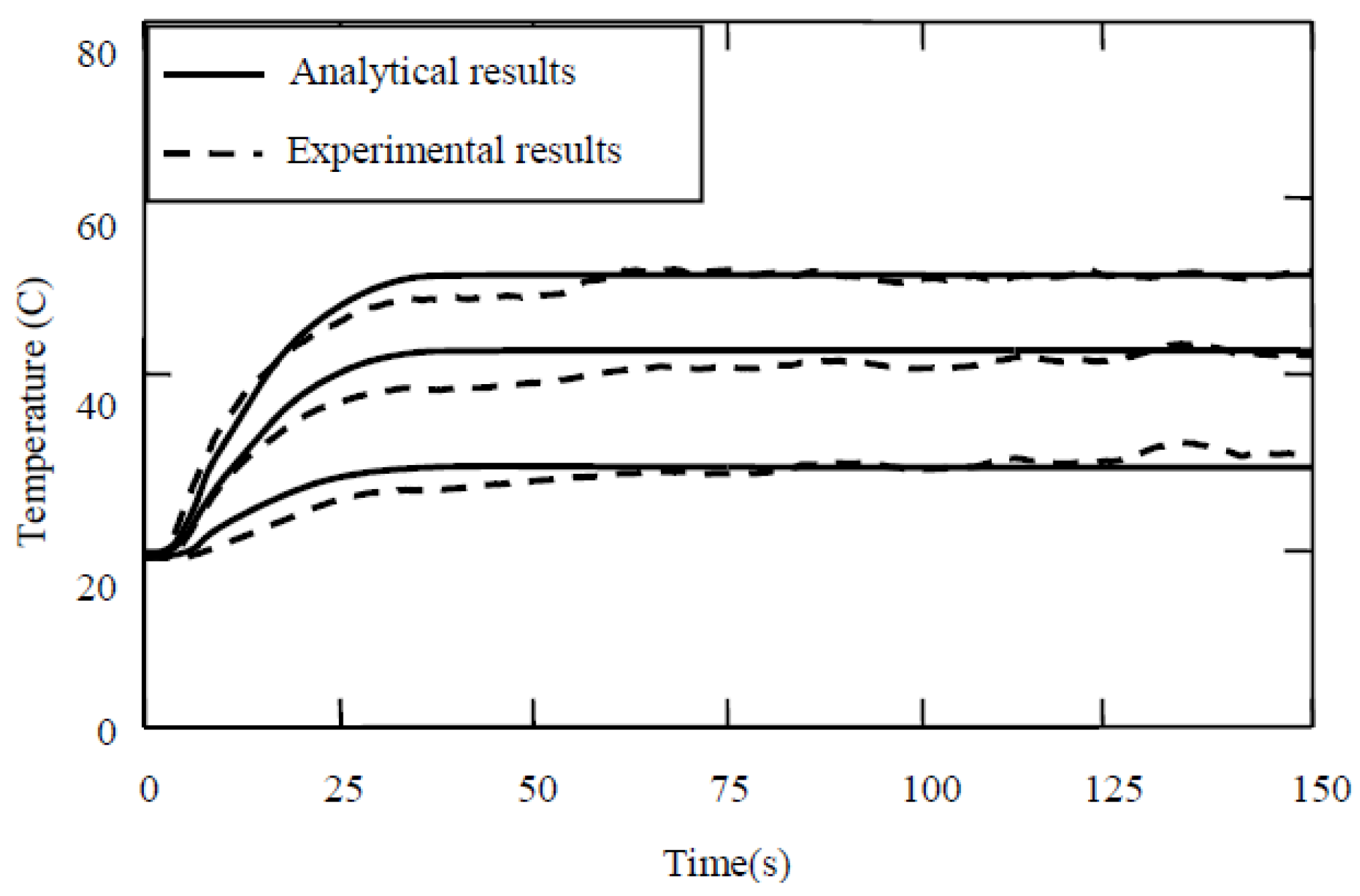
Results of the experimental with comparisons demonstrates that the measured temperature data are highly consistent with those of numerical simulations.
- (3)
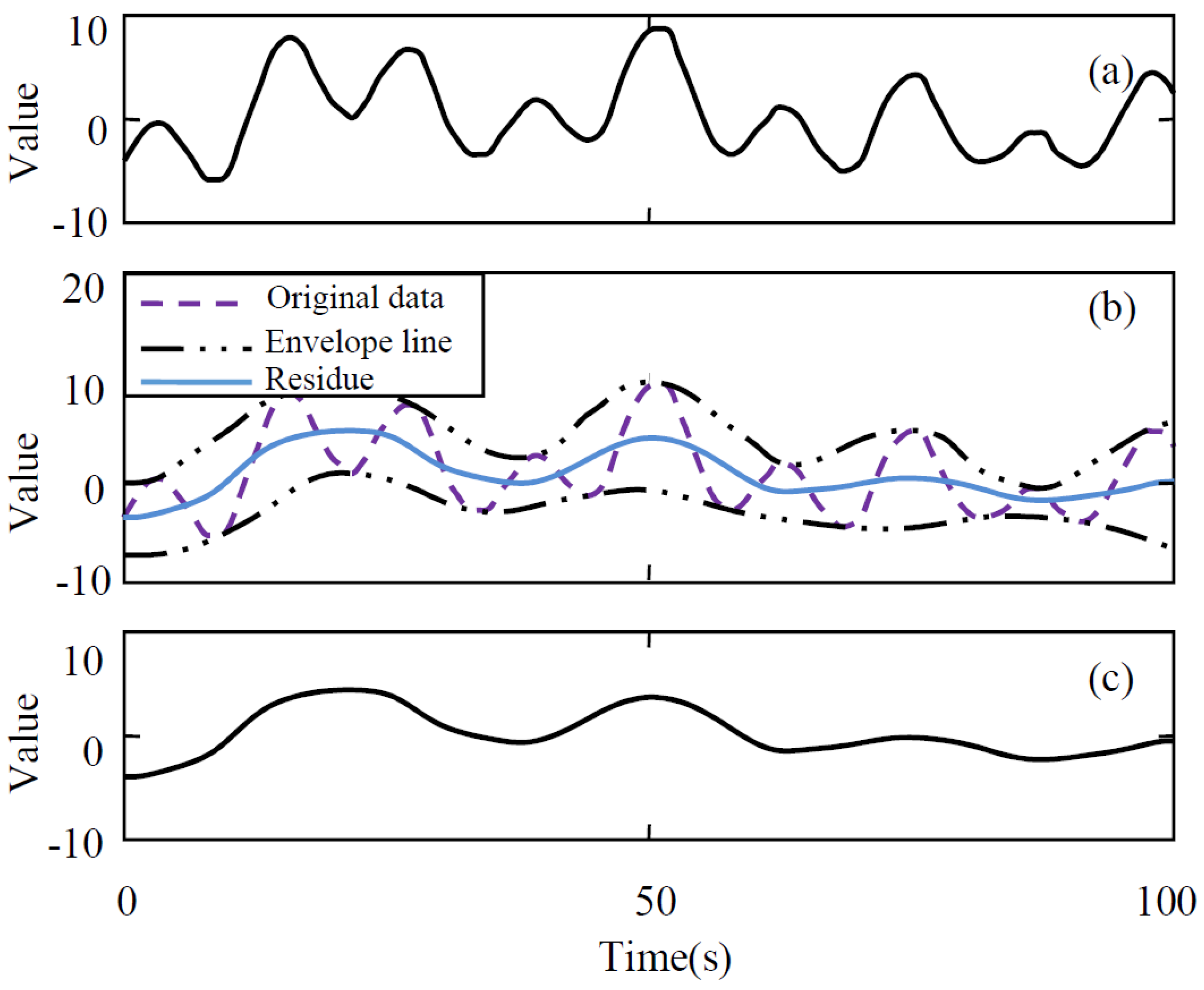
The new type of mean filter, proposed based on principles of EMD, is very convenient for application to the data processing and has a remarkable suppressing ability for the high-frequency components.
According to the presented results, the proposed tool design and cooling solution can be also utilized for the machining of other materials. In the future, it would be worthwhile to investigate fluid of higher heat transfer coefficients on the independent cooling structure. Some other non-contact temperature measure methods are also worthy of further exploration.


 ,
, 


