Reconstruction to Sensor Measurements Based on a Correlation Model of Monitoring Data

Abstract

A sensor failure will lead to sensor measurement distortion, and may reduce the reliability of the whole structure analysis. This paper studies the method of monitoring information reconstruction based on the correlation degree. For the faulty sensor, the correlation degree of the normal response of this sensor and the measurements of the other sensors is calculated, which is also called the correlation degree of reconstructed variables and response variables. By comparing the correlation degrees, the response variables, which are needed to establish the correlation model, are determined. The correlation model between the reconstructed variables and the response variables is established by the partial least square method. The value of the correlation degrees between the reconstructed variables and the response variables, the amount of the monitoring data which is used to determine the coefficients of the correlation model, and the number of the response variables are used to discuss the influence factors of the reconstruction error. The stress measurements of structural health monitoring system of Shenzhen Bay Stadium is taken as an example, and the effectiveness of the method is verified and the practicability of the method is illustrated.

1. Introduction

The sensors are the basic instruments of the structural health monitoring system, while the measurements of sensors are the necessary information for estimating the structural safety. However, the operation duration of a sensor is limited and the sensor measurements may be abnormal because of sensor failure or environmental influences [1]. The technique for reconstructing the sensor information should be developed as a result, which can ensure saving the complete monitoring information for structural safety estimation. The monitoring information is diverse in the different measured locations and the different types of structural responses, which are correlated with each other to some extent [2]. That is to say, it is necessary to reconstruct the information for the failure sensor using the effective correlation model between the failure sensor and the other normal sensors.

For the sensor information reconstruction, the researchers proposed several methods to solve the question. For the problem of data distortion in the structural health monitoring system of a bridge, Huang [3] analyzed the relationship of the monitoring data by using Granger causality testing [4] in which the sensor data with a closer relationship is selected to be the input vector for an extreme learning machine to recover the missing sensor signal data. However, the individual prediction value could be a large error, and the training results need to be further improved because the tendency of the predicted data is not consistent with the theory value. The radial basis function (RBF) neural network model is another method to recover the unreliable data, which is also easy to fall into a local optimum [5]. The Kalman filtering method was proposed to build the model between structural displacements and structural accelerations [6], in which the structural model parameters and external excitation should be known in advance. The method of data compression sampling is used for data recovery of wireless sensors, while the recovery data error would be larger for the accelerations when the sparse of the original data becomes worse [7]. Feng [8] proposed a data recovery method based on a least square support vector machine. A forecasting model based on the method is established, and signal recovery is accomplished by on-line learning diagnosis. However, this method mainly aims at the data reconstruction of the sensor within short duration, and the effect is not good for a high sampling rate and for long-term failure prediction.

This paper, thus, focuses on the structural responses and the correlation model between the reconstructed variable and the response variable is established, which can be used for reconstructing the sensor information. In this paper, the correlation degree and the partial least square method are applied to the data reconstruction of the fault sensors. As the strain sensors are placed on the roof steel structure of Shenzhen Bay Stadium, the strain measurements represent the distributed responses of the structure and have an inherent association, which is suitable to verify the effectiveness of the proposed method in the paper as well.

2. Correlation Model of Monitoring Data

2.1. Correlation Analysis of Monitoring Data

The monitoring structural responses from different locations and different types of sensors are in the correlated relationship. The Pearson correlation coefficient is an index to measure the linear correlation degree of structural responses.

The structural response matrix of m measuring points under the load in n time steps is denoted as X:

$$X=\left[\begin{array}{cccc}{x}_1& x_2& ...& x_m\end{array}\right]=\left[\begin{array}{cccc}{x}_{11}& x_{12}& \cdots & x_{1m}\\ x_{21}& x_{22}& \cdots & x_{2m}\\ ⋮& ⋮& ⋮& ⋮\\ x_{n1}& x_{n2}& \cdots & x_{nm}\end{array}\right]$$

(1)

$$x_i={\left[\begin{array}{cccc}{x}_{i1}& x_{i2}& \cdots & x_{in}\end{array}\right]}^T$$

(2)

In the Equations (1) and (2), $x_i$ represents the measurements of the measuring point i under the load of n time steps. When the fault sensor works in normal, the measurement of the measuring point where the fault sensor located is denoted as $y$. The Pearson product-moment correlation coefficient [9] of the measurement from the arbitrary measuring point and the measuring point where the faulty sensor located is denoted as ρ_i

$${\rho }_i=\frac{\mathrm{cov}(x_i,y)}{{\mathsf{\sigma }}_{x_i}{\mathsf{\sigma }}_y}=\frac{E(x_i-{\mathsf{\mu }}_{x_i})(y-{\mathsf{\mu }}_y)}{{\mathsf{\sigma }}_{x_i}{\mathsf{\sigma }}_y}$$

(3)

$${\mathsf{\sigma }}_{x_i}=\frac{1}{n-1}{{\displaystyle \sum _{k=1}^n\left(x_i(k)-{\mathsf{\mu }}_{x_i}\right)}}^2$$

(4)

$${\mathsf{\sigma }}_y=\frac{1}{n-1}{{\displaystyle \sum _{k=1}^n\left(y(k)-{\mathsf{\mu }}_y\right)}}^2$$

(5)

$$\mathrm{cov}(x_i,y)=\frac{1}{n-1}{\displaystyle \sum _{k=1}^n\left(x_i(k)-{\mathsf{\mu }}_{x_i}\right)}\left(y(k)-{\mathsf{\mu }}_y\right)$$

(6)

In Equation (3), ${\mathsf{\sigma }}_{x_i}$ and ${\mathsf{\sigma }}_y$ represent the response variance of the measurement point i and the fault sensor, respectively; $\mathrm{cov}(x_i,y)$ is covariance, $x_i(k)$ and $y(k)$ represent the measurement of point i and the fault sensor in the k^th time step, respectively; ${\mathsf{\mu }}_{x_i}$ and ${\mathsf{\mu }}_y$ are the mean value of the measurements $x_i$ and $y$, respectively.

2.2. Correlation Modeling Using Partial Least Squares and Multiple Regression

2.2.1. Reconstructed Variable and Response Variables

The correlation coefficients of the normal measurement of fault sensor and the measurements of the other sensors are calculated, which are also called the correlation coefficients of the reconstructed variable and response variables. The correlation matrix can be denoted as P:

$$P=\left[\begin{array}{cccc}{\rho }_1& {\rho }_2& \cdots & {\rho }_m\end{array}\right]$$

(7)

The correlation coefficients are sorted from larger value to small value based on their absolute values, while the updated correlation coefficient’s sorting matrix can be denoted as D_P:

$$\begin{array}{cccc}{D}_P=\{{(\rho )}_1& \cdots {(\rho )}_i& \cdots & {(\rho )}_m\end{array}\}$$

(8)

(ρ)_i represents the i^th correlation coefficient absolute value, while (ρ)₁ is the largest correlation coefficient absolute value and (ρ)_m is the smallest correlation coefficient absolute value, respectively. The corresponding measurement to (ρ)_i is denoted as (x)_i, while the updated structural response sorting matrix can be denoted as D_X:

$$\begin{array}{cccc}{D}_X=\{{(x)}_1& \cdots {(x)}_i& \cdots & {(x)}_m\end{array}\}$$

(9)

The faulty sensor information is considered as the reconstructed variable $Y_P$, and p measurements are selected as response variables X_P:

$$\begin{array}{cccc}{X}_P=\{{(x)}_1& {(x)}_2& \cdots & {(x)}_p\end{array}\}$$

(10)

$$Y_P=\left\{y\right\}$$

(11)

2.2.2. Establishment of Correlation Model Using the Partial Least Square Method

The reconstructed variables and response variables are standardized as:

$${(x)}_i^{*}=\frac{{(x)}_i-{\mathsf{\mu }}_{{(x)}_i}}{{\mathsf{\sigma }}_{{(x)}_i}}$$

(12)

$$y^{*}=\frac{y-{\mathsf{\mu }}_y}{{\mathsf{\sigma }}_y}$$

(13)

The response variables $X_P$ and the reconstructed variable $Y_P$ are standardized into $E_0$ and $F_0$, respectively:

$$\begin{array}{cccc}{E}_0=\{{(x)}_1^{*}& {(x)}_2^{*}& \cdots & {(x)}_p^{*}\end{array}\}$$

(14)

$$F_0=\left\{y^{*}\right\}$$

(15)

The main components set of $E_0$ and $F_0$ can be obtained by using principal component analysis, which are denoted as $T$ and $U$, respectively:

$$T=\left\{\begin{array}{cccccc}{t}_1& t_2& ...& t_h& ...& t_A\end{array}\right\}$$

(16)

$$U=\left\{\begin{array}{cccccc}{u}_1& u_2& ...& u_h& ...& u_A\end{array}\right\}$$

(17)

The regression equations regarding $E_0$ and $F_0$ using partial least squares [10] and first principal components are:

$$E_0=t_1{p}_1{}^T+E_1$$

(18)

$$F_0=t_1{r}_1{}^T+F_1$$

(19)

where the regression coefficient vector is:

$$p_1=\frac{E_0^T{t}_1}{{\Vert t_1\Vert }^2}$$

(20)

$$r_1=\frac{F_0^T{t}_1}{{\Vert t_1\Vert }^2}$$

(21)

The regression equations for the h^th principal component are:

$$E_{h-1}=t_h{p}_h{}^T+E_h$$

(22)

$$F_{h-1}=t_h{r}_h{}^T+F_h$$

(23)

where the regression coefficient vector is:

$$p_h=\frac{E_{h-1}^T{t}_h}{{\Vert t_h\Vert }^2}$$

(24)

$$r_h=\frac{F_{h-1}^T{t}_h}{{\Vert t_h\Vert }^2}$$

(25)

The relationship between the h^th principal component t_h and the h^th axis of $E_0$ is:

$$t_h=E_{h-1}{w}_h$$

(26)

where $w_h$ is the unit eigenvector corresponding to the maximum eigenvalue ${\mathsf{\theta }}_h{}^2$ of matrix $E_{h-1}{}^T{F}_{h-1}{F}_{h-1}{}^T{E}_{h-1}$.

According to the Equations (18), (19), (22), and (23), $E_0$ and $F_0$ can be expressed as:

$$E_0=t_1{p}_1{}^T+t_2{p}_2{}^T+\cdots +t_h{p}_h{}^T+E_h$$

(27)

$$F_0=t_1{r}_1{}^T+t_2{r}_2{}^T+\cdots +t_h{r}_h{}^T+F_h$$

(28)

Substituting Equation (26) into Equation (22) yields:

$$E_h=E_{h-1}(I-w_h{p}_h{}^T)$$

(29)

Substituting Equations (26) and (29) into Equation (27) yields:

$$E_h=E_0{\displaystyle \prod _{j=1}^h(I-w_j}{p}_j{}^T)$$

(30)

Substituting Equation (30) into Equation (26) yields:

$$t_h=E_{h-1}{w}_h=E_0{\displaystyle \prod _{j=1}^{h-1}(I-w_j}{p}_j{}^T)w_h=E_0{w}_h{}^{*}$$

(31)

$$w_h*={\displaystyle \prod _{j=1}^{h-1}(I-w_j}{p}_j{}^T)w_h$$

(32)

Substituting Equation (31) into Equation (28) yields:

$$F_0=E_0{w}_1{}^{*}{r}_1{}^T+\cdots +E_0{w}_h{}^{*}{r}_h{}^T+F_h$$

(33)

Assuming the number of the principal components is h when the principal components satisfy the cross-validation principle. Meanwhile, $F_h$ approaches 0, which can be ignored. Equation (33) is written as:

$$F_0=E_0(w_1{}^{*}{r}_1{}^T+\cdots +w_h{}^{*}{r}_h{}^T)$$

(34)

Substituting Equations (14) and (15) into Equation (34) yields:

$$y*=[{(x)}_1^{*}\dots {(x)}_i^{*}\dots {(x)}_p^{*}]\left[\begin{array}{c}{\displaystyle \sum _{j=1}^h{r}_j}{w}_{j1}{}^{*}\\ \dots \\ {\displaystyle \sum _{j=1}^h{r}_j}{w}_{ji}{}^{*}\\ \dots \\ {\displaystyle \sum _{j=1}^h{r}_j}{w}_{jp}{}^{*}\end{array}\right]$$

(35)

If:

$${\mathsf{\alpha }}_i{}^{*}={\displaystyle \sum _{j=1}^h{r}_j}{w}_{ji}{}^{*}$$

(36)

then:

$$y^{*}={\mathsf{\alpha }}_1{}^{*}{(x)}_1{}^{*}+\cdots +{\mathsf{\alpha }}_p{}^{*}{(x)}_p{}^{*}$$

(37)

Substituting Equations (12) and (13) into Equation (37), the correlation model between the reconstructed variable and the response variables is:

$$y(i)={\mathsf{\alpha }}_1{(x(i))}_1+\cdots +{\mathsf{\alpha }}_p{(x(i))}_p+{\mathsf{\alpha }}_0$$

(38)

2.2.3. The Reconstruction Error Evaluation Index

The average absolute error between the reconstructed value and actual value e_a is:

$$e_a=\frac{1}{n}{\displaystyle \sum _{i=k}^n\left|y(k)-y_0(k)\right|}$$

(39)

The average relative error between the reconstructed value and actual value e_b is:

$$e_b=\frac{1}{n}{\displaystyle \sum _{k=1}^n\left|\frac{y(k)-y_0(k)}{y_0(k)}\right|}\times 100\%$$

(40)

where $y(k)$ represents the reconstructed response of k^th time step of the supposed fault sensor, and $y_0(k)$ represents the actual response of k^th time step of the supposed fault sensor, respectively.

3. Reconstruction to Stress Measurements of Shenzhen Bay Stadium

3.1. Project Description

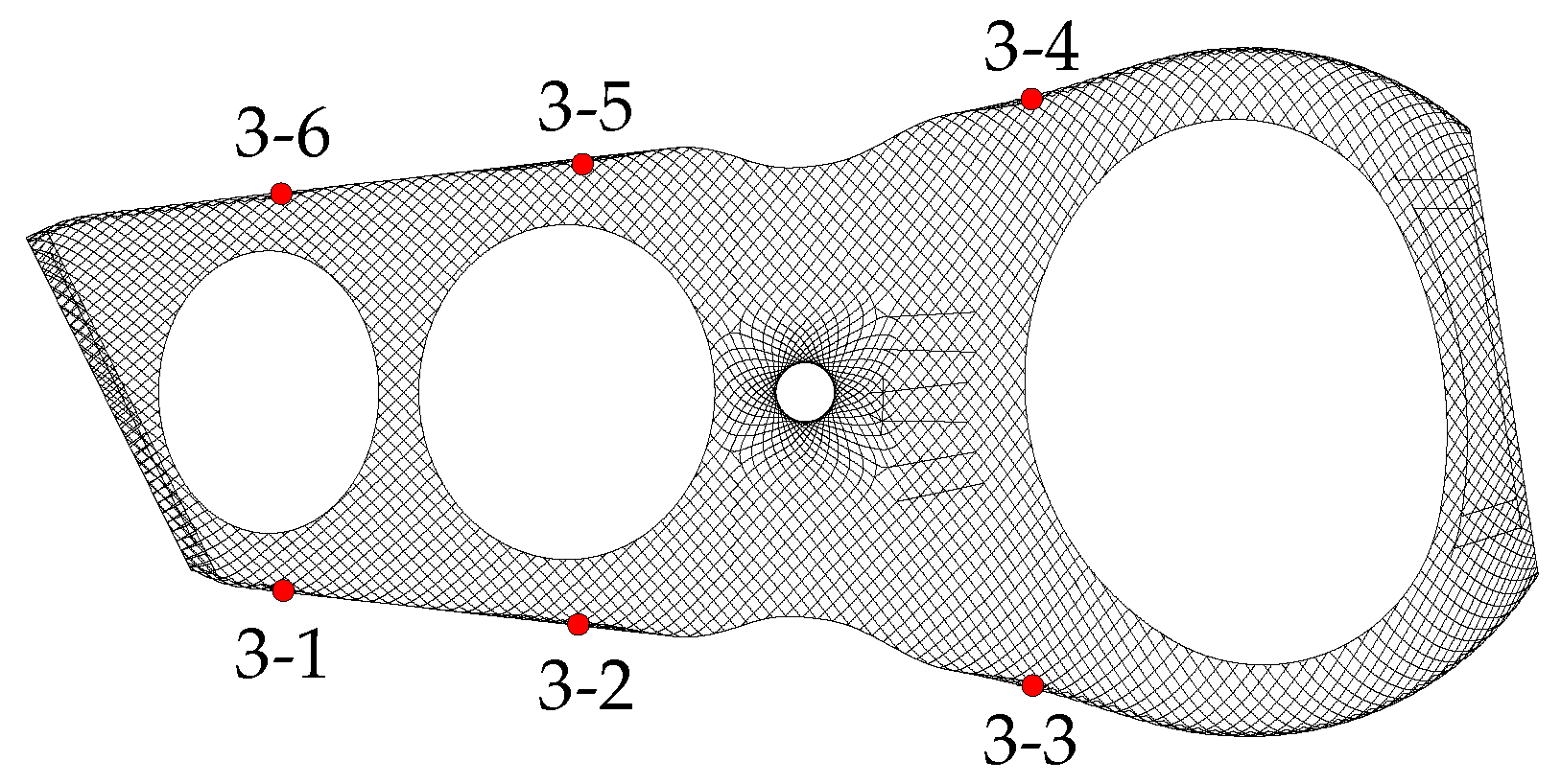
The structural health monitoring system of Shenzhen Bay Stadium began to be implemented in 2010, while the continuous monitoring of the steel roof in both the construction phase and service phase began to be carried out at the same time [11]. The stress measurements of the sensors located at the support members are chosen as the basic analysis data for example. 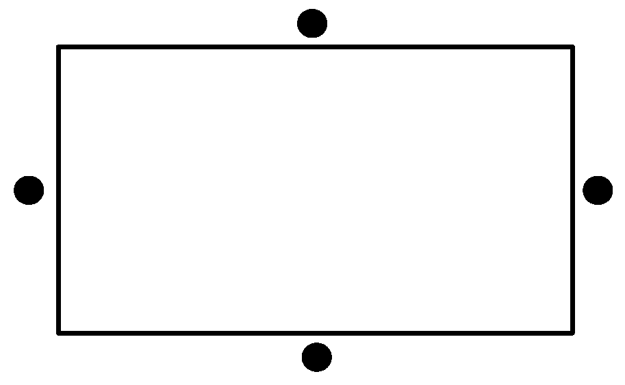The layout of sensors located at the support members are shown in Figure 1 and Figure 2. There are six supports, two rods of which are being monitored and four stress monitoring points are arranged on each rod; the sensor installation of support is shown in Figure 3. For example, the number of eight stress monitoring points at support 3-1 can be denoted as 3-1-1, 3-1-2, 3-1-3, 3-1-4, 3-1-5, 3-1-6, 3-1-7, and 3-1-8, respectively.

3.2. The Correlation Model of the Reconstructed Variable and the Response Variables

The sensor at location 3-1-4 is assumed to be failure on 16 May 2014. The stress monitoring information of this point is considered as the reconstructed variable. The measurements of the other locations are considered as the available response variables. The stress monitoring data from 7 May 2014 to 10 May 2014 are selected to calculate the correlation coefficients between measurements from location 3-1-4 and the other locations, which are shown in

Table 1. The correlation degree of stress monitoring data between stress sensor 3-1-4 and other stress sensors.

Ranking	Sensor Location	Correlation Coefficient	Ranking	Sensor Location	Correlation Coefficient
1	3-1-8	0.6831	18	3-1-2	0.2076
2	3-6-6	0.5437	19	3-6-1	0.1975
3	3-3-2	0.5194	20	3-5-1	0.1962
4	3-2-8	0.4656	21	3-1-3	0.1623
5	3-1-7	0.4212	22	3-2-7	0.1113
6	3-2-4	0.4121	23	3-6-8	0.0915
7	3-1-6	0.4006	24	3-3-7	0.0742
8	3-2-6	0.3735	25	3-2-2	0.0632
9	3-5-7	0.3688	26	3-3-1	0.0624
10	3-2-3	0.3677	27	3-3-3	0.0547
11	3-5-4	0.3608	28	3-2-5	0.0424
12	3-6-3	0.3512	29	3-5-2	0.0214
13	3-5-5	0.3425	30	3-5-8	0.0156
14	3-3-6	0.3289	31	3-5-3	0.0141
15	3-5-6	0.2745	32	3-6-4	0.0108
16	3-1-5	0.2608	33	3-2-1	0.0031
17	3-1-1	0.2487	-	-	-

.

In Equation (38), there is no exact number demanded of the response variables, which may depend on the detailed examples and the special value of the correlation coefficients. Generally speaking, the historical measurements can be used to identify the effectiveness when the different number of responses variables selected. If four response variables are chosen to build the correlation model, that is to say, p = 4, then:

$$\begin{array}{cccc}{D}_P=\{0.6831& -0.5437& -0.5194& 0.4656\end{array}\}$$

(41)

$$\begin{array}{ll}\hfill X_{P1}& =\left\{\begin{array}{cccc}{(x)}_1& {(x)}_2& {(x)}_3& {(x)}_4\end{array}\right\}\hfill \\ & =\left\{\begin{array}{cccc}{\mathsf{\sigma }}_{3-1-8}\left(t\right)& {\mathsf{\sigma }}_{3-6-6}(t)& {\mathsf{\sigma }}_{3-3-2}(t)& {\mathsf{\sigma }}_{3-2-8}(t)\end{array}\right\}\hfill \end{array}$$

(42)

$$Y_{P1}=\left\{y_1\right\}{=\{\mathsf{\sigma }}_{3-1-4}(t)\}$$

(43)

The correlation model of the reconstructed variable and the response variable is:

$$y_1(i)=1.01{(x(i))}_1+0.05{(x(i))}_2-0.09{(x(i))}_3+0.10{(x(i))}_4-20.73$$

(44)

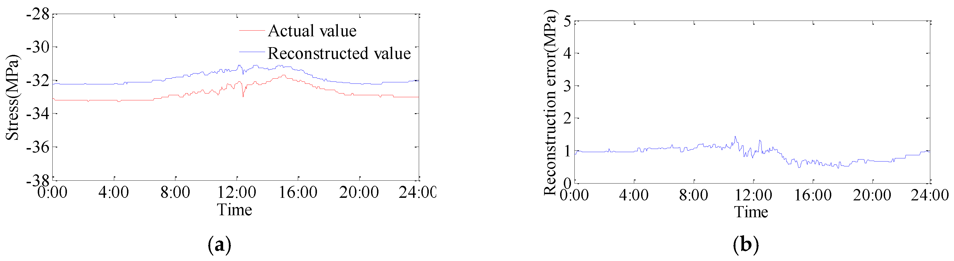
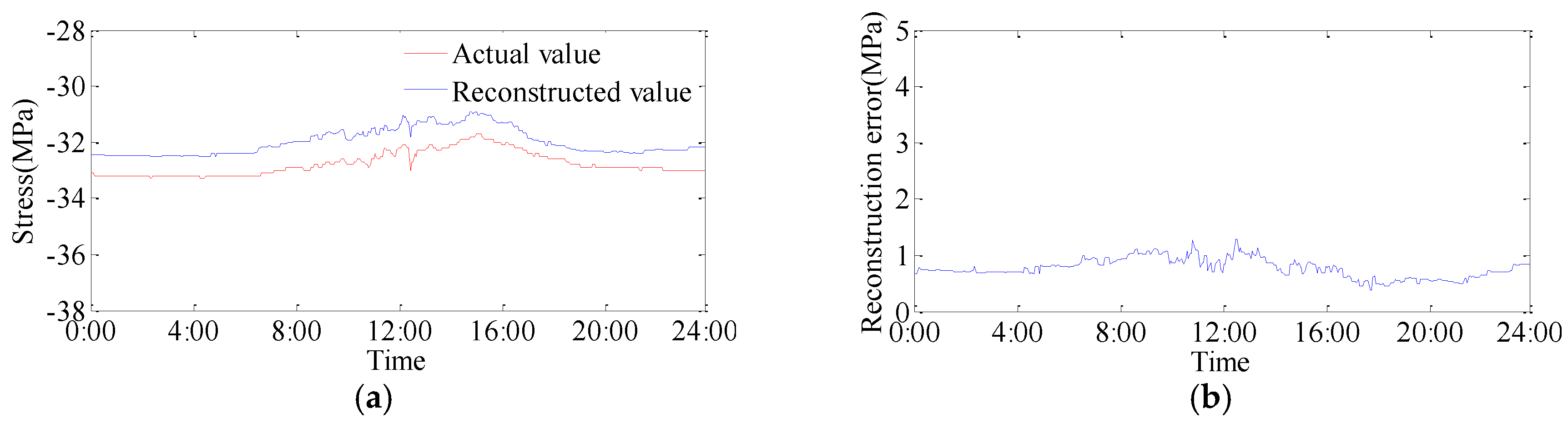
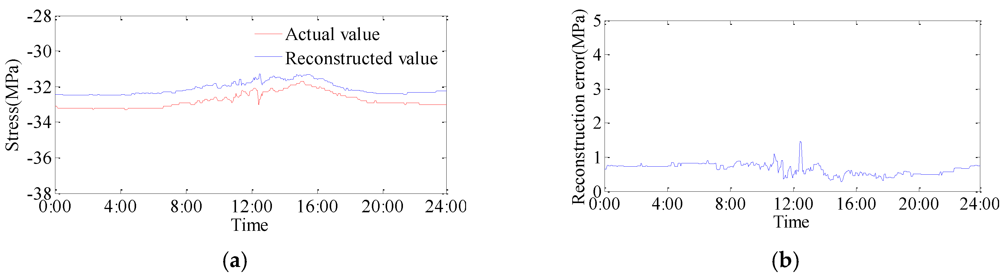
The stress monitoring data of the stress sensor 3-6-6, 3-3-2, 3-1-8, and 3-2-8 are used to reconstruct the stress measurements of the sensor located at point 3-1-4 on 16 May 2014. The contrast curves between reconstructed values and actual values are shown in Figure 4. The reconstructed values have the same trend as the actual values, and there are small differences between them. The average absolute error is 0.89 MPa and the relative error is 2.71%.

3.3. Influence of Correlation Degree on Reconstruction Error

In order to discuss the influences of the selection of response variables, two additional cases are discussed, which are:

$$\begin{array}{cc}\hfill X_{P2}& =\left\{\begin{array}{cccc}{(x)}_{13}& {(x)}_{14}& {(x)}_{15}& {(x)}_{16}\end{array}\right\}\hfill \\ & =\left\{\begin{array}{cccc}{\mathsf{\sigma }}_{3-5-5}(t)& {\mathsf{\sigma }}_{3-3-6}(t)& {\mathsf{\sigma }}_{3-5-6}(t)& {\mathsf{\sigma }}_{3-1-5}(t)\end{array}\right\}\hfill \end{array}$$

(45)

and:

$$\begin{array}{cc}\hfill X_{P3}& =\left\{\begin{array}{cccc}{(x)}_{30}& {(x)}_{31}& {(x)}_{32}& {(x)}_{33}\end{array}\right\}\hfill \\ & =\left\{\begin{array}{cccc}{\mathsf{\sigma }}_{3-5-8}(t)& {\mathsf{\sigma }}_{3-5-3}(t)& {\mathsf{\sigma }}_{3-6-4}(t)& {\mathsf{\sigma }}_{3-2-1}(t)\end{array}\right\}\hfill \end{array}$$

(46)

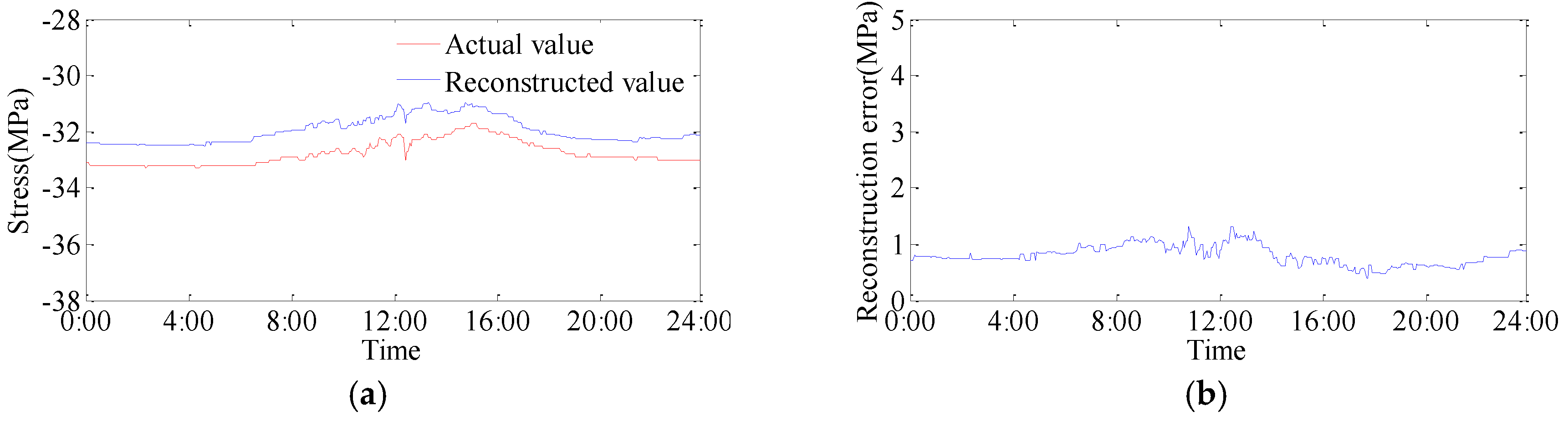
The correlation model using $X_{P2}$ is:

$$y_2(i)=0.02{(x(i))}_{13}+0.01{(x(i))}_{14}+0.39{(x(i))}_{15}+0.02{(x(i))}_{16}-23.85$$

(47)

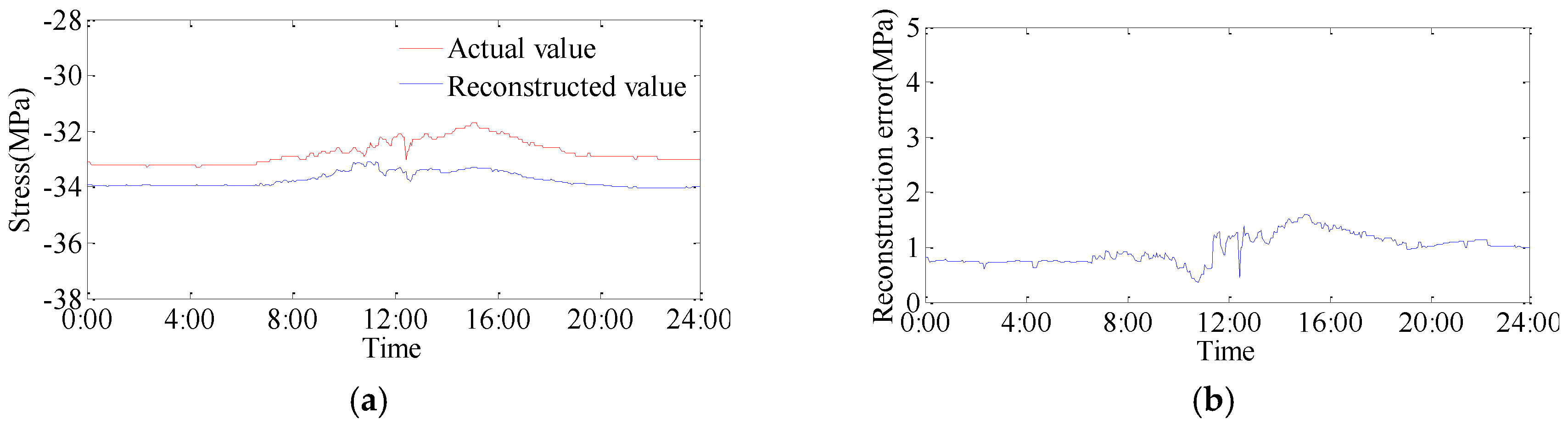
The contrast curves between reconstructed values and actual values are shown in Figure 5. The average absolute error is 0.97 MPa and the relative error is 2.97%.

The correlation model using $X_{P3}$ is:

$$y_3(i)=-0.01{(x(i))}_{30}+0.01{(x(i))}_{31}-0.01{(x(i))}_{32}-0.01{(x(i))}_{33}-32.03$$

(48)

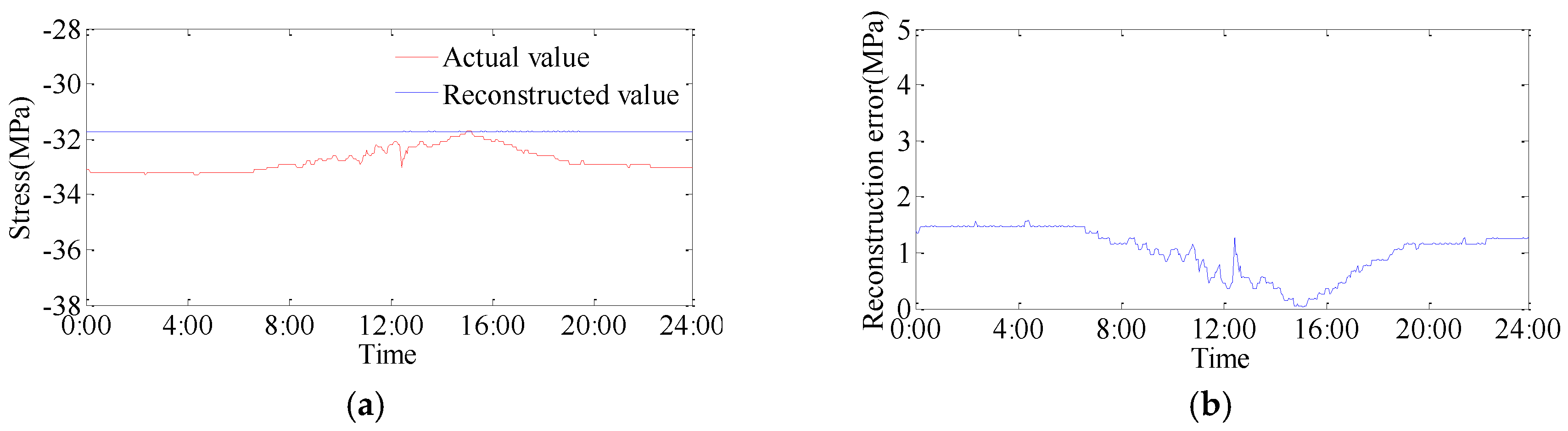
The contrast curves between reconstructed values and actual values are shown in Figure 6. The average absolute error is 1.03 MPa and the relative error is 3.13%.

The errors of the reconstructed information using different correlation coefficients of the response variables are summarized in

Table 2. The summarized errors using different response variables.

Response Variables	ea (MPa)	eb
$X_{P1}$	0.89	2.71%
$X_{P2}$	0.97	2.97%
$X_{P3}$	1.03	3.13%

.

It can be seen from Table 2 that the errors become larger when the coefficients of response variables become smaller, in which the average absolute error and relative error are minimum when X_P1 is chosen as the response variables. It indicated that the response variables with closer correlation to the reconstructed variable should be chosen, which is better for the reconstruction of the sensor measurements.

3.4. Influence of Monitoring Data Quantity on Reconstruction Error

In order to discuss the influences of the selection of response variables, two additional cases are discussed. The original stress monitoring data is collected from 7 May 2014 to 10 May 2014 to calculate the correlation coefficients between measurements from location 3-1-4 and the other locations. The stress monitoring data of two additional cases are from 7 May 2014 to 12 May 2014 and from 7 May 2014 to 14 May 2014, respectively.

The correlation model using stress monitoring data from 7 May 2014 to 12 May 2014 is:

$$y_4(i)=0.89{(x(i))}_1+0.09{(x(i))}_2-0.20{(x(i))}_3+0.04{(x(i))}_4-33.62$$

(49)

The contrast curves between reconstructed values and actual values are shown in Figure 7. The average absolute error is 0.65 MPa and the relative error is 1.99%.

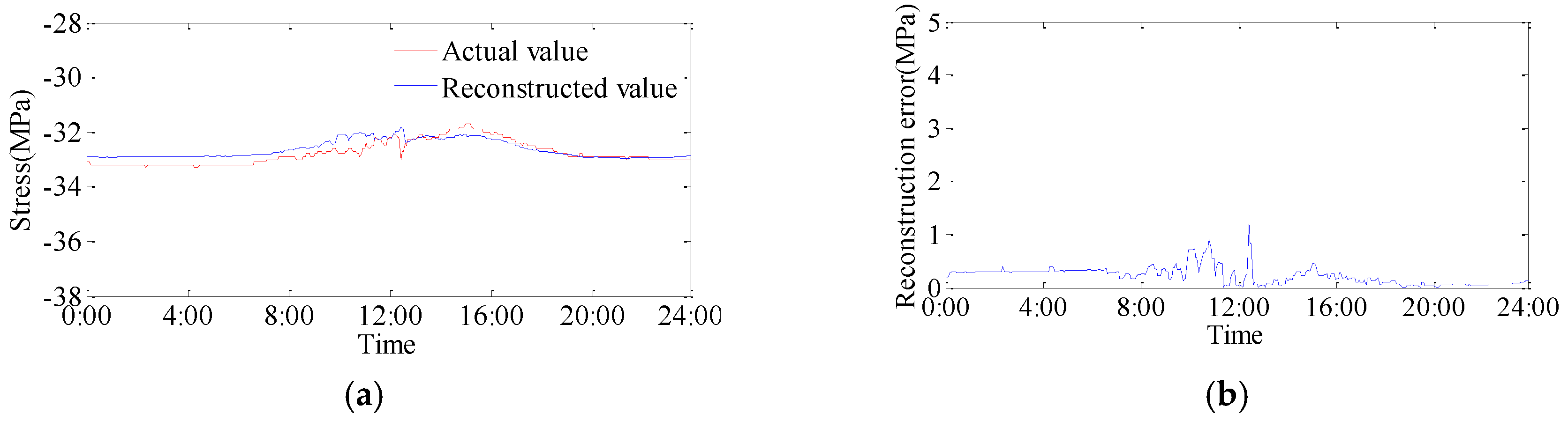
The correlation model using stress monitoring data from 7 May 2014 to 14 May 2014 is:

$$y_5(i)=0.35{(x(i))}_1-0.16{(x(i))}_2-0.11{(x(i))}_3+0.03{(x(i))}_4-39.45$$

(50)

The contrast curves between the reconstructed values and the actual values are shown in Figure 8. The average absolute error is 0.22 MPa and the relative error is 0.68%.

The errors of the reconstructed information using stress monitoring data from different time periods are summarized in

Table 3. The summarized errors using stress monitoring data from different time periods.

Data Acquisition Time	ea (MPa)	eb
2014.05.07~2014.05.10	0.89	2.71%
2014.05.07~2014.05.12	0.65	1.99%
2014.05.07~2014.05.14	0.22	0.68%

.

It can be seen from Table 3 that the errors become smaller when the quantity of stress monitoring data become larger, in which the average absolute error and relative error are a minimum when the stress monitoring data from 7 May 2014 to 12 May 2014 is chosen to build the correlation model. This indicated that the larger quantity of stress monitoring data should be used, which is better for reconstruction of sensor measurements. In theory, the number of measurements larger than the unknown coefficients is the basic requirement for regression function identification; in fact, there are noises and temperature effects included in the measurements, the measurements in at least one full day are better.

3.5. Influence of Response Variable Number on Reconstruction Error

In order to discuss the influences of the different number of response variables, three additional cases are discussed, which are:

$$\begin{array}{cccc}{X}_{P5}=\{{(x)}_1& {(x)}_2& {(x)}_3& \begin{array}{cc}{(x)}_4& {(x)}_5\end{array}\end{array}\}$$

(51)

$$\begin{array}{cccc}{X}_{P6}=\{{(x)}_1& {(x)}_2& {(x)}_3& \begin{array}{cc}{(x)}_4& \begin{array}{cc}{(x)}_5& {(x)}_6\end{array}\end{array}\end{array}\}$$

(52)

$$\begin{array}{cccc}{X}_{P7}=\{{(x)}_1& {(x)}_2& {(x)}_3& \begin{array}{cc}{(x)}_4& \begin{array}{cc}{(x)}_5& \begin{array}{cc}{(x)}_6& {(x)}_7\end{array}\end{array}\end{array}\end{array}\}$$

(53)

The correlation model using $X_{P5}$ is:

$$y_6(i)=1.33{(x(i))}_1+0.10{(x(i))}_2-0.03{(x(i))}_3-0.08{(x(i))}_4-0.20{(x(i))}_5-32.82$$

(54)

The contrast curves between reconstructed values and actual values are shown in Figure 9. The average absolute error is 0.80 MPa and the relative error is 2.45%.

The correlation model using $X_{P6}$ is:

$$y_7(i)=1.33{(x(i))}_1+0.11{(x(i))}_2-0.04{(x(i))}_3-0.11{(x(i))}_4-0.16{(x(i))}_5+0.08{(x(i))}_6-30.95$$

(55)

The contrast curves between reconstructed values and actual values are shown in Figure 10. The average absolute error is 0.80 MPa and the relative error is 2.44%.

The correlation model using $X_{P7}$ is

$$y_8=1.30{(x)}_1+0.09{(x)}_2-0.07{(x)}_3-0.08{(x)}_4-0.19{(x)}_5+0.12{(x)}_6+0.13{(x)}_7-26.93$$

(56)

The contrast curves between the reconstructed values and the actual values are shown in Figure 11. The average absolute error is 0.77 MPa and the relative error is 2.36%.

The errors of the reconstructed information using different number of the response variables are summarized in

Table 4. The summarized errors using different number of the response variables.

Response Variable	ea (MPa)	eb
$X_{P1}$	0.89	2.71%
$X_{P5}$	0.80	2.45%
$X_{P6}$	0.80	2.44%
$X_{P7}$	0.77	2.36%

.

It can be seen from Table 4 that the errors become smaller when the number of response variables become larger, in which the average absolute error and relative error are minimum when X_P7 is chosen as the response variables. However, there is only a slight difference between these discussed cases, and the number of the response variables with the same level of correlation coefficients influencing the errors of the reconstructed variables.

4. Conclusions

In this paper, a method of sensor information reconstruction based on the correlation degree is proposed. The monitoring information of a faulty sensor can be reconstructed by the correlation model and the measurements of other normal sensors. Based on the structural health monitoring system of Shenzhen Bay Stadium, the stress measurements of sensors located at support members are used to verify the proposed method. Furthermore, the influences for the errors of reconstructed monitoring information of a faulty sensor caused by three kinds of factors are discussed in the paper, which are the selection of response variables with different correlation, the quantity of the measurements from different time periods, and the number of response variables. The selection of response variables and the quantity of the measurements from different time periods are two main factors, which influence the reconstructed information errors for the faulty sensor directly. The number of the response variables influences the errors of reconstructed information a little if the selected response variables are in the same correlation level to reconstructed variable. Furthermore, the proposed method is verified its effectiveness to a real world project.

References

- Yeung, W.T.; Smith, J.W. Damage detection in bridges using neural networks for pattern recognition of vibration signatures. Eng. Struct. 2005, 27, 685–698. [Google Scholar] [CrossRef]
- Agrawal, R.; Imielinski, T.; Swami, A.N. Mining association rules between sets of items in large databases. In Proceedings of the 1993 ACM SIGMOD International Conference on Management of Data, 26–28 May 1993; ACM: Washington, DC, USA; pp. 207–216.
- Huang, Y.W.; Wu, D.G.; Li, J. Structural healthy monitoring data recovery based on extreme learning machine. Comput. Eng. 2011, 37, 241–243. (In Chinese) [Google Scholar]
- Hu, S.R.; Chen, W.M.; Cai, X.X.; Liang, Z.B.; Zhang, P. Research of deflection data compensation by applying artificial neural networks. In Proceedings of the 2nd International Conference on Structural Health Monitoring of Intelligent Infrastructure, Shenzhen, China, 16–18 November 2005; Taylor & Francis-Balkema: Leiden, The Netherlands; pp. 755–758.
- Huang, G.B.; Zhu, Q.Y.; Siew, C.K. Extreme learning machine: Theory and applications. Neurocomputing 2006, 70, 489–501. [Google Scholar] [CrossRef]
- Ma, T.W.; Bell, M.; Lu, W.; Xu, N.S. Recovering structural displacements and velocities from acceleration measurements. Smart. Struct. Syst. 2014, 14, 191–207. [Google Scholar] [CrossRef]
- Bao, Y.Q.; Li, H.; Sun, X.D.; Yu, Y.; Ou, J.P. Compressive sampling-based data loss recovery for wireless sensor networks used in civil structural health monitoring. Struct. Health Monit. 2013, 12, 78–95. [Google Scholar] [CrossRef]
- Feng, Z.G.; Shida, K.; Wang, Q. Sensor fault detection and data recovery based on LS-SVM predictor. Chin. J. Sci. Instrum. 2007, 28, 193–197. [Google Scholar]
- Pearson, K. Notes on regression and inheritance in the case of two parents. Proc. R. Soc. Lond. 1895, 58, 240–242. [Google Scholar] [CrossRef]
- Tenenhaus, M.; Esposito Vinzi, V.; Chatelinc, Y.-M.; Lauro, C. PLS path modeling. Comput. Stat. Data Anal. 2005, 48, 159–205. [Google Scholar] [CrossRef]
- Teng, J.; Lu, W.; Cui, Y.; Zhang, R.G. Temperature and displacement monitoring to steel roof construction of Shenzhen Bay Stadium. Int. J. Struct. Stab. Dyn. 2016, 16, 1640020. [Google Scholar] [CrossRef]
© 2017 by the authors. Licensee MDPI, Basel, Switzerland. This article is an open access article distributed under the terms and conditions of the Creative Commons Attribution (CC BY) license ( http://creativecommons.org/licenses/by/4.0/).