Abstract
Traffic noise is one of the main pollutants in urban and suburban areas. European authorities have driven several initiatives to study, prevent and reduce the effects of exposure of population to traffic. Recent technological advances have allowed the dynamic computation of noise levels by means of Wireless Acoustic Sensor Networks (WASN) such as that developed within the European LIFE DYNAMAP project. Those WASN should be capable of detecting and discarding non-desired sound sources from road traffic noise, denoted as anomalous noise events (ANE), in order to generate reliable noise level maps. Due to the local, occasional and diverse nature of ANE, some works have opted to artificially build ANE databases at the cost of misrepresentation. This work presents the production and analysis of a real-life environmental audio database in two urban and suburban areas specifically conceived for anomalous noise events’ collection. A total of 9 h 8 min of labelled audio data is obtained differentiating among road traffic noise, background city noise and ANE. After delimiting their boundaries manually, the acoustic salience of the ANE samples is automatically computed as a contextual signal-to-noise ratio (SNR). The analysis of the real-life environmental database shows high diversity of ANEs in terms of occurrences, durations and SNRs, as well as confirming both the expected differences between the urban and suburban soundscapes in terms of occurrences and SNRs, and the rare nature of ANE.
Keywords:
environmental sounds; dynamic noise maps; wireless acoustic sensor network; anomalous noise events; road traffic noise; recording campaign; audio database; acoustic salience; urban and suburban soundscapes PACS:
43.50.Rq; 43.60.Cg; 43.60.Bf
1. Introduction
Traffic noise is one of the main pollutants in urban and suburban areas that affects the quality of life of their citizens. As cities grow in size and population, the consequent increase in traffic is making this problem even more present and bothersome. In order to address this issue, European authorities have driven several initiatives to study, prevent and reduce the effects of exposure of population to traffic noise. Among them, the European Noise Directive (END) [1] is focused on the creation of noise level maps in order to inform citizens of their exposure to noise, besides drawing up appropriate action plans to reduce its negative impact. In general terms, these maps represent the equivalent noise level () and are updated every five years [1]. This is costly and time-consuming process that is undertaken by local and regional governments, and the resulting action plans can only be implemented and evaluated every five years.
These noise maps have been historically collected and generated by means of costly expert measurements using certified devices, based on short term periods that try to be as much representative as possible. However, this classic approach has recently undergone a dramatic change of paradigm thanks to the emergence of the so-called Wireless Acoustic Sensor Networks (WASNs) [2]. The WASN have been developed under the paradigms of both the Smart City and the Internet-of-Things.
In literature, we can find different WASN designed and deployed for several outdoor applications, some of which focus on security and surveillance purposes through the identification and localization of specific sounds related to hazardous situations. For instance, in [3], an ad-hoc WASN was designed to detect and locate shots for sniper detection. More recently, in [4] a WASN based on the FIWARE platform was deployed to locate and identify a broader type of sound sources such as people screaming or talking loudly, shot guns, horns, road accidents, etc. by including ambisonic microphones in the network. Finally, although no specific WASN is explicitly described, the proposal described in [5] is focused on the detection of road traffic accidents through the acoustic identification of tire skidding and car crashes.
Moreover, WASNs have also been deployed for city noise management, which involves noise mapping, action plans development, policing and improving public awareness, among others [6]. For instance, the SENSEable project [7] proposed a WASN to collect information about the acoustic environment of the city of Pisa (Italy) using low-cost acoustic sensors to study the relationship between public health, mobility and pollution through the analysis of citizens’ behaviour. Projects which have adopted a quite similar approach include the IDEA project in Belgium [8], the RUMEUR network in France [9] with a specific focus on aircraft noise, the ‘Barcelona noise monitoring network’ that is integrated in the Sentilo city management platform in Spain [10], or the DYNAMAP project, which is aimed at developing a dynamic noise mapping system able to detect and represent in real time the acoustic impact of road infrastructures in the cities of Rome and Milan (Italy) [11].
Nevertheless, the WASN paradigm poses several challenges, ranging from those derived from the design and development of the wireless sensor network itself [12,13], e.g., energy harvesting and low-cost hardware development and maintenance, to some specific challenges derived from the automation of the data collection and subsequent signal processing (see [2,14] and references therein). For instance, if the WASN is explicitly designed to measure road traffic noise levels, any acoustic event produced by any other noise source that could alter the measure (e.g., an air-craft flying over, nearby railways, road works, bells, crickets, etc.) should be detected and removed from the map computation to provide a reliable picture of the road noise level.
The detection of sound events is typically based on the segmentation of the input acoustic data into audio chunks that represent a single occurrence of a predefined acoustic class, separating them from other overlapping events if necessary [15], a task that is also denoted in the literature as polyphonic sound event detection, e.g., see [16,17]. The acoustic event detection and classification is closely related to the so-called computational auditory scene analysis (CASA) paradigm [18], which is devoted to acoustic scene classification and detection of sound events within an acoustic scene or soundscape [15]. These typically take advantage of being trained on specifically designed environmental databases containing the target finite set of acoustic classes (e.g., see [15,19,20]).
Therefore, it is necessary to design and develop representative audio databases containing this kind of non-desired sounds—hereafter denoted as anomalous noise events (ANE) [5,21]—to allow the signal processing block to automatically detect and discard them when captured by the WASN. However, the highly local, occasional, diverse and unpredictable nature of the ANE concept [21,22], together with the naturally unbalanced distribution of acoustic events in real-life environments [20,23] makes it difficult to build acoustic databases which are representative enough. This is of paramount importance to allow the WASN becoming reliable in front of ANEs, which should take into account the acoustic salience [24,25,26] of the anomalous noise event with respect to the background noise (i.e., a salient ANE should be detected and removed from the road traffic noise computation to avoid biasing the noise map generation). To tackle this problem, several works have tried to build these databases by artificially mixing background noise with ANEs and considering different event-to-noise ratio (hereafter, Signal-to-Noise ratio or SNR) distributions, by mixing real background recordings with event excerpts from online digital repositories [21,27] or from isolated individual recording of actual sound sources [19,22]. Although this approach can help to improve the training process [22], it can also yield results that may not represent what is actually found in real-life environments due to acoustic data misrepresentation [28].
This article describes the design, recording campaign and analysis of a real-life environmental audio database of anomalous noise events gathered in the two pilot areas of the DYNAMAP project (http://www.life-dynamap.eu) [11]: an urban area within Milan’s district 9, and a suburban area along the Rome A90 highway. After manually labelling the collected samples of road traffic noise, background noise and anomalous noise events (subsequently divided into 19 subcategories), the description of the ANE is enriched through the automatic computation of their acoustic salience—defined as the contextual SNR of the event with respect to the traffic or background noise. The paper is completed with a comprehensive discussion on the obtained results that tries to shed light on several key aspects that should be taken into consideration when developing ANE databases for machine hearing approaches in real-life environments, and their implication for the modelling and automatic anomalous noise event recognition, whose development is out of the scope of this work. To our knowledge, no explicit studies have been previously conducted to consider the complexity of real-life soundscapes to provide the deployed WASN with the capability to discard ANEs from traffic noise map computation.
This paper is structured as follows. The work related to the most relevant previous attempts to generate environmental audio databases is explained in Section 2. Section 3 describes the generation and labelling of the real-life environmental audio database in the urban and suburban scenarios of the two pilot areas of the DYNAMAP project, and provides detailed description of the recording campaign, the annotation of ANE and the automatic process used to annotate the ANE contextual SNRs. Section 4 analyses the ANE of both urban and suburban audio data in terms of occurrences, durations and SNRs. Next, Section 5 discusses in detail the results obtained from the database analyses, and the paper finishes with the main conclusions and future work in Section 6.
2. Related Work
In this section, firstly, the most relevant recent attempts to collect environmental audio data for aesthetic, heritage and scientific purposes are described. Next, several works related to the labelling with special emphasis on the determination of the salience of the audio events are detailed. A range of approaches are described from those designed to identify salient events regardless of their nature, to those that opt for their artificial generation.
2.1. Environmental Audio Databases
During the last decade, diverse online digital repositories containing environmental audio recordings have been developed. Among them, several online platforms have been designed as a query-based content supplier service where the user is also allowed to upload new audio clips (e.g., Freesound (https://www.freesound.org), Soundcloud (https://soundcloud.com), AudioHero (http://www.audiohero.com), StockMusic (http://stockmusic.com/), etc.). Other online repositories are devoted to sharing audio information from ecological and/or cultural perspectives with the aim of providing a testimony of environmental sounds of nature and cultures (e.g., EarthEar (http://www.earthear.com) or AcousticEcology (http://www.acousticecology.org)). Similarly, some sites provide long recordings of environmental soundscapes (e.g., Listen to Africa (http://www.listentoafrica.com/audio) or Open Sound New Orleans (http://www.opensoundneworleans.com)), while other sites have been designed as digital libraries of sound events (e.g., Macaulay Library (http://macaulaylibrary.org) for animal sounds or Xeno Canto (http://www.xeno-canto.org), specifically devoted to bird songs). However, since they are either oriented to provide audio clips for aesthetic purposes (e.g., for a soundtrack of a film production) or intangible culture heritage (e.g, saving a particular soundscape), almost no attention is given to validating the quality of the uploaded audio files and their corresponding meta-data (e.g., audio format, sound sources, recording equipment, etc.), which are key aspects in ensuring data reliability for possible derived scientific studies.
During the same period, the environmental audio research community has built some standardized databases for comparative purposes. Some examples of this attempt are the following: Freefield1010 [29], which integrated samples from the FreeSound database, MIVIA road Audio Events Dataset (http://mivia.unisa.it/datasets/audio-analysis/mivia-road-audio-events-data-set) [19], containing sound events, namely tire skidding and car crashes, for road surveillance applications, and the “ESC: Dataset for Environmental Sound Classification” [30], including 250,000 recordings extracted from FreeSound (tagged as “field recording”). Last but not least, in [16] a 19h audio database covering 10 audio contexts of indoor and outdoor environments (including transport and leisure scenarios) was described and evaluated for context-dependent sound event detection (The reader is referred to http://www.cs.tut.fi/~heittolt/datasets for a complete collection of this kind of databases).
Going a step further, specific databases have also been made available to the research community through specific competitions or challenges in recent years, following previous similar attempts such as the CLEAR 2007 evaluation for indoor environments [31]. Giannoulis et al. [15] describe the database provided for the Detection and Classification of Acoustic Scenes and Events (DCASE) 2013 challenge, where live and synthetic recordings were used to assess automatic detection and classification of audio events occurring within a scene. The reader is referred to [32] for the detailed analysis and discussion on the competition results. More recently, Mesaros et al. [20] have created the TUT Acoustic Scenes 2016 database, used in the DCASE 2016 challenge (http://www.cs.tut.fi/sgn/arg/dcase2016) to assess the performance of several automatic event or acoustic scenes detection systems in 15 different acoustic environments. The TUT sound outdoor events are oriented to safety and surveillance and human activity monitoring in residential areas and consider events bird singing, people speaking or walking, wind blowing, or car pass-bys as detectable. Although they provide real-life audio data, the goal of the described task (a standard n-class classification) differs from the problem at hand significantly (a binary classification task between traffic and non-traffic noise). In this sense, we want to underline the fact that the authors state that they only provide the eleven acoustic classes identified in the residential area as ground truth, disregarding the rest of acoustic events present in the recorded audio. However, those events should be also detected and discarded from the traffic noise map computation for the goal described in this work.
2.2. Salience of Environmental Acoustic Events
After collecting representative acoustic data for building environmental databases, a labelling process should be conducted, which becomes particularly complex when dealing with real-life recordings. This is of special importance when it comes to delimiting the boundaries of each sound event, i.e., determining the start and end points of each sound event in the mixed audio data [15,17] and the event/background ratio salience [24,25,26]. In the context of environmental sounds, it is important to highlight that acoustic events are usually disconnected from one another, which contrasts with speech or music where a strongly interconnected temporal structure of basic units is present (phonemes and notes, respectively) [33].
As far as the study of environmental acoustic events salience is concerned, diverse approaches depending on the application and the signal of interest can be found in the literature based on auditory attention (see [26] and references therein). These works are focused on determining perceptually important audio events according to human auditory response [24,25]. In [24], a model based on salience maps was designed to simulate the capability of human beings to switch their attention between different auditory stimuli over time, being evaluated on different types of transportation noise. In [25] an approach based on the computation of audio streams salience is applied to the audio summarization of movie segments, with environmental sounds such as wind or waves among the considered categories. In [26] an acoustic salience model designed to detect “unexpected” acoustic events is proposed and applied to control the overt attention of humanoid robots evaluated on the CLEAR 2007 database [31]. However, these salience-based approaches are designed to identify the salient event time boundaries (without regard to their origin) instead of measuring its relative energy difference with respect to background noise. To this aim, Salamon et al. [34] included a perceptually-based binary salience descriptor in their database, indicating whether that audio event was perceived to be in the foreground or background of the recording. The database was then used to evaluate a sound event classifier, which obtained better accuracies with foreground sound events than those perceived in the background. Hence, labelling the acoustic salience of audio events could permit more detailed sensitivity analyses of machine hearing approaches [33].
Alternatively, other research works opt for artificially mixing specific sound events with a certain background noise, e.g., see [19,21,32]. This way, on the one hand, there is an explicit control of the degree of salience of the audio events that should be detected, and on the other hand, it deals with one of the key problems of gathering such kind of data in real-life scenarios: data scarcity of specific audio events [22]. In [32], the authors proposed two parallel approaches to control the audio event density experimentally by conducting: (i) live recordings of scripted monophonic event sequences in controlled environments; and (ii) live recordings of individual events artificially combined with ambient background recordings into synthetic mixtures with parametrically controlled polyphony. For the latter, three SNR levels are considered: dB, 0 dB, and dB. In [22] an environmental database was recorded in real conditions containing major audio events such as: cicadas, outside air conditioner, road traffic noise, and neighbourhood noise. The authors extended that database with artificial mixtures of actual recordings of the events of interest in order to increase the sound sources diversity during the training stage of the proposed classifier. The inclusion of unseen mixtures within the training database was provided through varying the SNR level of three isolated sound sources in the mix, specifically: dB for cicadas, dB for outside air conditioner, and dB for ambulances. The results show that the classifier improves its overall accuracy in two of the three categories. However, these mixtures were generated without taking into account the real contribution of each sound source in the given acoustic environment. In [19] several typical sound events related to surveillance applications (e.g., scream, glass breaking and gunshot) were artificially mixed with other environmental sounds from indoor and outdoor environments with six different SNRs (from to dB at 5 dB step sweep) in order to simulate the occurrence of this kind of event in real and complex environments.
In [21], a mixture of sound sources considering road traffic noise plus other type of sound events was also generated using two different SNRs ( dB and dB) in order to assess the performance of an anomalous noise event detection algorithm (ANED). In this case, the ANEs were obtained from FreeSound while road traffic noise was recorded in a city ring road in real-life conditions. The experiments analysed different configurations of the ANED algorithm and showed quite good results when discriminating road traffic noise from those significantly salient ANEs. Finally, in [27] a small environmental audio database containing sound mixtures simulated with SimScene software [35] is described. The main argumentation of working with simulated sound mixtures is having a controlled experimental environment where the road traffic level is known beforehand. Unfortunately, there is no information available in this work about the SNR values considered to build the 20 scenes mixing background noise and car, bird and car horn samples.
Logically, the main drawback of these approaches is that the synthetic mixtures need not strictly follow real-life patterns. In the best case scenario, they could represent a subsampling of the actual picture of what is generally observed in average for the given acoustic environment. However, in the worst case, the significant difference with real-life conditions may lead to erroneous conclusions (e.g., see [28]).
3. Environmental Noise Database
In this section, the environmental audio database recorded and built in real-life conditions for the DYNAMAP project is detailed. Section 3.1 describes the urban and suburban pilot areas on-site inspection and recording campaign conducted to collect both road traffic noise and anomalous noise events samples. The subsequent audio database process generation, including the labelling and acoustic salience (computed as SNR) computation is described in Section 3.2.
3.1. Urban and Suburban Pilot Areas On-Site Inspections and Recording Campaign
The main goal of the recording campaign was to collect widely diverse samples of road traffic noise and anomalous noise events in order to provide a general picture of the real-life scenarios the dynamic noise mapping system will be working on. To that effect, several recordings were conducted between the 18 and 21 May 2015 in specific locations of the two pilot areas of the DYNAMAP project, covering both urban (Milan) and suburban (Rome) scenarios. These locations were selected according to representative traffic conditions and acoustic characteristics of the pilot areas (see [36,37] for further details).
The WASN of the DYNAMAP project is based on low-cost acoustic sensors from Bluewave [38]. According to the project requirements, the recordings were conducted using two measuring devices simultaneously: the low-cost sensor connected to a ZOOM H4n digital recorder (see Figure 1b), and a Bruel & Kjaer 2250 sonometer (see Figure 1a), being the latter used as a certified reference according to the project requirements. However, only the audio data obtained from the low-cost sensor is used for the subsequent analyses. The recording setup was the following:
- Situation of both measuring devices: 50 cm distance between them.
- Sampling: 48 kHz sampling rate with 24 bits/sample.
- Sensitivity verification using a 94 dBSPL, 1 kHz calibration tone.
- Clapping: in order to align the audio recordings from both measuring devices, a sequence of 5 s. of clapping was performed between both sensors with a separation that assured a very good signal to noise ratio despite the environmental noise.
- Gain adjustment: the input gain of each recorder was selected to guarantee enough room for in-site audio dynamics (no saturation).
- Installation: both recording systems were installed on a tripod and included a windscreen to protect the sensor from wind.
- Orientation: the final orientation of the DYNAMAP low-cost sensors with respect to the traffic flow is still undefined. For this reason, recordings were made with three orientations: putting the sensor in the direction of the traffic –forward orientation–, in the opposite direction –backward–, or orthogonal to the vehicles flow. Moreover, three elevation angles of the sensors positions were also employed: 0, 45 and −45.

Figure 1.
Recording equipment.
Between 18 and 19 May 2015 , the recordings were conducted in six sites along the A90 highway in Rome to collect suburban audio samples. They constituted a representative subset of the 17 sites in this pilot area according to the following four classes [36]: single road, additional crossing or parallel roads, railway lines running parallel or crossing the A90 motorway, and a complex scenario including multiple connections. In particular, the recording equipment was installed in six highway portals owned by the DYNAMAP partner ANAS S.p.A. (see Figure 2), a government-owned company under the control of the Ministry of Infrastructure and Transport in Italy. During these recordings, the weather conditions were dry and sunny, and with an average temperature of 19 C.
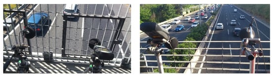
Figure 2.
Examples of the recording setup installed in the suburban scenario (Rome).
From 20 to the 21 May 2015, the recording campaign was moved to district 9 pilot area in Milan to collect urban road traffic noise samples in twelve locations at different times of day and night following [37] (see Figure 3 for examples of recording setup). More precisely, the recordings were conducted on the following locations:
- Near a hospital, including tramways and low traffic.
- One-way road with very-low traffic.
- Highly dense but slow traffic, with tramways, stone road surface, traffic lights and retentions.
- Railways, very-low traffic.
- Tram and railways, fast fluid traffic flow (multi-lane).
- City center, shopping road, crossroad with traffic lights. Wet road surface.
- Very low fluid traffic two-way road at night (multi-lane).
- Two-way road with fluid traffic near university (multi-lane).
- The same location as number 8 but with wet road surface.
- Narrow two-way road with fluid traffic in a residential area.
- Narrow two-way road with very-low-density traffic near a school.
- Low traffic, narrow one-way street near the city council.
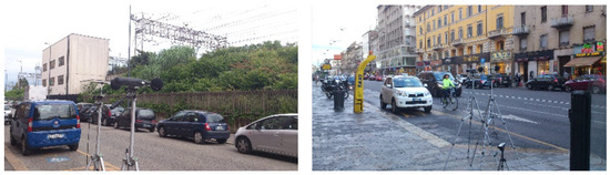
Figure 3.
Examples of the recording setup installed in the urban scenario (Milan).
During the Milan recordings the weather was quite sunny, except on the second day when there were thunderstorms during one of the recordings, and it was possible to record the noise of the thunder as well as road traffic noise with wet road surface.
As a result of the four-day recording campaign between the suburban (Rome) and urban (Milan) scenarios, a total of 9 h and 8 min of audio were collected and prepared for the subsequent labelling and post-processing phase, which is described in Section 3.2. For more details about the recording campaign, the reader is referred to [39].
3.2. Real-Life Urban and Suburban Environmental Audio Database Generation
After finishing the recording campaign, a post-processing phase was conducted in order to normalize and label all the recorded audio files and export them into analyzable audio clips. To that effect, we used the Audacity freeware software, generating a total of eighteen audio projects, one for each session during the recording campaign. Six projects were related to the suburban recordings, and twelve to the urban recordings, and their amplitude was normalized by using the calibration tone. Finally, each audio event was manually detected and labelled (including start and end points) by an expert annotator to guarantee the reliability of the annotation. The expert annotator was asked to annotate only those ANEs perceptually distinguishable from the background road traffic noise or from other acoustic events simultaneously occurring in the acoustic mixture.
Specifically, and after an initial listening revision, the expert was asked to distinguish between three major categories: road traffic noise (RTN, assigned to all audio regions containing road transit), background noise (BCK, reserved to those recordings where it was difficult to identify the noise coming from vehicles since they contain the background noise of the city) and ANEs. Anomalous noise events were subsequently labelled into 19 subcategories, taking into account the diversity of the acoustic phenomena gathered during the real-life environmental recording campaign. These subcategories were defined to enrich the description and subsequent analyses of the collected acoustic occurrences for both acoustic environments (urban and suburban). The labels were inspired in the taxonomy defined in [34] (specifically devoted to urban acoustic environments), although it was not fully adopted since specific noises were identified beyond the ones proposed in that taxonomy (e.g., the noise derived from the portals’ structure vibration in the suburban recordings). Concretely, the following labels were agreed within the DYNAMAP consortium to annotate the ANEs collected in both urban and suburban scenarios:
- airp: airplanes.
- bike: noise of bikes.
- bird: birdsong.
- brak: noise of brake or cars’ trimming belt.
- busd: opening bus or tramway, door noise, or noise of pressurized air.
- chains: noise of chains (e.g., bicycle chains).
- dog: barking of dogs.
- door: noise of house or vehicle doors, or other object blows.
- horn: horn vehicles noise.
- mega: noise of people reporting by the public address station.
- musi: music in car or in the street.
- peop: people talking.
- sire: sirens of ambulances, police, fire trucks, etc.
- stru: noise of portals structure derived from its vibration, typically caused by the passing-by of very large trucks.
- thun: thunder storm.
- tram: (stop, start and pass-by of tramways).
- tran: (stop, start and pass-by of trains).
- trck: noise when trucks or vehicles with heavy load passed over a bump.
- wind: noise of wind, or movement of the leaves of trees.
Subsequently, the labelled audio clips were exported as independent ‘.wav’ audio files using a sampling rate of 48 KHz and 16 bits/sample. Each filename contained the following parts: type of sensor, type of event, order of appearance of this type of event in the same audio project, direction of measurement in relation with the traffic direction, elevation angle of the measurements, type of road and traffic density. Subsequently, the ANE audio chunks were also tagged in terms of SNR in dB, that is computing the relative amount of ANE amplitude with respect to the BCK or RTN noise. After a preliminary attempt to compute this calculation manually, we opted to develop a semiautomatic SNR labelling approach, which is explained in Section 3.3.
Table 1 shows the final inventory of audio files, indicating their durations for each of the two considered recording environments.

Table 1.
Summary of the labels distribution and total durations of recorded audio databases for both urban and suburban scenarios (Rome and Milan).
As Table 1 shows, the anomalous noise events recorded in the suburban scenario in Rome is about 3.2% of the database, while this percentage increases to 12.2% in the context of an urban environment in Milan. This result can be understood as an initial indication of the differences between both environments in terms of ANEs distributions, which is discussed in more detail in Section 4. A total duration of 4 h and 44 min is obtained in the suburban scenario of Rome, being 4 h and 24 min the corresponding duration of the acoustic data collected from the urban environment in Milan.
3.3. Automatic Contextual SNR Labelling of Anomalous Noise Events
One important issue regarding the design of machine hearing systems able to automatically detect specific sound events in real-life environments is the consideration of the sound events salience in relation to background noise. This information, which complements the audio event label, is key to determining which ANEs should be entirely removed from the subsequent computation of road traffic noise levels for the problem at hand. In this section, we describe the automatic process developed to measure the ANE salience computed following a signal-to-noise ratio scheme.
Specifically, the contextual SNR of each ANE is estimated by computing an A-weighted equivalent noise level () using the free Matlab “Continuous Sound and Vibration Analysis” toolbox developed by Edward L. Zechman (https://es.mathworks.com/matlabcentral/fileexchange/21384-continuous-sound-and-vibration-analysis), considering a 30 ms integration time to be in concordance with the feature extraction process [11]. The contextual SNR is computed from the difference between , 30 ms (the median level) within the ANE region and the , 30 ms level of the surrounding background or road traffic noise region. For the latter, two measurements are made: one before the start point of the anomalous event (referred to as left measurement), and another after the end point of the event (called right measurement). When possible, the sum of the lengths of the intervals where these two measurements are made should equal the duration of the anomalous noise event in order to have equivalent statistical data.
For illustration purposes, let us define as the duration of the closest BCK or RTN region before the beginning of the ANE. Analogously, is defined as the duration of the closest BCK or RTN region after the end of the ANE. Let us also define and as the durations of the two BCK or RTN regions considered to compute the corresponding median ( for the background or traffic noise before the ANE start and for the background or traffic noise after its end). From the previous definitions, it can be derived that and . The general aim of the proposed approach is to obtain two BCK or RTN representative enough computation regions, e.g., assuring that could be equal to the anomalous noise event total duration (). When this condition cannot be accomplished, only the available samples of background and/or road traffic noise are used.
Two case studies have been taken into account to implement the ANE contextual SNR computation:
- An anomalous noise event is surrounded by road traffic or background noise: This represents the majority of cases in both urban and suburban real-life environmental databases. Within this case study, four possibilities exist:
- –
- if and , then (half of the equivalent ANE duration samples can be found in both sides of the event for background or road traffic noise);
- –
- if and then and (less samples of background or road traffic noise are available before the anomalous event start point than after its end);
- –
- if and then and (less samples of background or road traffic noise are available after the anomalous noise event end point than before its start);
- –
- if and , then and (there are less samples of background or road traffic noise than the half of the anomalous noise event duration at both sides).
The automatic process searches for the closest time regions to the current anomalous noise event (ANE) trying to obtain as many samples of background or road traffic noise as the number of samples contained in the anomalous noise event (). Moreover, a time margin equal to the integration time used for the computation is excluded from the ANE surrounding regions to avoid including transients caused by the start and end of the ANE, obtaining more accurate estimations (see in Figure 4, Figure 5 and Figure 6). In Figure 4, a theoretical example of a balanced set of regions is shown.
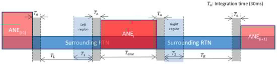
Figure 4.
An anomalous noise event is surrounded by road traffic or background noise. In this case both regions of RTN are balanced.
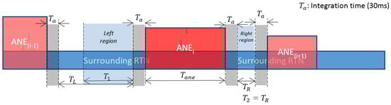
Figure 5.
An anomalous noise event surrounded by road traffic or background noise. In this second case, left region contains more samples than right region.
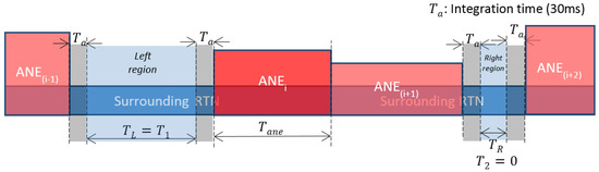
Figure 6.
Other noise events occur just before and/or after the analyzed anomalous noise event. Example where all the samples considered for the SNR computation come from the left region.
Contrary to the previous example, in Figure 5 an example where the right region does not contain enough samples to obtain a balanced set of time regions of surrounding RTN is shown. As a consequence, more samples from the left region are considered here for the SNR computation.
- Other anomalous noise events occur just before and/or after the analyzed anomalous noise event: In this less-frequent scenario, the selection of the time regions where the BCK or the RTN is computed is a little more intricate. The calculation process looks for the closest time regions to the current ANE following a global idea of measuring the contextual SNR with a proximity criterion, and trying to obtain as many samples of background or road traffic noise as the samples contained in the anomalous noise event duration (). In this case, the closest BCK or RTN region to the analyzed ANE is firstly considered. If the duration of this region is greater than and all its samples are closer to the analyzed ANE than any other sample from the opposite side, then the interval of duration is considered as closest to the analyzed ANE (being T the duration of this time region). Otherwise, when it is possible to obtain samples of BCK and/or RTN from both sides of the analyzed ANE with the general criterion that none of these two time regions are strictly closer to the ANE than the other due to the presence of other ANEs, then samples from both sides of the ANE are used to compute the BCK and/or RTN .
In Figure 6, an example of this kind of contextual SNR computation where all the samples come from the left region is shown. This is because the RTN samples in the right region are further away than the farthest sample of the RTN left region (then, ).
In Figure 7, three examples of the most usual ANE contextual SNR computation cases (i.e., an anomalous noise event surrounded by road traffic or background noise) are shown. The A-weighted curve is highlighted, representing the time region attributed to an anomalous noise event in red, and the background or road traffic noise in blue. A time period equal to the integration time for the computation is depicted in black at both sides of the anomalous event, in order to prevent transients affecting the SNR computation. The median for each time region are shown as magenta horizontal lines (for background and RTN at both sides) and horizontal red lines (for the ANE). Finally, the median of the surrounding background or road traffic noise considering both ANE sides is depicted as a green horizontal line within the ANE time region.
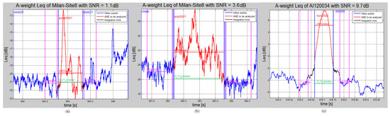
Figure 7.
Examples of SNR labeling of three anomalous noise events. From left to right: (a) a low-salient ANE (people talking in the street, measured in a Milan street, with SNR = 1.1 dB); (b) a medium-salient ANE (the sound of an airplane measured in another Milan road, with SNR = 3.6 dB); and (c) a high-salient ANE (sound of a horn measured along the A90 motorway in Rome, with SNR = 9.7 dB). x-axis corresponds to time in seconds referenced to the start point of the recording.
4. Analysis of the Anomalous Noise Events Present in the Urban and Suburban Environments
In this section, a detailed analysis of the anomalous noise events present in the labelled real-life audio database is described. Specifically, we study the distribution of the occurrences and durations of the ANE subcategories together with their contextual SNR distribution in both urban (Milan and suburban (Rome) scenarios. Some examples of representative ANEs extracted from both scenarios are included in Appendix A in order to show their values together with their spectro-temporal evolution for illustrative purposes.
4.1. ANE Occurrences
This first part of the study aims at determining the predominant types of ANE for each of the two recording scenarios. To that end, the ANEs distribution of occurrences is determined by computing the accumulated duration of each ANE subcategory within the real-life database. In Figure 8, the distributions of the sum of ANE durations are depicted. As it can be observed, sirens and sound of portals’ structures (‘stru’) followed by the noise of vehicle horns, people, trucks and car brakes are the most observed subcategories considered as anomalous noise events, being the rest significantly-less probable. As the list of anomalous events subcategories have been defined (see Section 3.2) to account for all types of ANEs recorded either in the urban or suburban environments, it can be also observed that some ANE subcategories do not occur in the suburban area. For instance, no samples of airplanes, bikes, birds, chains, dogs, mega, thunder, tramways or wind were recorded during the suburban real-life recordings. On the contrary, some types of anomalous noise events were collected unexpectedly in this environment. For instance, highway operators talking while doing maintenance works were recorded (i.e., ‘peop’ ANE subcategory), which is a somewhat rare event to collect in a suburban scenario such as a highway. As foreseen, a larger diversity of ANEs can be observed in the urban than in suburban soundscape.
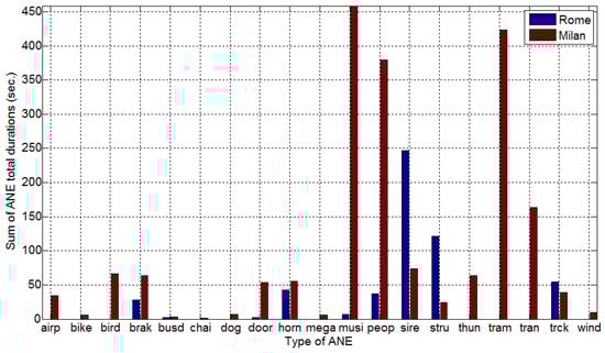
Figure 8.
Histograms showing the accumulated ANE durations per category differentiating both locations Rome (suburban) and Milan (urban). The x-axis show the ANE category.
Regarding the probability of the recorded ANEs, it can be concluded from Figure 8 that sirens and the sound of portal’s structures were the most frequent ANEs in the urban environment, while music, people talking and sounds of tramways and trains where the most represented events in the urban area. In a second order of occurrence, we can find brakes, horns, people talking and trucks in the suburban area, while in the urban context, sounds of airplanes, birdsongs, car brakes, doors, horns, sirens, structures, thunders and trucks can be observed. Finally, the less frequent sounds are sound of pressurized air (busd), door or impulsive-like sounds, and music in cars in the suburban soundscape, and sounds of bikes, opening bus or tramway door noises (busd), chains, dog’s barks, noise of people reporting by the public address station (mega), and wind in the urban sound field.
4.2. ANE Durations
In this section, we analyze the durations of the ANE subcategories for each of the two recording scenarios. In Figure 9 the boxplots of ANE durations are shown for each ANE subcategory. As it can be observed, in the suburban context the sounds of sirens constitute the longest ANEs, while the shortest ones are impulsive-like noises (labelled as ‘door’) in the A90 highway ring circumventing Rome. However, in these recordings brake noises, people, sounds of trucks and noise coming from the structure of portals also have significant durations.
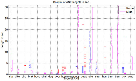
Figure 9.
Boxplots of the durations of each ANE type per category differentiating both locations Rome (suburban) and Milan (urban).
Regarding the audio recorded in urban area within district 9 of Milan, Figure 9 shows that music, sirens and tramways and trains, airplanes and wind sound are the ones with longer durations. We should underline the fact that in the context of an urban environment like the one in Milan, events like sirens exhibit larger durations than those observed in the Rome A90 highway, because vehicles speeds are lower and, as a consequence, the duration of the passing of the vehicles with respect to the point of measurement is longer.
4.3. ANE SNR Distributions
In this section, the analysis of the ANE contextual SNR is described with the aim of obtaining a more accurate understanding of the salience of anomalous noise events with respect to the surrounding road traffic noise in real-life scenarios. The boxplots of the measured SNR for each type of ANE collected in both urban and suburban locations are depicted in Figure 10.
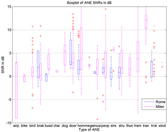
Figure 10.
Boxplots of contextual SNR for each ANE type in each of two site locations (urban: Milan and suburban:Rome).
Moreover, the majority of median SNR values are located in the range between 0 and dB, except for dog’s barks, sirens and trains in the urban scenario. The traffic density during the recordings in the suburban area was generally high or very high, which made it difficult to obtain audio passages where other types of noises surpassed significantly the background traffic noise (i.e., with high salience). The mean value of SNR for the observed anomalous noise events is dB and dB in the suburban and urban environments, respectively.
Door or impulsive-like sounds are the ANEs presenting a higher SNR in the suburban context, while in the urban one there is a more uniform distribution of ANEs entailing higher saliencies (i.e., dogs barking, horns, people, sirens, trams and trains and sounds of trucks). In this sense, several ANEs occurred in the urban area over quiet background noise conditions (labelled as BCK), making, for instance, that a dog’s barking became a salient ANEs as being recorded in one direction road with very low traffic conditions.
5. Discussion
In this section, several relevant aspects are discussed after the generation, annotation and analysis of the recorded database in real-life urban and suburban scenarios, paying special attention to what has been already considered in previous works. Moreover, some general implications derived from the obtained results are also presented to help the development of ANE databases for automatic detection systems in real-life urban and suburban environments.
5.1. Sensor Locations during the Recording Campaign
During the recording campaign, the sensors were placed at the portals of the highway in the suburban area, which is the exact position they will be installed for the WASN thanks to the collaboration of the DYNAMAP’s ANAS S.p.A partner. However, they were located at more than 2 m from the buildings in the urban scenario, which can differ from the positions where the WASN low-cost sensors will be placed when deploying the pilot system of the DYNAMAP project in Milan (e.g., fixed at the buildings façade). Moreover, also different elevation angles were considered in the sensors’ orientation during the recording campaign. At this point, an interesting question arises: To what extent do the position and orientation of the sensors influence aspects like acoustic salience of sound events and spectral content of sound or road traffic noise? More work needs to be done to answer these questions, e.g., by performing contrast analyses with the gathered measurements obtained with different sensors’ positions and orientations, beyond the preliminary comparisons already conducted.
5.2. Database Annotation
The labelling of the real-life audio database has undergone both manual and automatic processes. The manual labelling of the time boundaries of the audio scenes and events has guaranteed subsequent reliable analyses. However, since it is a burdensome and time consuming task, it may hinder the generation of new databases from field recordings. To alleviate this task, we can consider those approaches focused on the identification of salient audio events regardless of their origin (e.g., [24,25,26]) or semi-supervised techniques that combine confidence-based active learning and self-training [40], allowing the combination of automatic labelling (high confidence scores) and human annotation (when low scores are obtained). However, whichever the approach followed to cope with non-stationary background noise, it is envisioned as a very challenging task.
On the other hand, the acoustic salience of the anomalous noise events with respect to background noise has been automatically quantified in terms of SNR with higher resolution than in [34], where a binary salience descriptor was considered to differentiate between foreground and background noises. The computation of the ANE contextual SNR with respect to RTN or BCK noise levels poses several challenges. The RTN within the ANE time interval is computed by considering the surrounding samples, which entails a simplification due to the non-stationary nature of road traffic noise. In addition, during the ANE time interval, the measured is also influenced by background noise (this is of especially relevance for those ANE with low SNR). Moreover, real-life noise sources can exhibit relevant level variations along time. For instance, an ambulance passing by with siren generates a long sound with a high noise level when closest to the point of measurement, which then fades in the approaching and receding phases. Ideally, instead of only accounting for the mean SNR value, it would be desirable to obtain SNR labels at different time instants, considering the sound level trajectory of each sound source. This approach could be understood as a time-varying soft-salience labelling. From the ANE salience analysis, we have been provided with some relevant insights on what can be found in real-life urban and suburban environments. Any machine hearing running in real-life conditions should be designed to tackle the diversity of ANE in terms of salience, i.e., being robust to ANE salience variability.
Finally, it is worth mentioning that both the definition and the categories of anomalous noise events can be a matter of discussion. In this work, they have been agreed with the DYNAMAP project consortium, considering ANE to be those audio events that do not reflect regular road traffic noise [1], i.e., coming from vehicles’ engines or derived from the normal contact of their tires with the road surface. Nevertheless, both the definition and the list of ANE might be subject of modification in future works.
5.3. Implications of the Results
In general terms, the conducted statistical analyses confirm that the two chosen scenarios (urban and suburban) exhibit different patterns in terms of both background noise and anomalous noise events, e.g., showing significant differences in terms of types of ANE and SNRs between them; a result that could be expected a priori. However, beyond specific aspects related to the different characteristics of these soundscapes (e.g., the impulse-like vs. stationary nature of noise events), it is reasonably to remark that both soundscapes entail a large variability and diversity of ANE in terms of occurrences, durations and SNRs. Regarding background noise, the suburban recordings contain mainly continuous road traffic noise, while the urban recordings also include other kinds of road noise like those gathered from interrupted traffic (e.g., crossroad with traffic lights) or the background city noise observed in low-density traffic city roads. Concerning the ANEs, the urban scenario entails a larger diversity of anomalous noise events than the suburban scenario, while the latter presents ANEs with lower contextual SNRs.
Another interesting aspect derived from the analyses is that real-life recordings reflect a highly unbalanced nature between anomalous noise events (uncommon sounds) and road traffic or background city noise (common sounds). In the 9 h 8 min of labelled audio database, the ANE subset represents 3.2% of the total recorded audio in the suburban scenario, while in the urban soundscape it comprises 12.2%. This fact can be of paramount importance when it comes to developing sound event detectors or classifiers, as the training and testing processes can be highly influenced by the ratio between the amount of examples of the classes to be identified [28,41]. Furthermore, the limited presence of ANEs in real-life recordings also makes it very difficult to model of such diversity of sound events within individual classes (i.e., one class per event typology). This issue can be alleviated by integrating all types of ANE within the same class, as will be done in the DYNAMAP project to discard them from the road traffic noise computation.
Furthermore, we can also conclude that the generation of synthetic sound mixtures either from online databases or real isolated ANE by considering predefined SNRs as proposed in previous works is still far from what can be observed in both real-life urban and suburban scenarios, which entail a dramatically larger variability. Concretely, ANE variability has been observed both in terms of the number of occurrences per ANE and the diversity of their durations, ranging from almost 0 s for impulse-like sounds such as dogs barks or closing vehicle doors, to more than 30 s for music or sirens. Moreover, the mean SNR values in both real-life urban and suburban recordings also show a significantly larger range of values (from to dB) with respect to previous artificially generated audio databases (e.g., dB [22] or dB plus dB [21]), with relevant diversity of intermediate SNR values. In our opinion, this fact is of paramount importance since the acoustic salience of a sound event could highly affect the performance of any automatic recognition system as already observed in [28]. However, this hypothesis should be further studied in future works.
Finally, although the recording campaign was designed to collect a large diversity of anomalous noise events, it is worth mentioning that the obtained results should not be understood as a generalizable result to any urban or suburban scenario as the recorded database comprises a large but limited set of labelled audio recordings of 9 h 8 min. At best, the obtained general patterns could be observed in very similar urban and suburban environments. Nevertheless, the main conclusions and considerations discussed in this paper can be taken into consideration for similar studies. For instance, from these results, it seems reasonable to avoid characterizing both acoustic environments altogether when it comes to developing the signal processing techniques run at the WASN acoustic sensors. On the contrary, characterizing each type of soundscape independently seems more appropriate. However, the latter approach make the scalability of the system more difficult and costly. Therefore, further studies should be conducted in order to find some trade-off between a general machine hearing system and a specifically trained system for each WASN sensor location.
6. Conclusions
This work has presented the production and analysis of a real-life environmental audio database in two urban and suburban scenarios corresponding to the pilot areas of the DYNAMAP project: the Milan district 9 and the Rome A90 highway, respectively. The collected 9 h 8 min of audio data have been categorized as road traffic noise, background city noise, and anomalous noise events. Due to the relevance of the ANE for the generation of reliable traffic noise maps through WASN, that category has been subsequently annotated using 19 subcategories and automatically labelled in terms of contextual acoustic salience as signal-to-noise ratio.
The in-depth analysis of the distribution of the ANEs collected in the database has shown the high diversity of ANE in terms of occurrence, duration and salience, besides confirming their local and occasional nature. Although, as expected beforehand, specific differences have been found between both soundscapes due to their specific acoustic nature, both environments show high ANE diversity, besides presenting a dramatically large range and variation of SNR values when compared to previous artificially generated ANE audio databases. The obtained results have been also comprehensively discussed to guide the development of automatic ANE classifiers using real-life environmental data in future works, by accounting for the implications of this kind of peculiar acoustic data.
Finally, we do not discard extending the conducted analyses in the considered urban and suburban soundscapes along with the DYNAMAP’s WASN deployment in order to include a larger diversity of weather and traffic conditions, compare the obtained results with the final location of the low-cost sensors in the urban environment, etc., besides studying in more detail those audio clips tagged as ‘complex audio’. Moreover, we also plan to analyze the statistical differences between ANE and road traffic or background noise at the spectral level for the future development of anomalous noise event detection systems in both scenarios.
Acknowledgments
This research has been partially funded by the European Commission under project LIFE DYNAMAP LIFE13 ENV/IT/001254 and the Secretaria d’Universitats i Recerca del Departament d’Economia i Coneixement (Generalitat de Catalunya) under grant ref. 2014-SGR-0590. We would like to thank our colleagues in ANAS S.p.A., Bluewave and Università di Milano-Bicocca for their support during the recording campaign.
Author Contributions
The authors contributed equally to this work. Francesc Alías led the initiative of preparing and writing the manuscript, also defining the focus of the analysis process, while Joan Claudi Socoró led the production and analysis of the environmental audio database, besides to also contributing to the writing of the paper.
Conflicts of Interest
The authors declare no conflict of interest.
Abbreviations
The following abbreviations are used in this manuscript:
| ANE | Anomalous Noise Event |
| ANED | Anomalous Noise Event Detection |
| BCK | Background noise |
| DYNAMAP | Dynamic Noise Mapping project |
| GTCC | Gammatone Cepstral Coefficients |
| RTN | Road Traffic Noise |
| SNR | Signal-to-Noise ratio |
Appendix A
In this section, some representative examples of anomalous noise events selected from both scenarios (urban and suburban) are shown in terms of their spectral and behaviours for illustrative purposes. The purpose of the following examples is to show that real-life recordings poses a serious challenge for ensuring a reliable database labelling process. In the following examples, the A-weighted equivalent noise level using 30 ms as integration time () is computed. Also, perceptual-based spectrograms are derived from the Gammatone Cepstral Coefficients (GTCC) parameterization of the input audio signal, by using a Gammatone filterbank of 48 subbands within the available frequency range at 48 KHz, a frame length of 30 ms with Hamming window and with overlap of 50% between consecutive frames [42]. In the figures, the ANEs start and end time boundaries are represented as magenta vertical dashed lines, and their labels and SNRs obtained from the labelling process described in Section 3.3 are also superimposed in both curves and spectrograms.
In Figure A1, an example of different ANEs recorded in the Milan urban environment is depicted. The recording was obtained in a two-way street with two lanes each way in the Milan city center, specifically close to the traffic lights of a crossroad and within a shopping area. As it can be observed, the excerpt covers up to 14 s of audio in which four types of anomalous noise events are highlighted: two events of people talking (‘peop’), a car horn (‘horn’), three door-like sound (‘door’) and a car brake (‘brak’). Four ANEs with low (or very low) saliency can be observed: the car brake sound (SNR dB) two doors (SNRs of and dB) and one sound of people talking (SNR dB). Also two intermediate saliency ANEs (people sound event with SNR dB and a door sound with SNR dB) and a high saliency ANE can be seen (car horn with SNR dB). In this example almost all the ANEs are quite identifiable directly from the trajectory: there is a clear pulse-like waveform that comprises the main parts of the ANE, which emphasizes its salience with respect to the background traffic noise. However, the non-stationary nature of the sound sources poses a challenge to compute the ANE contextual SNR reliably. In the case of sound of people talking, vowels usually have a higher than consonants. Contrarily, door-like sounds are very impulsive and their acoustic energy is highly local.
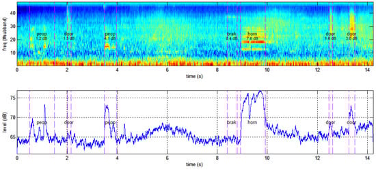
Figure A1.
Example with up to seven ANEs obtained in a two-way street with two lanes each way in the urban scenario (city center of Milan). GTCC-based spectrogram (upper) and A-weighted equivalent noise levels (bottom) are shown.
In Figure A2, another example of two ANEs with different salience (intermediate and high) observed in the urban scenario within a low traffic density one-way little road in Milan is shown. Their respective SNRs are shown under their four-character label (‘airp’ and ‘tran’). As it can be observed, two cars pass-bys are present between the two ANEs, which constitutes a highly non-stationary background. In this example, it is evident that traffic noise and the two ANEs exhibit trajectories that can be hardly distinguished, while GTCC-based spectral distributions could contribute to better represent their differences.
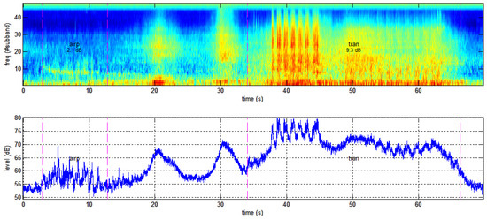
Figure A2.
Examples of a mid-salient ANE (airplane, with SNR dB) and a highly-salient ANE (train, with SNR dB) in the urban scenario. Recordings were obtained in a one-way little road with very low traffic density and near a railway in Milan. GTCC-based spectrogram (upper) and A-weighted equivalent noise levels (bottom) are shown.
Figure A3 shows an example of anomalous noise events with intermediate, low or very low saliency and road traffic noise +collected in the suburban scenario (Rome ring highway). Two sirens are observed with different SNRs ( and dB), also two horns with different SNRs ( and dB) and the sound of portal structure movement when a big truck pass-by (with SNR = dB). Compared to the previous examples recorded in Milan’s urban scenario, in this example the analyzed ANEs contextual SNRs present lower values. While the two ANEs with highest SNR (first siren and first horn) can be identified from the curve, the other three events with low or very low saliency remain quite unnoticed.
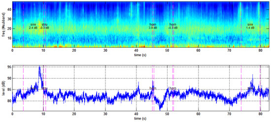
Figure A3.
Examples of sirens, horns and sound of portal structure when a big truck passby in the Rome ring highway. GTCC-based spectrogram (upper) and A-weighted equivalent noise level (bottom) are shown.
References
- Environmental Noise Directive (END). Directive 2002/49/EC of the European Parliament and the Council of 25 June 2002 relating to the assessment and management of environmental noise. Off. J. Eur. Commun. 2002, L189, 12–26. [Google Scholar]
- Bertrand, A. Applications and trends in wireless acoustic sensor networks: A signal processing perspective. In Proceedings of the 18th IEEE Symposium on Communications and Vehicular Technology in the Benelux (SCVT), Ghent, Belgium, 22–23 November 2011; IEEE: New York, NY, USA, 2011; pp. 1–6. [Google Scholar]
- Simon, G.; Maróti, M.; Lédeczi, A.; Balogh, G.; Kusy, B.; Nádas, A.; Pap, G.; Sallai, J.; Frampton, K. Sensor Network-based Countersniper System. In Proceedings of the 2nd International Conference on Embedded Networked Sensor Systems, Baltimore, MD, USA, 3–5 November 2004; ACM: New York, NY, USA, 2004; pp. 1–12. [Google Scholar]
- Paulo, J.; Fazenda, P.; Oliveira, T.; Carvalho, C.; Félix, M. Framework to monitor sound events in the city supported by the FIWARE platform. In Proceedings of the TecniAcústica 2015—46th Spanish Congress on Acoustics, Valencia, Spain, 21–23 October 2015; SEA: Madrid, Spain, 2015; pp. 387–396. [Google Scholar]
- Foggia, P.; Petkov, N.; Saggese, A.; Strisciuglio, N.; Vento, M. Audio Surveillance of Roads: A System for Detecting Anomalous Sounds. IEEE Trans. Intell. Transp. Syst. 2016, 17, 279–288. [Google Scholar] [CrossRef]
- Manvell, D. Utilising the Strengths of Different Sound Sensor Networks in Smart City Noise Management. In Proceedings of the EuroNoise 2015, Maastrich, The Netherlands, 31 May–3 June 2015; EAA-NAG-ABAV: Madrid, Spain, 2015; pp. 2305–2308. [Google Scholar]
- Nencini, L.; Rosa, P.D.; Ascari, E.; Vinci, B.; Alexeeva, N. SENSEable Pisa: A wireless sensor network for real-time noise mapping. In Proceedings of the EuroNoise Conference, Prague, Czech Republic, 10–13 June 2012; Volume 12.
- Botteldooren, D.; De Coensel, B.; Oldoni, D.; Van Renterghem, T.; Dauwe, S. Sound monitoring networks new style. In Acoustics 2011: Breaking New Ground, Proceedings of the Annual Conference of the Australian Acoustical Society, Gold Coast, Australia, 2–4 November 2011; Mee, D.J., Hillock, I.D., Eds.; Australian Acoustical Society: Queensland, Australia, 2011; pp. 93:1–93:5. [Google Scholar]
- Mietlicki, F.; Mietlicki, C.; Sineau, M. An innovative approach for long-term environmental noise measurement: RUMEUR network. In Proceedings of the EuroNoise 2015, Maastrich, The Netherlands, 31 May–3 June 2015; EAA-NAG-ABAV: Madrid, Spain, 2015; pp. 2309–2314. [Google Scholar]
- Camps, J. Barcelona noise monitoring network. In Proceedings of the EuroNoise 2015, Maastrich, The Netherlands, 31 May–3 June 2015; EAA-NAG-ABAV: Madrid, Spain, 2015; pp. 2315–2320. [Google Scholar]
- Sevillano, X.; Socoró, J.C.; Alías, F.; Bellucci, P.; Peruzzi, L.; Radaelli, S.; Coppi, P.; Nencini, L.; Cerniglia, A.; Bisceglie, A.; et al. DYNAMAP—Development of low cost sensors networks for real time noise mapping. Noise Mapp. 2016, 3, 172–189. [Google Scholar] [CrossRef]
- De la Piedra, A.; Benitez-Capistros, F.; Dominguez, F.; Touhafi, A. Wireless sensor networks for environmental research: A survey on limitations and challenges. In Proceedings of the 2013 IEEE EUROCON, Zagreb, Croatia, 1–4 July 2013; IEEE: New York, NY, USA, 2013; pp. 267–274. [Google Scholar]
- Rawat, P.; Singh, K.D.; Chaouchi, H.; Bonnin, J.M. Wireless Sensor Networks: A Survey on Recent Developments and Potential Synergies. J. Supercomput. 2014, 68, 1–48. [Google Scholar] [CrossRef]
- Griffin, A.; Alexandridis, A.; Mastorakis, D.P.Y.; Mouchtaris, A. Localizing multiple audio sources in a wireless acoustic sensor network. Signal Process. 2015, 107, 54–67. [Google Scholar] [CrossRef]
- Giannoulis, D.; Stowell, D.; Benetos, E.; Rossignol, M.; Lagrange, M.; Plumbley, M.D. A database and challenge for acoustic scene classification and event detection. In Proceedings of the 21st European Signal Processing Conference (EUSIPCO 2013), Marrakech, Morocco, 9–13 September 2013; IEEE: New York, NY, USA, 2013; pp. 1–5. [Google Scholar]
- Heittola, T.; Mesaros, A.; Eronen, A.; Virtanen, T. Context-dependent sound event detection. EURASIP J. Audio Speech Music Process. 2013, 2013. [Google Scholar] [CrossRef]
- Mesaros, A.; Heittola, T.; Virtanen, T. Metrics for Polyphonic Sound Event Detection. Appl. Sci. 2016, 6, 162. [Google Scholar] [CrossRef]
- Wang, D.; Brown, G.J. Computational Auditory Scene Analysis: Principles, Algorithms, and Applications; Wiley-IEEE Press: Hoboken, NJ, USA, 2006. [Google Scholar]
- Foggia, P.; Petkov, N.; Saggese, A.; Strisciuglio, N.; Vento, M. Reliable detection of audio events in highly noisy environments. Pattern Recognit. Lett. 2015, 65, 22–28. [Google Scholar] [CrossRef]
- Mesaros, A.; Heittola, T.; Virtanen, T. TUT database for acoustic scene classification and sound event detection. In Proceedings of the 24th European Signal Processing Conference, Budapest, Hungary, 29 August–2 September 2016; IEEE: New York, NY, USA, 2016; Volume 2016, pp. 1128–1132. [Google Scholar]
- Socoró, J.C.; Ribera, G.; Sevillano, X.; Alías, F. Development of an Anomalous Noise Event Detection Algorithm for dynamic road traffic noise mapping. In Proceedings of the 22nd International Congress on Sound and Vibration (ICSV22), Florence, Italy, 12–16 July 2015; The International Institute of Acoustics and Vibration (IIAV): Auburn, AL, USA, 2015; pp. 1–8. [Google Scholar]
- Nakajima, Y.; Sunohara, M.; Naito, T.; Sunago, N.; Ohshima, T.; Ono, N. DNN-based Environmental Sound Recognition with Real-Recorded and Artificially-mixed Training Data. In Proceedings of the 45th International Congress and Exposition on Noise Control Engineering (InterNoise 2016), Hamburg, Germany, 21–24 August 2016; German Acoustical Society (DEGA): Berlin, Germany, 2016; pp. 3164–3173. [Google Scholar]
- Mesaros, A.; Heittola, T.; Eronen, A.; Virtanen, T. Acoustic event detection in real life recordings. In Proceedings of the 2010 18th European Signal Processing Conference, Aalborg, Denmark, 23–27 August 2010; IEEE: New York, NY, USA, 2010; pp. 1267–1271. [Google Scholar]
- De Coensel, B.; Botteldooren, D. A model of saliency-based auditory attention to environmental sound. In Proceedings of the 20th International Congress on Acoustics (ICA 2010), Sydney, Australia, 23–27 August 2010; Curran Associates, Inc.: New York, NY, USA, 2010; pp. 3480–3487. [Google Scholar]
- Zlatintsi, A.; Maragos, P.; Potamianos, A.; Evangelopoulos, G. A saliency-based approach to audio event detection and summarization. In Proceedings of the 2012 Proceedings of the 20th European Signal Processing Conference (EUSIPCO), Bucharest, Romania, 27–31 August 2012; IEEE: New York, NY, USA, 2012; pp. 1294–1298. [Google Scholar]
- Schauerte, B.; Stiefelhagen, R. Wow! Bayesian surprise for salient acoustic event detection. In Proceedings of the 2013 IEEE International Conference on Acoustics, Speech and Signal Processing, Vancouver, BC, Canada, 26–31 May 2013; IEEE: New York, NY, USA, 2013; pp. 6402–6406. [Google Scholar]
- Gloaguen, J.R.; Can, A.; Lagrange, M.; Petiot, J.F. Estimating Traffic Noise Levels using Acoustic Monitoring: A Preliminary Study. In Proceedings of the Detection and Classification of Acoustic Scenes and Events 2016 (DCASE’2016), Budapest, Hungary, 3 September 2016; Department of Signal Processing, Tampere University of Technology: Tampere, Finland, 2016; pp. 40–44. [Google Scholar]
- Socoró, J.C.; Albiol, X.; Sevillano, X.; Alías, F. Analysis and automatic detection of anomalous noise events in real recordings of road traffic noise for the LIFE DYNAMAP project. In Proceedings of the 45th International Congress and Exposition on Noise Control Engineering (InterNoise 2016), Hamburg, Germany, 21–24 August 2016; German Acoustical Society (DEGA): Berlin, Germany, 2016; pp. 6370–6379. [Google Scholar]
- Stowell, D.; Plumbley, M.D. An open dataset for research on audio field recording archives: Freefield1010. arXiv 2013. [Google Scholar]
- Piczak, K.J. ESC: Dataset for Environmental Sound Classification. In Proceedings of the 23rd ACM International Conference on Multimedia, Brisbane, Australia, 26–30 October 2015; ACM: New York, NY, USA, 2015; pp. 1015–1018. [Google Scholar]
- Temko, A. Acoustic Event Detection and Classification. Ph.D. Thesis, Universitat Politècnica de Catalunya, Barcelona, Spain, 2007. [Google Scholar]
- Stowell, D.; Giannoulis, D.; Benetos, E.; Lagrange, M.; Plumbley, M.D. Detection and Classification of Acoustic Scenes and Events. IEEE Trans. Multimed. 2015, 17, 1733–1746. [Google Scholar] [CrossRef]
- Alías, F.; Socoró, J.C.; Sevillano, X. A Review of Physical and Perceptual Feature Extraction Techniques for Speech, Music and Environmental Sounds. Appl. Sci. 2016, 6, 143. [Google Scholar] [CrossRef]
- Salamon, J.; Jacoby, C.; Bello, J.P. A dataset and taxonomy for urban sound research. In Proceedings of the 22nd ACM International Conference on Multimedia, Orlando, FL, USA, 3–7 November 2014; ACM: New York, NY, USA, 2014; pp. 1041–1044. [Google Scholar]
- Rossignol, M.; Lafay, G.; Lagrange, M.; Misdariis, N. SimScene: A web-based acoustic scenes simulator. In Proceedings of the 1st Web Audio Conference (WAC), IRCAM & Mozilla, Paris, France, 26–27 January 2015; IRCAM: Paris, France, 2015; pp. 1–6. [Google Scholar]
- Radaelli, S.; Coppi, P.; Giovanetti, A. The LIFE DYNAMAP PROJECT: Automating the process for pilot areas location. In Proceedings of the 22nd International Congress on Sound and Vibration (ICSV22), Florence, Italy, 12–16 July 2015; The International Institute of Acoustics and Vibration (IIAV): Auburn, AL, USA, 2015; pp. 1–8. [Google Scholar]
- Zambon, G.; Benocci, R.; Bisceglie, A. Development of optimized algorithms for the classification of networks of road stretches into homogeneous clusters in urban areas. In Proceedings of the 22nd International Congress on Sound and Vibration, Florence, Italy, 12–16 July 2015.
- Nencini, L. DYNAMAP monitoring network hardware development. In Proceedings of the 22nd International Congress on Sound and Vibration (ICSV22), Florence, Italy, 12–16 July 2015; The International Institute of Acoustics and Vibration (IIAV): Auburn, AL, USA, 2015; pp. 1–4. [Google Scholar]
- Alías, F.; Socoró, J.C.; Sevillano, X.; Nencini, L. Training an Anomalous Noise Event Detection Algorithm for Dynamic Road Traffic Noise Mapping: Environmental Noise Recording Campaign. In Proceedings of the TecniAcústica 2015—46th Spanish Congress on Acoustics, Valencia, Spain, 21–23 October 2015; SEA: Madrid, Spain, 2015; pp. 345–352. [Google Scholar]
- Han, W.; Coutinho, E.; Ruan, H.; Li, H.; Schuller, B.; Yu, X.; Zhu, X. Semi-Supervised Active Learning for Sound Classification in Hybrid Learning Environments. PLoS ONE 2016, 11, 1–23. [Google Scholar] [CrossRef] [PubMed]
- Hoens, T.R.; Chawla, N.V. Imbalanced Datasets: From Sampling to Classifiers. In Imbalanced Learning; John Wiley & Sons, Inc.: Hoboken, NJ, USA, 2013; pp. 43–59. [Google Scholar]
- Valero, X.; Alías, F. Gammatone Cepstral Coefficients: Biologically Inspired Features for Non-Speech Audio Classification. IEEE Trans. Multimed. 2012, 14, 1684–1689. [Google Scholar] [CrossRef]
© 2017 by the authors. Licensee MDPI, Basel, Switzerland. This article is an open access article distributed under the terms and conditions of the Creative Commons Attribution (CC BY) license ( http://creativecommons.org/licenses/by/4.0/).