1. Introduction
The Hammond tonewheel organ is a classic electromechanical musical instrument, patented by Laurens Hammond in 1934 [
1]. Although it was intended as an affordable substitute for church organs [
2], it has also become widely known as an essential part of jazz (where it was popularized by Jimmy Smith), R & B and rock music (where the Hammond playing of Keith Emerson of Emerson, Lake & and Palmer and Jon Lord of Deep Purple is exemplary). The most popular model is the Hammond B-3, although many other models exist [
3]. The sound of the Hammond organ is rich and unusual. Its complexity comes from the Hammond organ’s unique approach to timbre and certain quirks of its construction.
In this article, we describe a novel class of modal-processor-based audio effects which we call the “Hammondizer”. The Hammondizer can imprint the sonics of the Hammond organ onto any sound; it mimics and draws inspiration from the architecture of the Hammond tonewheel organ. We begin by describing the architecture and sonics of the Hammond tonewheel organ alongside related work on Hammond organ modeling.
The Hammond organ is essentially an additive synthesizer. Additive synthesizers create complex musical tones by adding together sinusoidal signals of different frequencies, amplitudes, and phases [
4]. In the Hammond organ, 91 sinusoidal signals are available. These sinusoids are created when “tonewheels”—ferromagnetic metal discs—spin and the pattern of ridges cut into their edges is transduced by electromagnetic pickups into electrical signals, a technique originated in Thaddeus Cahill’s late-19th century instrument, the Telharmonium [
5]. Hammond organ tonewheel pickups have not been studied much in particular, but modeling and simulation of electromagnetic pickups in general is an active research area [
6,
7,
8,
9,
10]. Any nonlinearities in a pickup model will cause bandwidth expansion and add to the characteristic sound of the Hammond organ. In the case that this bandwidth expansion would go beyond the Nyquist limit, alias-suppression methods become relevant [
11,
12,
13,
14].
These 91 tonewheels are tuned approximately to the twelve-tone equal-tempered musical scale [
15]—In scientific pitch notation, the lowest-frequency tonewheel on a Hammond organ is tuned to C1 (
Hz) and the highest-frequency tonewheel is tuned to F#7 (
Hz) [
16]. The lowest octave of tonewheels do not form sinusoids, but more complex tones that have strong 3rd and 5th harmonics, making them closer to square waves than sine waves [
15]. Some aficionados have pointed to crosstalk between nearby tonewheel/pickup pairs as an important sonic feature of the Hammond organ [
17,
18].
The tone of the Hammond organ is set using nine “drawbars”. Unlike traditional organs, where “stops” bring in entire complex organ sounds, the Hammond organ’s drawbars set the relative amplitudes of individual sinusoids in a particular timbre. These nine sinusoids form a pseudo-harmonic series summarized in
Table 1 [
19]. This pseudo-harmonic series deviates from the standard harmonic series in three ways: (1) each overtone is tuned to the nearest available tonewheel; (2) certain overtones are omitted, especially the 6th harmonic, which would be between the 8th and 9th drawbar); and (3) new fictitious overtones are added (the 5th and sub-octave).
The raw sound of the Hammond organ tonewheels is static. To enrich the sound, Hammond added a chorus/vibrato circuit [
20]. Earlier models used a tremolo effect in place of the chorus/vibrato circuit [
21]. The sound was further enriched by an electro-mechanical spring reverb device [
22]. Although Hammond did not originally approve of the practice, it became customary to play Hammond organs through a Leslie speaker, an assembly with a spinning horn and baffle that creates acoustic chorus and tremolo effects. The Leslie speaker has been covered extensively in the modeling literature. Various approaches have involved interpolating delay lines [
23,
24] and amplitude modulation [
25,
26], perception-based models [
28], and time-varying Finite Impulse Response (FIR) filters [
29]. Recently, Pekonen et al. presented a novel Leslie model [
18] using spectral delay filters [
30]. Werner et al. used the Wave Digital Filter approach to model the Hammond vibrato/chorus circuit [
31].
Although Hammond had stopped manufacturing their tonewheel organs by 1975, the Hammond sound remained influential. Many manufacturers developed clones of the Hammond tonewheel organ [
17,
32,
33,
34,
35]. Commercial efforts have been accompanied by popular and academic work in virtual analog modeling [
36]. Gordon Reid wrote a series of articles for
Sound on Sound on generic synthesis approaches to modeling aspects of the Hammond organ [
17,
32,
33,
34,
35]. Pekonen et al. studied efficient methods for digital tonewheel organ synthesis [
18].
The Hammondizer audio effect is implemented as an extension to the recently-introduced “modal reverberator” approach to artificial reverberation [
37,
38,
39,
40]. Although there are many other approaches to modal sound synthesis in the literature (e.g., [
41,
42,
43,
44], the choice to extend the modal reverberator architecture to create the Hammondizer effect was a natural one for two reasons: (1) there are strong similarities between the system architecture of the Hammond organ and the system architecture of the modal reverberator; (2) the modal reverberator is already formulated as an audio effect which processes rather than synthesizes sound.
The rest of the article is structured as follows.
Section 2 presents a simplified system architecture of the Hammond organ,
Section 3 reviews relevant aspects of the modal processor approach,
Section 4 presents the novel Hammondizer digital audio effect,
Section 5 demonstrates features of the Hammondizer through a series of examples, and
Section 6 concludes.
2. Hammond Organ System Architecture
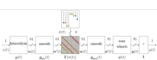
Here we extend the qualitative description above and present a mathematical formulation of the basic operation of the Hammond tonewheel organ. Referring to
Figure 1, the player controls the organ by depressing keys on a standard musical keyboard shown on the left. Each of its 61 keys has a note on/off state
that is indexed by a key number
; these are collected into a column
. Here and in the rest of the article,
t is the discrete time sample index.
The timbre is controlled by nine drawbars shown on the top. Each drawbar has a level
that is indexed by a drawbar number
; these are collected into a column
. The drawbars may be changed over time to alter the sounds of the Hammond organ. Each drawbar’s level
is converted to an amplitude in
dB increments (
Table 2) [
45].
Furthermore, each drawbar has a tuning offset
, corresponding to the tuning offset in semitones of each pseudo-harmonic. The entire set of offsets is
Each tuning offset (except the first two) approximates a harmonic overtone. This is discussed further at the end of the section.
Each tonewheel has a frequency
and amplitude
indexed by a tonewheel number
; these are collected into columns
and
. Each tonewheel is tuned to the twelve-tone equal-tempered scale
In practice there are slight deviations according to the gearing ratios, producing deviations of up to
cents [
15].
The outputs of all the tonewheels are summed by the
gain block
on the right to form the output signal
:
The
routing matrix
forms the 91-tall column of tonewheel amplitudes
from the 61-tall column of key on/off states
. This is accomplished by a matrix multiply
is sparse (most entries are 0) and has a pseudo-convolutional form [
46] in which the non-zero entries
are dictated by the 9-tall column of drawbar levels
. Denoting each entry in
as
, we have
where
is the Kronecker delta function
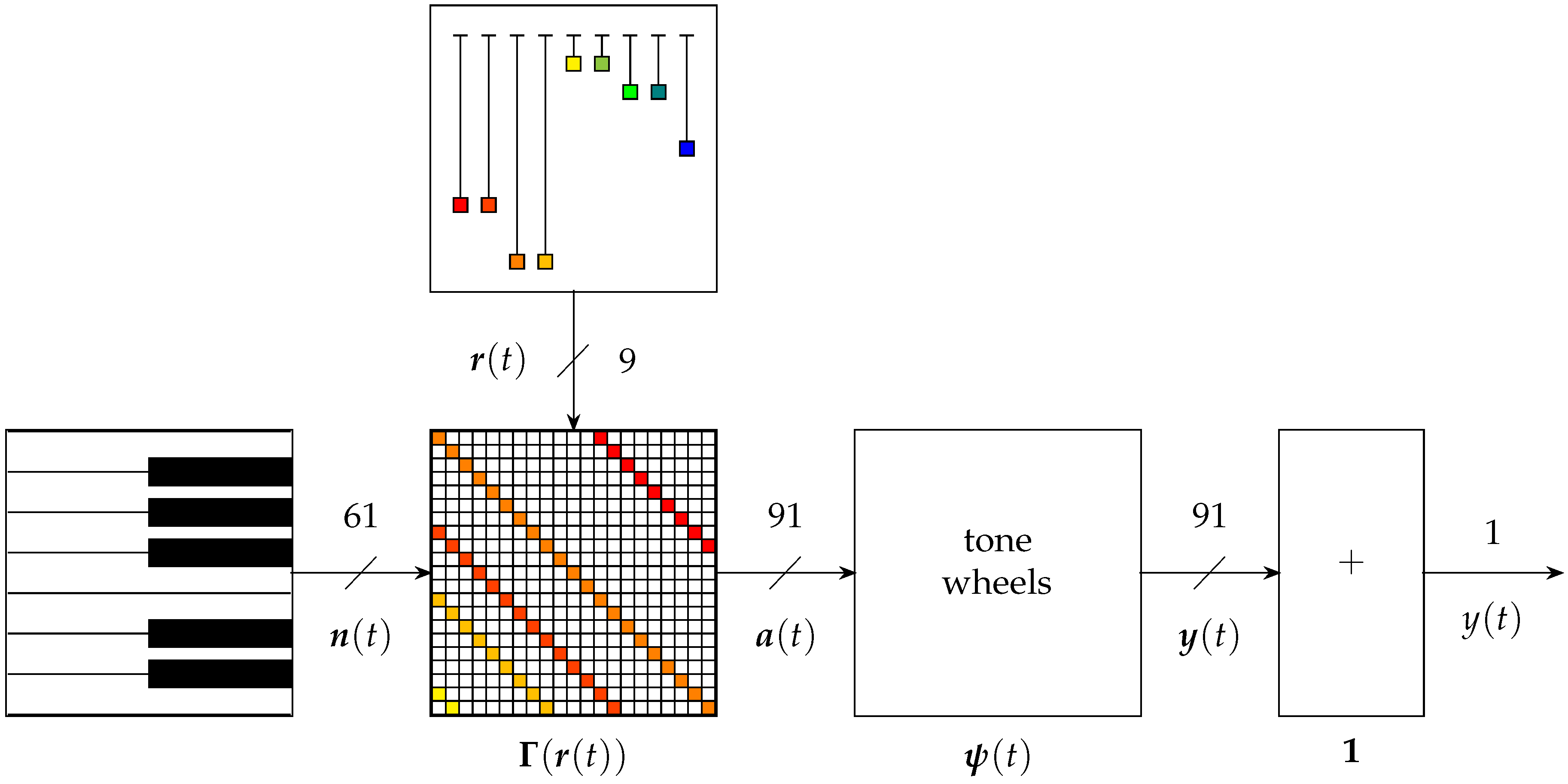
The tonewheel block is comprised of 91 tonewheel processors
in parallel. As shown in
Figure 2, each individual tonewheel processor has a tonewheel producing a periodic signal
at a particular frequency
, an amplitude input
provided by the routing matrix
, and an electromagnetic model
. Each tonewheel processor forms an output
by
A block diagram of an individual tonewheel processor is shown in
Figure 2. The matrix equation describing the entire bank of tonewheels is
where ⊙ is the Hadamard (elementwise) product operator
where
denotes the
th element of the matrix
.
The lowest 12 tonewheels produce roughly square-wave signals and the rest produce essentially sinusoidal signals:
As a final note, we can discuss the pseudo overtone series of the Hammond organ in more detail. Equation (
5) implies a certain relationship between any pressed key
k and the set of frequencies that are produced. Here we state this relationship explicitly. Given Equations (
1), (
2) and (
5), we can see that pressing any key
k will, in general, drive a set of nine tonewheels with frequencies
Most wind and string instruments are characterized by a harmonic overtone series—i.e., one where overtone frequencies are integer multiples of a fundamental frequency. Most of the tonewheel frequencies given in Equation (
11) approximate idealized harmonic overtones with frequencies given by
The first two tonewheel frequencies and are the octave below the fundamental frequency and approximately a fourth below the fundamental frequency—they are not approximations of standard harmonic overtones.
In general,
. The error in “cents” (
of a semitone) is given by
The tuning error of each tonewheel frequency is independent of
k; it depends only on the drawbar index
d—i.e., which overtone it is supposed to be approximating. These errors are given for each drawbar in
Table 1. For the fundamental and octave overtones, the tonewheels are perfectly in tune. For the 12th and 19th, the tonewheels are
cents flat of the ideal overtones. The 19th is
cents sharp. This detuning is very unique to the Hammond organ.
3. Modal Processor Review
The Hammondizer effect involves decomposing an input signal into a parallel set of narrow-band signals, analogous to a bank of organ keys. Each of the “keys” is then pitch processed according to the drawbar settings, and distortion processed according to the tonewheel and pickup mechanics and electromagnetics. It turns out that this structure closely resembles that of the modal reverberator [
37,
38], which forms a room response as the parallel combination of room vibrational mode responses. In the following, we review the modal reverberator and adapt it to produce the needed pitch and distortion processing.
The impulse response
between a pair of points in an acoustic space may be expressed as the linear combination of normal mode responses [
47,
48],
where the system has
M modes, with the
mth mode response denoted by
. The system output
in response to an input
, the convolution
, is therefore the sum of mode outputs
where the
mth mode output
is the
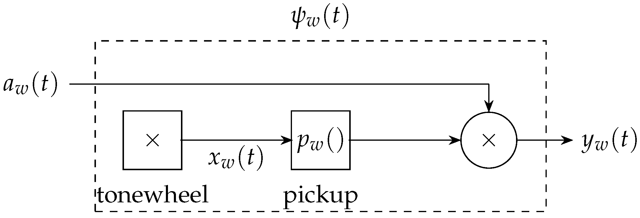
mth mode response convolved with the input. The modal reverberator simply implements this parallel combination of mode responses (
15), as shown in
Figure 3. Denoting by
the
M-tall column of complex mode responses, we have
with
and where convolution here obeys the rules of matrix multiplication, with each individual matrix operation replaced by a convolution.
The mode responses
are complex exponentials, each characterized by a mode frequency
, mode damping
, and mode complex amplitude
,
The mode frequencies and dampings are properties of the room or object; the mode amplitudes are determined by the sound source and listener positions (driver and pick-up positions for an electro-mechanical device), according to the mode spatial patterns.
Rearranging terms in the convolution
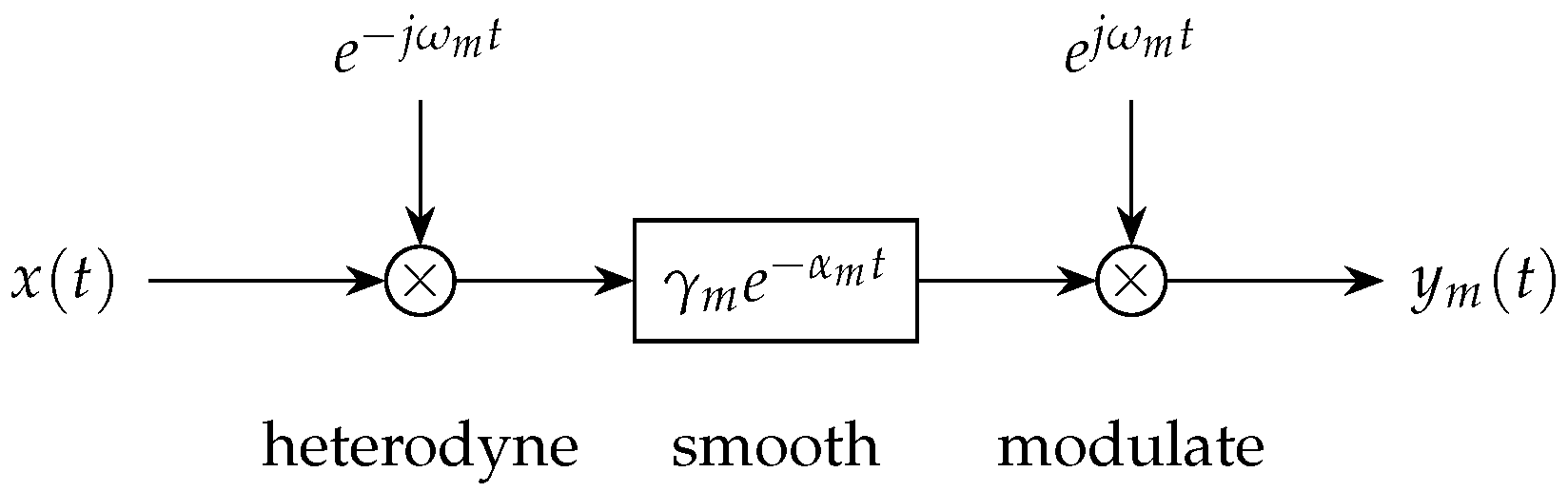
, the mode filtering is seen to heterodyne the input signal to dc to form a baseband response, smooth this baseband response by convolution with an exponential, and modulate the result back to the original mode frequency,
All
M γs are stacked into a diagonal gain matrix
Γ. All the heterodyning sinusoids are stacked into a column
, and all of the modulating sinusoids into a column
. The mode damping filters are stacked into a column
. This process is shown in
Figure 4. The heterodyning and modulation steps implement the mode frequency, and the smoothing filter generates the mode envelope, an exponential decay.
Using this architecture, rooms and objects may be simulated by tuning the filter resonant frequencies and dampings to the corresponding room or object mode frequencies and decay times. The parallel structure allows the mode parameters to be separately adjusted, while Equation (
19) provides interactive parameter control with no computational latency.
As described in [
39], the modal reverberator architecture can be adapted to produce pitch shifting by using different sinusoid frequencies for the heterodyning and modulation steps in Equation (
19), and adapted to produce distortion effects by inserting nonlinearities on the output of each mode or group of modes. The modal processor architecture has been used for other effects, including mode-wise gated reverb using Truncated Infinite Impulse Response (TIIR) filters [
49], groupwise distortion, time stretching by resampling of the baseband signals, and manipulation of mode time envelopes by introducing repeated poles [
39].
4. Hammondizer Modal Processor Implementation
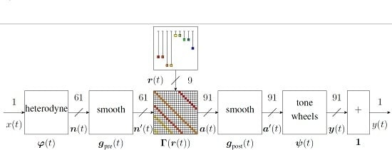
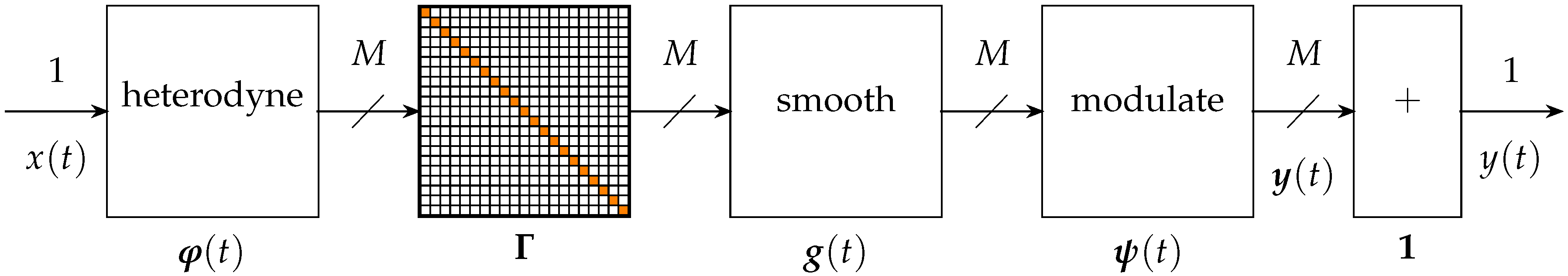
The Hammondizer effect system architecture is shown in
Figure 5. It turns out that this structure closely resembles that of the modal reverberator (
Figure 3), which forms a room response as the parallel combination of room vibrational mode responses. Both have inputs designated by
, a column of narrow-band outputs designated by
, summed to form the system output
.
In the Hammondizer, the input signal
is heterodyned to baseband by a column of modulating sinusoids
:
These baseband signals are smoothed by a column of pre-smoothing filters
A column of tonewheel amplitudes
is formed by the drawbar routing matrix
,
and further smoothed by a column of post-smoothing filters
:
A set of mode outputs
is formed by the tonewheel processing stages
, which include a column of pickup models
and modulating signals
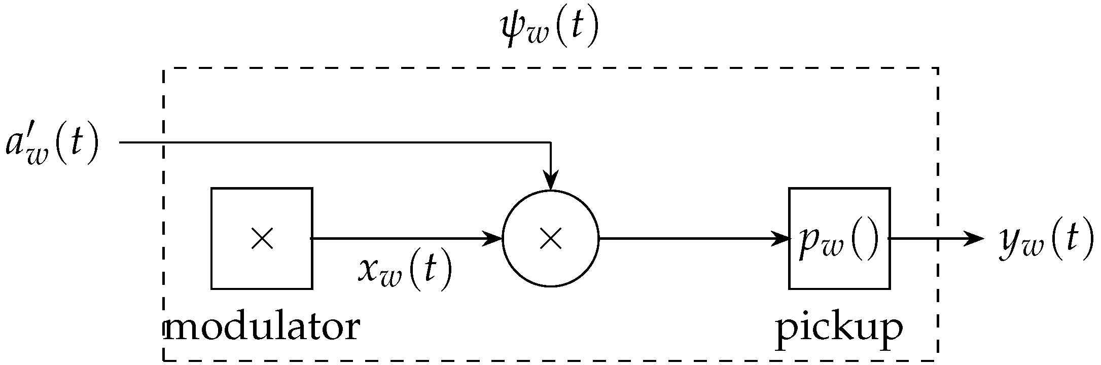
An individual tonewheel processing stage is shown in
Figure 6. Notice the slight change in architecture from the analogous
Figure 2. In
Figure 6, the pickup distortion has been moved to operate on the output rather than the raw tonewheel signal. The reason for this change is artistic—it disambiguates the effects of the memoryless pickup nonlinearities and the distortion of the tonewheel basis functions.
Finally, the output
is formed by summing all of the mode outputs:
In the rest of this section, we describe in detail how aspects of the modal processor are tuned and adapted to create the Hammondizer. Pitch processing adaptations include tuning the modes to the particular frequencies and frequency range of the Hammond organ
Section 4.1), introducing drawbar-style controls to pitch processing (
Section 4.2), adding vibrato to mode frequencies (
Section 4.3), and adding crosstalk between nearby modes to simulate crosstalk between nearby tonewheels (
Section 4.4). Distortion processing adaptations include adapting saturating nonlinearities for each mode to mimic the pickup distortion of each tonewheel (
Section 4.5) and replacing modulation sinusoids with sums of sinusoids to mimic non-sinusoidal tonewheel shapes (
Section 4.6).
4.1. Frequency Range
The first step of adapting the modal reverberator to create the Hammondizer effect is to pick the mode frequencies which specify the heterodyning and modulating sinusoids and . The unique sound of the Hammond organ is largely due to the tonewheels being tuned to the 12-tone equal tempered scale. Here we discuss how to preserve this feature in the context of the Hammondizer audio effect.
Since each mode of the modal reverberator is a narrow bandpass filter, a sufficient frequency density of modes is required to support typical wideband musical signals. In particular, unless each frequency component of the input is sufficiently close to a mode center, it may not contribute audibly to the output. For this reason, tuning the modal reverberator’s frequencies to the 12-tone equal tempered scale used by the Hammond organ heavily attenuates the frequencies “in the cracks”, producing an artificial sound (compare to composer Peter Ablinger’s “Talking Piano” [
50]).
To avoid this effect, we use many exponentially-spaced mode frequencies per semitone. Denoting the number of modes per semitone as
S, the tuning of each mode is
(cf. Equation (
2)).
S is chosen to satisfy two subjective constraints. As
S gets larger, the computational cost of the modal processor grows. As
S becomes small, the modal density decreases and produces an artificial sound. We found by experimentation that
is a good setting that balances these two constraints.
Heterodyning and modulating sinusoids at constant frequencies are given by
(cf. Equation (
18)).
The next step of adapting the modal reverberator to create the Hammondizer effect is to choose the range of mode frequencies. The range of the Hammond organ is C1 ( Hz) to F#7 ( Hz). For simplicity, we set Hz and let the modes range up seven octaves, up to Hz; these modes are indexed by a tonewheel index . These round numbers correspond very closely to the range of the Hammond organ. Forty Hz corresponds to and 5120 Hz to ; therefore, this range technically cuts off semitones from the top and bottom of the range of the Hammond organ tonewheel range. Nonetheless, it does not negatively affect the qualitative effect of the Hammondizer.
4.2. Tone Controls
The heart of the Hammondizer effect is the drawbar tone controls. As before, the drawbar settings give a column
of registrations, which drive the entries of the sparse matrix
according to
The only difference from Equation (
5) is the presence of
S to account for the multiple modes per semitone.
In the Hammondizer context, the entries in control a Hammond-style pitch shift. The structure of means that energy in a smoothed baseband signal (centered at some mode frequency ) contributes to nine different tonewheel amplitudes , according to .
4.3. Vibrato
A vibrato effect that can mimic Hammond organ vibrato is created when the frequencies of the modulating sinusoids
are varied. In this case, modulation sinusoids can be implemented with phase accumulators
Each vibrato phase signal is given by
where
is the vibrato depth in cents and
is the vibrato rate in Hz.
An early Hammond patent [
20] praises “…a musical tone containing a vibrato, that is, a cyclical shift in frequency of approximately 1.5%, at a rate of about 6 per second…” To match that design criteria, we typically choose a vibrato depth of 26 cents ≈
and a vibrato rate of 6 Hz. Of course, these can be parameterized as desired.
4.4. Crosstalk
Some aficionados point to crosstalk between tonewheels as an important part of Hammond organ sonics. We can consider that since mode filters are not “brick wall” filters, there is already a sort of crosstalk built into the Hammondizer effect.
Drawing inspiration from Pekonen et al. [
18], we can explicitly simulate leakage between adjacent tonewheels by adding another matrix multiply between
and
. This creates a new set of signals with crosstalk that includes modes one semitone away from the main modes with a crosstalk level
C:
4.5. Memoryless Pickup Nonlinearities
As detailed in [
39], distortion effects may be generated by passing a mode through a memoryless nonlinear function or by substituting a complex waveform for the modulation sinusoid waveform. Here we adapt both types of distortion to mimic aspects of the Hammond organ’s sonics and design to the Hammondizer. Note that since both kinds of distortion are applied separately to each mode, the output will contain no intermodulation products.
Drawing inspiration from the Mustonen et al.’s model of a guitar pickup [
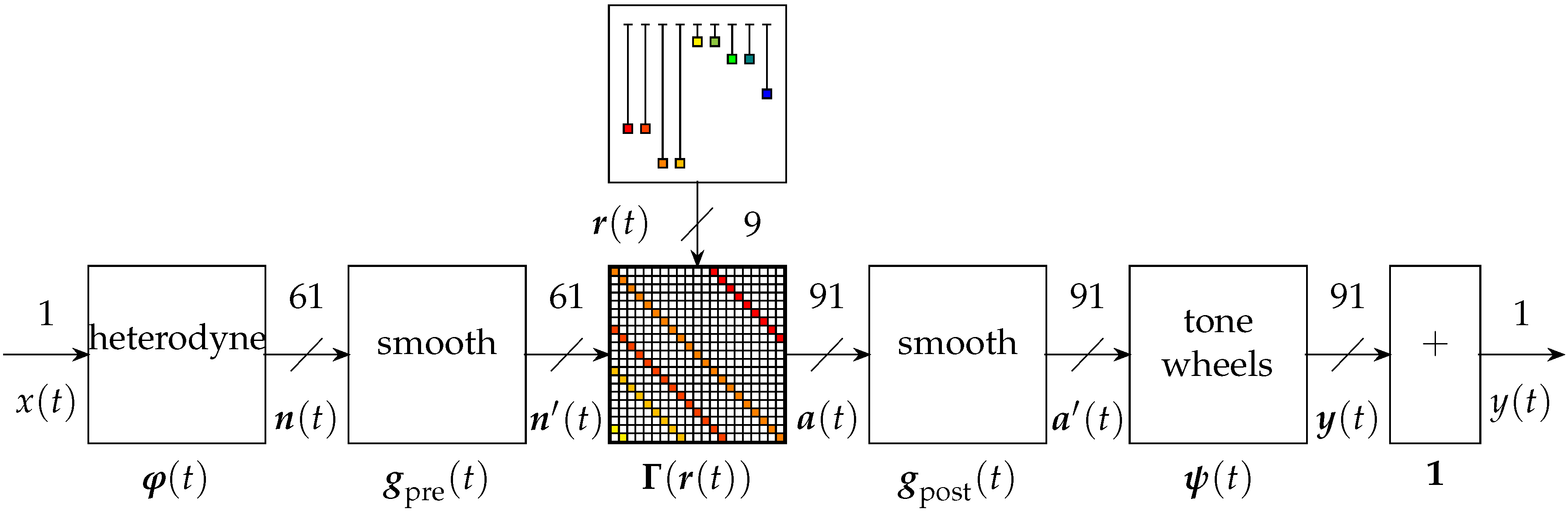
10], we propose a memoryless nonlinearity of the form
This memoryless nonlinearity is shown for values of
in
Figure 7. This has the property of maintaining unity gain around zero, but distorting signals with a large swing around zero by compressing positive signals and expanding negative signals. In this article, we will use a value of
.
Typically, memoryless nonlinearities like this will produce effects including “harmonic distortion” (new frequencies at multiples of existing frequencies) and “intermodulation products” (new frequencies at sums and differences of existing frequencies). Since this memoryless nonlinearity is applied to the output of a bandpass filter, mostly harmonic distortion will be created, since energy is concentrated at one frequency.
4.6. Tonewheel Basis Distortion
On the Hammond organ, tonewheels may not be perfectly sinusoidal. Also, the lowest octave of tonewheels are cut closer to a square wave shape than a sinusoid. This can be considered a distortion of the sinusoidal basis functions that the tonewheels represent. To approximate this distortion of the lower tonewheel basis functions, we can replace each modulating sinusoid
with a
sum of sinusoids
(cf. Equation (
10)).
Drawing inspiration from the Hammond organ, this should be done for the lowest octave of tonewheels. In practice, it can be useful to define the effect for a large range of modes.
Note that this distortion is very different in character from the saturating nonlinearities. Specifically, it has the unique feature of being amplitude-independent.
5. Results and Discussion
To demonstrate the features of the Hammondizer, we present a series of examples. Examples of the pitch processing and distortion processing Hammondizer components, operating on a pure tone input, are presented in
Section 5.1 and
Section 5.2, respectively. Examples of the full Hammondizer, applied to program material, are described in
Section 5.3. Aspects of the Hammondizer’s sonics are visible in the spectrogram and explained in the text. To understand the full effect of the Hammondizer, it is necessary to listen to it. Audio recordings (.wav file format) of all these examples are available online [
51].
For all of these examples, the Hammondizer is configured to have 1177 exponentially spaced modes, with 14 modes per semitone over the seven octave range from 40 Hz to 5120 Hz. The two columns of smoothing operations
and
are set so that the gain of each mode during the smoothing operations is set to unity.
is simply a column of ones. Except where noted, each mode is assigned a 200-ms decay time. We form
using smoothing filters which are applied twice, as suggested in [
39]. This creates impulse responses with a linear ramp onset and a 200-ms decay (e.g., [
52])—i.e., of the form
.
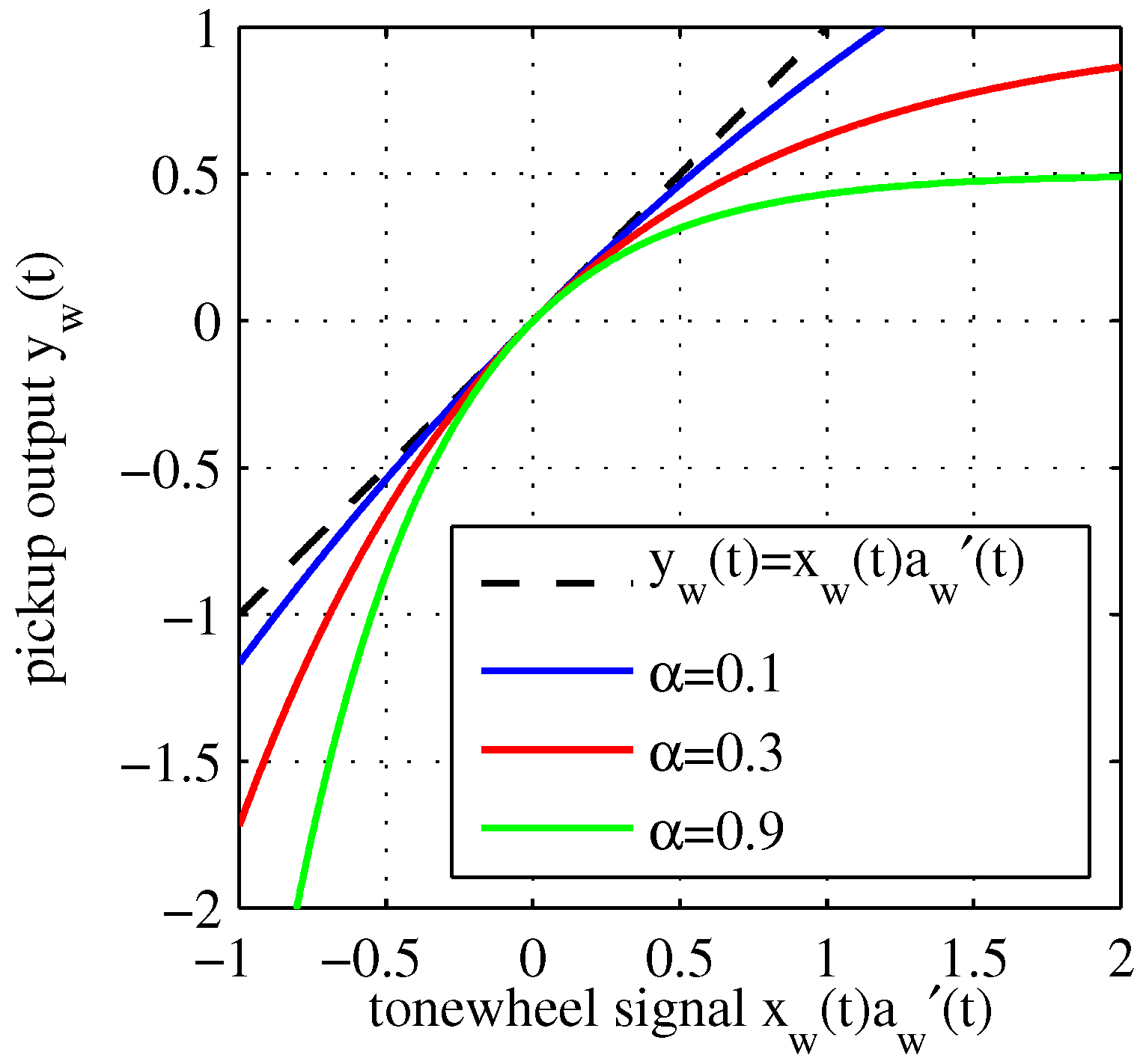
Although we have not emphasized the variation of the mode dampings and complex amplitudes in this article—focusing rather on the novel aspects of the Hammondizer—the mode dampings and complex amplitudes can be set just as in the modal reverberator [
37,
38], creating hybrid Hammond/reverb effects. effects. The different Hammond organ registrations shown in these results are given in
Figure 8 and are taken from a Hammond owner’s manual [
53] and a Keyboard Magazine article [
54]..
5.1. Pitch Processing Examples
In this section, we demonstrate the Hammondizer’s drawbar tone controls (
Figure 9), its frequency range (
Figure 10), and crosstalk and vibrato processing (
Figure 11).
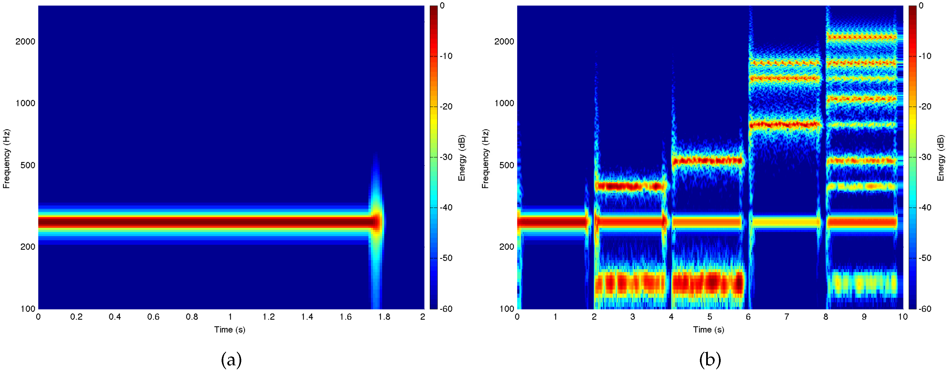
Figure 9 shows spectrograms of a pure tone input signal and versions processed with the Hammondizer. The input signal (
Figure 9a) is a
-second-long sine wave tuned to middle C (C3,
Hz). The output signal (
Figure 9b) shows five different Hammondized versions of the input signal. Each of the five versions uses a different registration; the vibrato, crosstalk, and distortion were disabled. The different Hammond organ registrations shown in these results are given in
Figure 8.
Figure 9b uses the first five registrations of
Figure 8 in order.
The C3 sine wave is tuned very close to the center frequency of mode
. Knowing that the Hammondizer uses the matrix
to drive output modes that are offset from each analysis mode by the length-9 column
(recall
Table 1 and Equation (
1)), we expect that an input consisting of a single sinusoid will in general create output signals with nine sinusoidal components (recall Equation (
11)) near modes
. However, since
is a function of the registration
, the output behavior is heavily dependent on the registration. Notice that the 008000000 registration does not affect the signal much beyond a slight lengthening due to the decay time of the modes near C3. Since each
except
is zero, only one sinusoid comes out. The second setting, “bassoon” (447000000) produces three sinusoids in response to the input sinusoid, since it has three non-zero
s. The amplitude of each sinusoid depends on its corresponding drawbar setting (recall
Table 2). The “bassoon,” “mellow-Dee,” and “shoutin’ ” registrations have non-zero first drawbar settings—notice that they produce energy an octave below C3. The “shoutin’ ” and “all out” registrations have no non-zero drawbar settings—notice that the individual sine wave of the input has driven nine sine waves in the output, and that their relative amplitudes reflect the “shoutin’ ” and “all out” registrations (668848588 and 888888888, respectively).
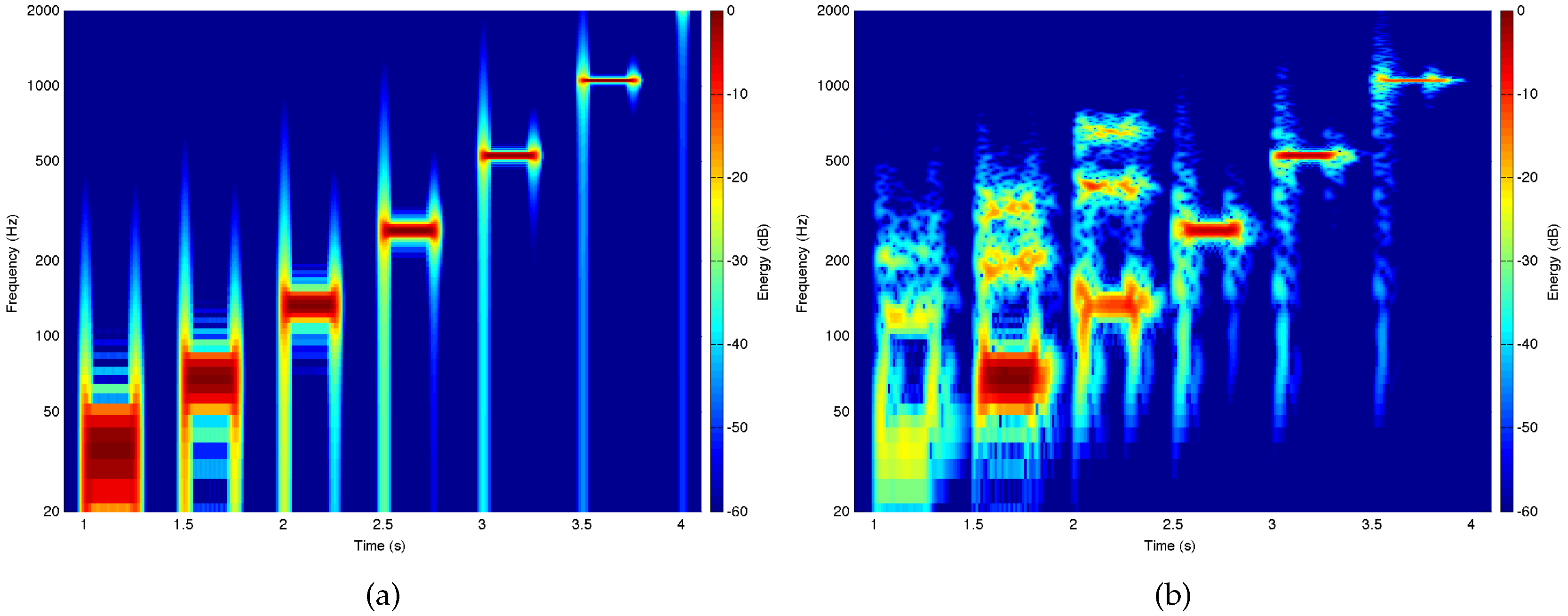
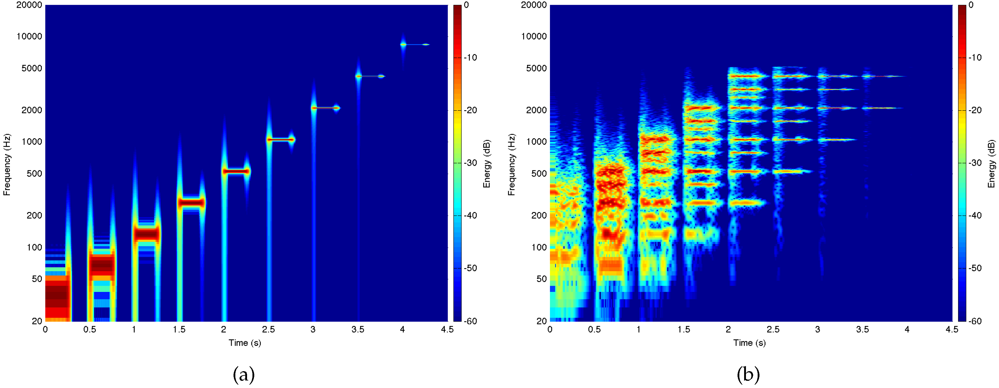
Figure 10 shows spectrograms of a sinusoidal input signal and its Hammondized response. The input signal (
Figure 10a) is a series of nine
-second-long sine waves, generated at octave intervals from C0 (
Hz) and to C8 (
Hz). The Hammondized output (
Figure 10a) used the 668848588 (“shoutin’ ”) registration, and the vibrato, crosstalk, and distortion were disabled. In a broad sense, the Hammondizer imprints the “shoutin’ ” partial structure onto the input sinusoids. Note, however, that since the Hammondizer does not have any modes outside the 40 Hz to 5120 Hz frequency range, the C0 and C8 inputs generate little output, though transients in the C0 sinusoid produce a ghostly “whoosh” sound.
The Hammondizer crosstalk and vibrato components are now explored using the pure tone input of
Figure 9a. In
Figure 11a, the effect of crosstalk is illustrated using the “clarinet” registration with vibrato and distortion disabled. Crosstalk amplitudes of
,
,
,
, and
dB are simulated. Note the increased presence of energy in adjacent notes with increased crosstalk amplitude. In
Figure 11b, the effect of vibrato is studied using a “whistle stop” (888000008) registration, with crosstalk and distortion disabled. Each output uses a 6 Hz vibrato, with (from left to right) vibrato depths of 0, 25, 50, 100, and 1200 cents, with a depth of 25 cents being typical for a Hammond tonewheel organ. As expected, there is a sinusoidal variation in the output frequency of each partial.
5.2. Distortion Processing Examples
Figure 12 shows an input signal spectrogram (
Figure 12a) and a Hammondized version showing the tonewheel shape distortion (
Figure 12b). The input signal is the collection of sinusoids C0 through C5. This is applied to the Hammondizer set to a fundamental-only registration (008000000), with vibrato and distortion disabled. As described above, the lowest two octaves of tonewheels are given 3rd and 5th harmonics. Notice how C0, C1, and C2 produce pronounced 3rd and 5th harmonics even though the registration is 008000000, but that C3–C5 don’t generate harmonics.
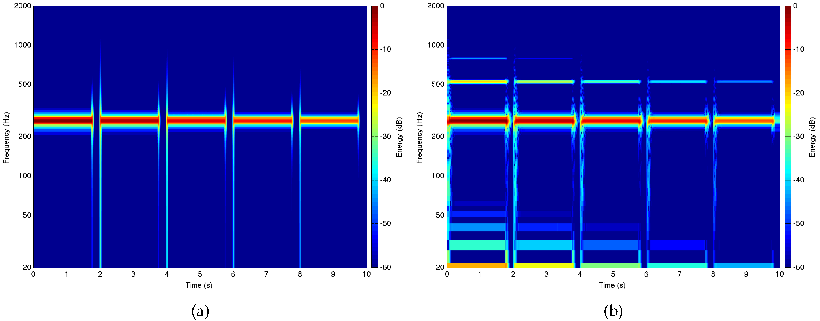
Figure 13 shows spectrograms of an input signal and its Hammondized version.
Figure 13a shows the input signal: five
-second-long sinusoidal bursts, all tuned to C3. From left to right, the input sinusoid amplitudes are 0,
,
,
, and
dB. Notice in the output (
Figure 13b) that the degree of distortion decreases as the amplitude decreases, as is typical of saturating memoryless nonlinearities.
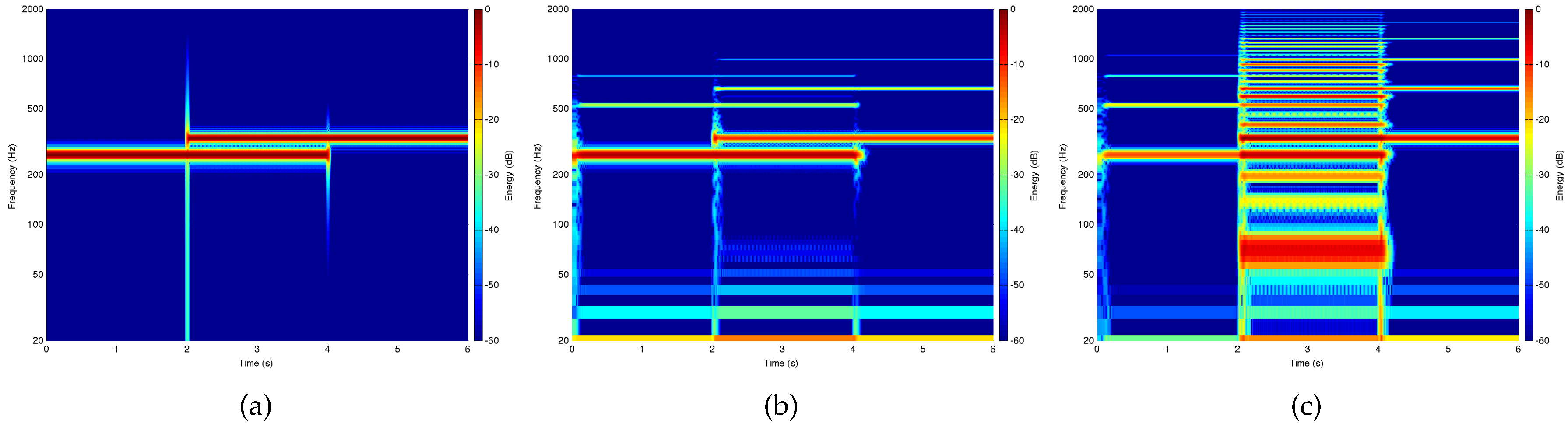
Recall that the Hammond distortion is generated separately on each key, and accordingly there is no intermodulation distortion. To demonstrate this and to test the presence of intermodulation distortion in our Hammondizer process, we use a signal having C3 and E3 notes which appear both individually and overlapped—see
Figure 14.
Figure 14b shows the Hammondized result. Notice that there is little to no intermodulation distortion in the output; the response to the combination of C3 and E3 is very nearly equal to the sum of the response to C3 and the response to E3.
Figure 14c shows the result of a modified algorithm
in which the hundreds of individual mode pickup distortions are replaced by a single pickup distortion that operates on the sum of all modes. (cf. Equations (
24) and (
25)). This more typical approach to implementing distortion produces heavy intermodulation distortion. This sort of intermodulation distortion can be considered unpleasant; its absence can be considered a unique feature of the Hammondizer.
5.3. Full Examples
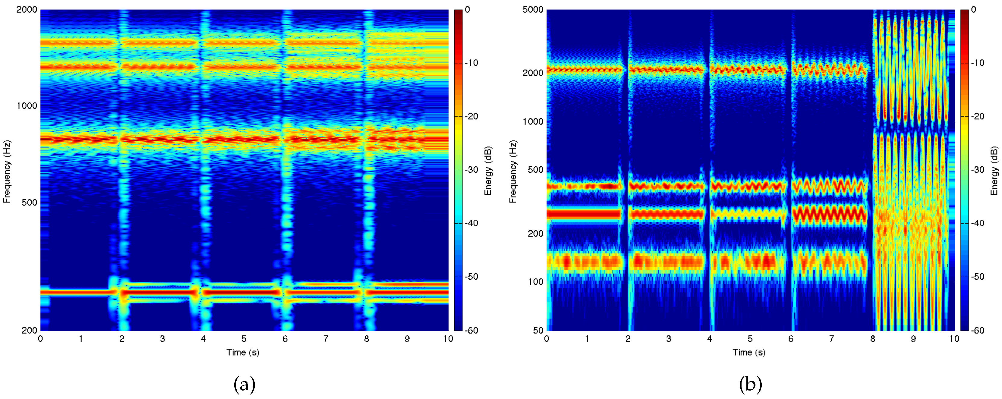
In this section, we present examples of the full Hammondizer processing program material, a guitar (
Figure 15) and a violoncello (
Figure 16).
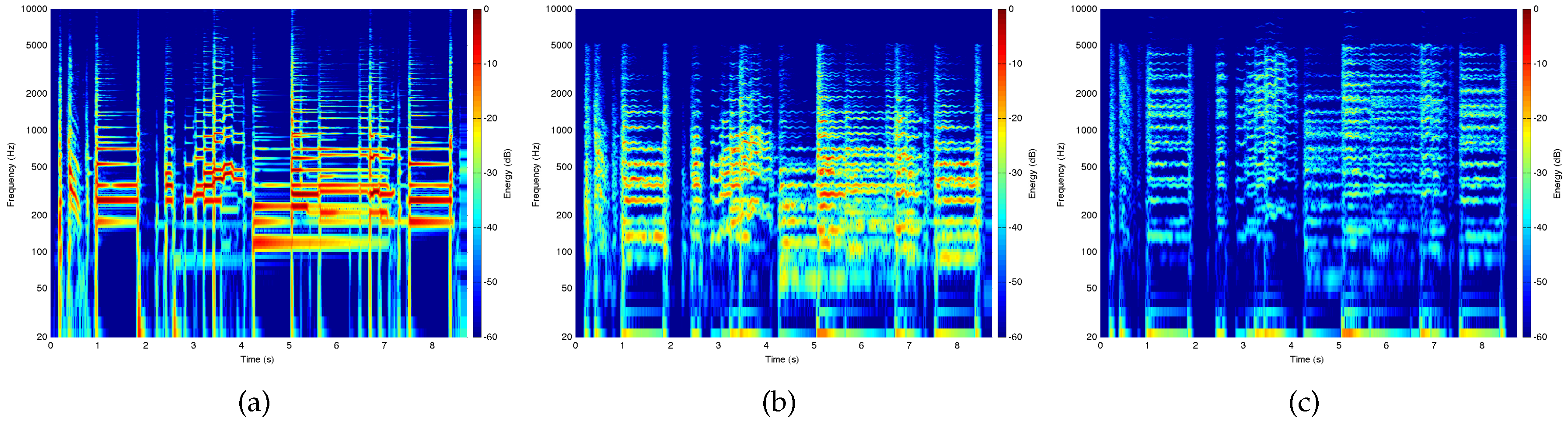
Figure 15a shows a blues guitar lick, and two Hammondized versions, with a “Jimmy Smith” (888800000) registration in
Figure 15b and an “all out” (888800000) registration in
Figure 15c. Notice that the relatively full-range input of the guitar is mostly restricted to below 5120 Hz in the Hammondized examples. Especially from 1–2 s, the vibrato is visible. In the “all out” registration, some pickup distortion is visible above the 5120-Hz tonewheel limit.
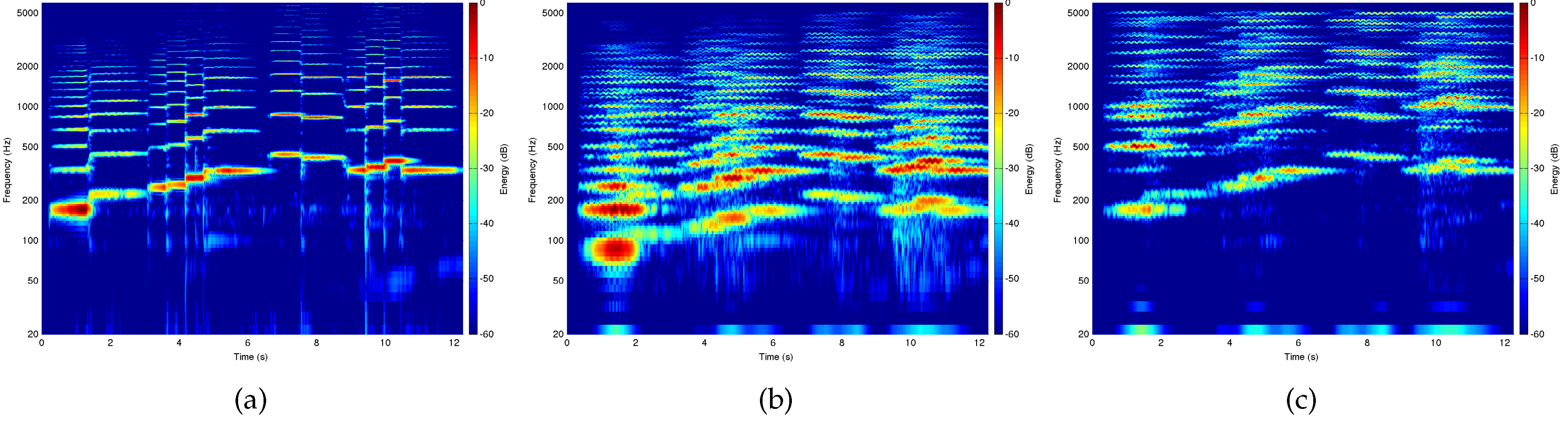
Figure 16a shows a melody “El Cant dels Ocells” played on the violoncello, and two Hammondized versions, with a “bassoon” (447000000) registration in
Figure 16b and a “clarinet” (006070540) registration in
Figure 16c.
6. Conclusions
In this article, we’ve described a novel class of audio effects—the Hammondizer—that imprints the sonics of the Hammond tonewheel organ on any audio signal. The Hammondizer extends the recently-introduced modal processor approach to artificial reverberation and effects processing. We close with comments on two extensions to the Hammondizer audio effect.
We’ve discussed parameterizations of each aspect of the Hammondizer which are chosen to closely mimic the sonics of the Hammond organ. For example, the mode frequency range of the Hammondizer is chosen to match the range of tonewheel tunings on the Hammond organ, and the the vibrato rate and depth are chosen to mimic a standard Hammond organ vibrato tone. In closing, we wish to mention that these parameterizations can be extended to loosen the connection to the Hammond organ but widen the range of applicability of the Hammondizer. For instance, the mode frequencies can be tuned across the entire audio range (≈20–20000 Hz) rather than being limited to 40–5120 Hz. In this context, some of the connection with the Hammond organ is relaxed, but the drawbar controls still give a powerful and unique interface for pitch shift in a reverberant context.
Although the Hammondizer is designed to process complex program material as a digital audio effect, it is possible to configure the Hammondizer so that it will act somewhat like a direct Hammond organ emulation. This can be done by driving the Hammondizer with only sinusoids (e.g., a keyboard set to a sinusoid tone) which act as control signals, effectively driving
directly. This is particularly effective using short mode dampings (as in this article). An example is given alongside the other audio online [
51].


