Wavelet Packet Decomposition to Characterize Injection Molding Tool Damage ^†

Abstract

This paper presents measurements of acoustic emission (AE) signals during the injection molding of polypropylene with new and damaged mold. The damaged injection mold has cracks induced by laser surface heat treatment. Standard test specimens were injection molded, commonly used for examining the shrinkage behavior of various thermoplastic materials. The measured AE burst signals during injection molding cycle are presented. For injection molding tool integrity prediction, different AE burst signals’ descriptors are defined. To lower computational complexity and increase performance, the feature selection method was implemented to define a feature subset in an appropriate multidimensional space to characterize the integrity of the injection molding tool and the injection molding process steps. The feature subset was used for neural network pattern recognition of AE signals during the full time of the injection molding cycle. The results confirm that acoustic emission measurement during injection molding of polymer materials is a promising technique for characterizing the integrity of molds with respect to damage, even with resonant sensors.

1. Introduction

Injection molding is still regarded as one of the most important and very popular manufacturing process because of its simple operation steps. A typical production cycle begins with the mold closing, followed by the injection of melt into the mold cavity. Once the cavity is filled, holding (packing) pressure is applied to compensate for the material shrinkage. In the next step, the screw turns, feeding the material for the next shot to the screw tip. This causes the screw to retract as the next cycle is almost ready. Once the molded part is sufficiently cooled, the mold opens and the part is finally ejected.

Chen and Turng [1] defined three categories of variables that characterize the hierarchy and dependencies of an injection-molding control system. The first-level variables are defined as machine variables and include barrel temperatures in several zones, pressure, sequence and motion, etc. The second-level variables are process-dependent variables that include melt temperature in the nozzle, runner and mold cavity, melt pressure in the nozzle and cavity, melt-front advancement, maximum shear stress, and rate of heat dissipation and cooling. The third level incorporates quality measures such as part weight and thickness, shrinkage and warpage, etc. Current research mostly deals with the control tasks at the first two levels. For quality control purposes, this is often achieved indirectly through online dynamic process control or offline statistical process control (SPC). The majority of commercially available in-mold sensors for monitoring second level variables are pressure and temperature sensors.

Zhang et al. [2] applied a mechanical wireless data transmission technique using ultrasonic waves as the information carrier for online injection mold cavity pressure measurements. Ultrasonic transmitters with specific frequency characteristics were designed, modeled, simulated, and prototyped for pressure data retrieval from an enclosed machine environment. Lijuan Zhao et al. [3] developed an ultrasonic monitoring technique using a high-temperature ultrasonic transducer for real-time diagnostics in polymer processing and tracking of morphologic changes in injection molding processing.

The location and propagation of a crack in the metal can be detected using the acoustic emission technique, as already reported by many researchers. The major AE signal sources detected by NDT are crack growth and plastic deformation of the steel [4]. Acoustic emission (AE) as transient elastic waves has drawn a great deal of attention because of its applicability to online surveillance and capability to acquire data with high sensitivity [5,6,7]. Cao et al. [8] investigated acoustic emission (AE) signals during four-point bending fatigue crack propagation in the base metal and weld of −16 Mn steel. In the first stage of fatigue damage process micro-crack initiation was a dominant AE source. During stable crack extension (intermediate stage), stacking and slipping of dislocations ahead of the crack tip are sources of AE signals. During unstable crack extension (final stage) shearing of ligaments and connectivity between dimples are AE sources. Input parameters of their neural network model are based on burst energy, peak amplitude, duration, and counts. Mukhopadhyay, et al. [9] investigated AE signals during fracture toughness tests of steel CT specimens. The AE generated during fracture toughness tests has been attributed to the plastic zone formation at the crack tip and initiation and/or extension of crack. They measured burst peak amplitude and RA value and used the differentiation of the AE burst signals’ RMS voltage, count, and energy with respect to time by taking the average of the slopes of adjacent data points to evaluate fracture toughness. Drummond et al. [10] investigated enhancement of proof and fatigue testing procedures for wire ropes by incorporating AE signals. They suggested that to differentiate between signals from wire breaks and other sources, the most effective AE signal discriminators are peak amplitude and (cumulative) burst energy. Also, the rope’s condition can be ascertained without the necessity of continuous monitoring and the AE emission is indicative of the level of damage. Ki-Bok Kim et al. [11] analyzed fatigue crack growth in standard CT specimens with a hydraulic loading machine. The objective of their research was the development of a neural network-based model for the prediction of stress intensity factor as a function of five basic AE parameters (ring down count, rise time, energy, event duration, peak amplitude). Their research proved that AE energy increases gradually as the number of fatigue cycles increases. Change in the AE energy with the fatigue cycle number could be one of the effective parameters to estimate the activity of the crack propagation and the stress intensity factor.

The AE method provides a huge potential for extensive in situ failure analysis of materials, since it provides information on sub-macroscopic failure phenomena as well as on the overall damage accumulation [12]. Generated AE signal contains useful information on the damage mechanism. One of the main issues of AE is to discriminate the different damage mechanisms from the detected AE signals. Each signal can be associated to a pattern composed of multiple relevant descriptors [13,14,15,16]. Then the patterns can be divided into clusters representative of damage mechanisms according to their similarity by the use of multivariable data analyses based on pattern recognition algorithms [17].

Piezoelectric sensors can measure ultrasound with a sensitivity of about 1 V/nm as displacement sensors and a few V/(mm/s) as velocity sensors. The dynamic amplitude range of piezoelectric sensors is around 120 dB. Another useful property when measuring ultrasound is that they measure only dynamic events and so automatically compensate for low-frequency motion of measuring objects that are caused by environmental vibrations. This intrinsic low-frequency cutoff is a consequence of the leakage of the accumulated charge. This acts as a high-pass filter that determines the low-frequency cutoff (compensational bandwidth) through a time constant given by the capacitance and resistance of the device [18]. Additionally, piezoelectric sensors are also insensitive to electromagnetic fields and radiation, enabling measurements under harsh conditions.

Correlation of basic AE burst signal parameters (peak amplitude, energy, RMS value, RA value, burst count, etc.) and crack propagation in steel are well described in the literature. The detection of damage in molds during the injection molding process is a topic that has not gained sufficient coverage in the literature, although injection molding is one of the most widely used production process. In this paper we present the possibility of damage detection and process steps based on time domain, frequency domain variables, and wavelet packet transform descriptors of AE bursts.

The first steps towards characterizing injection molding tool damage and process phases are the determination and calculation of AE descriptors for acquired AE bursts (Section 3.1). These descriptors are stacked to form a feature (measurement) vector Z. The next step is unsupervised fuzzy C means (FCM) clustering to separate the bursts characteristic for damage (cluster 5) of injection molding tool from the AE bursts characteristic for injection of the melt and holding stage of the injection molding process (Section 3.2). AE bursts of cluster 5 can be acquired only during injection molding with a damaged tool. Next we introduced a feature selection method to select the 10-dimensional feature subset from the 73-dimensional feature vector to improve suitability for classification (Section 3.3). Next, the feature subset was used for neural network pattern recognition of AE signals during the full time of the injection molding cycle (Section 3.4). At the end of the paper we present a classification of all input vectors and an evaluation of the proposed method to characterize injection molding tool damage and process phases.

2. Experimental Section

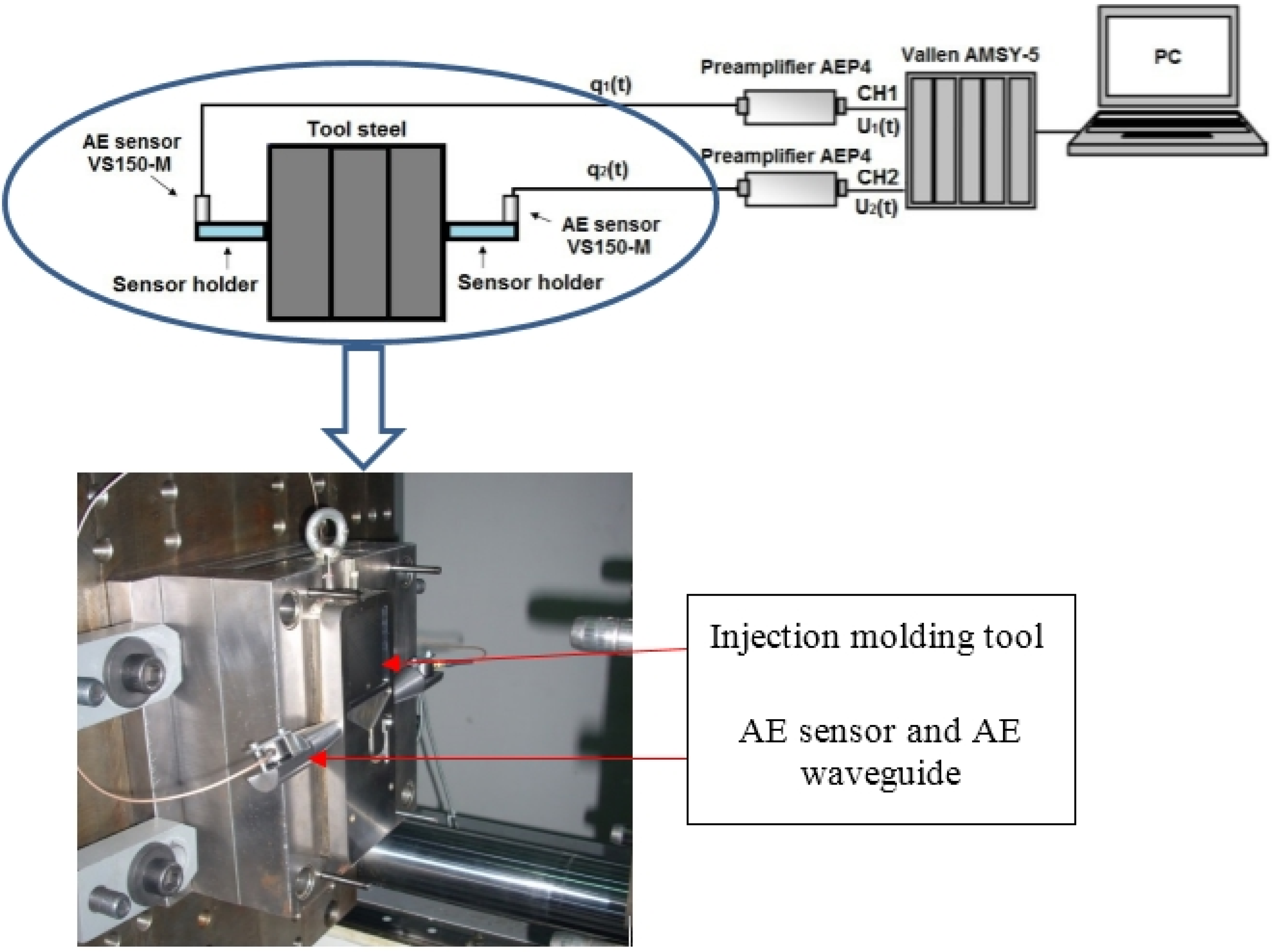
Acoustic emission signals were captured during the production cycle of standard test specimens, designed for shrinkage evaluation of various plastic materials. We used an injection molding tool (TECOS, Celje, Slovenia) with one cavity for production of standard D2 ISO test specimens with square dimensions of 60 × 60 × 2 mm³, which can be used for a variety of tests according to ISO 294-3. The injection molding tool is made of OCR12VN steel. A polypropylene material isofil H40 C2 F NAT manufactured by Sirmax (Cittadella, Italy), mainly used in the automotive industry, was employed. A Vallen-Systeme GmbH acoustic emission measurement system AMSY-5 (Vallen-Systeme GmbH, Icking, Germany) was used to capture and analyze the AE signals at 5 MHz sampling frequency. Two piezoelectric AE sensors VS150-M with a measuring range between 100 and 450 kHz and resonance at 150 kHz were mounted on both sides of the tool via waveguides, as shown in Figure 1. These sensors are widely used in AE testing and monitoring and are low cost. The sensor also covers frequencies characteristic for AE signals generated during plastic deformation and fatigue [19]. We used an 18-kHz high pass filter (Vallen-Systeme GmbH, Icking, Germany). AE waveguides protect the sensors against the high surface temperature of injection molds during the production cycle, possible fumes exhaled out of the mold, and damage in case operator intervention is needed to help remove the specimen. The length of the waveguide is determined based on experience to protect sensors against the aforementioned hazards. PZT sensors were connected to the AMSY-5 measurement system via two AEP4 preamplifiers (Vallen-Systeme GmbH, Icking, Germany) with a fixed gain of 40 dB. The amplitude threshold was set at 40 dB. Experiments were conducted on a hydraulic injection molding machine KM 80 CX-SP 380 (KraussMaffei Group, Munich, Germany), for a broad spectrum of injection molding process parameters.

Figure 1. Experimental setup for AE monitoring during the injection molding process.

Figure 1. Experimental setup for AE monitoring during the injection molding process.

3. Results and Discussion

AE monitoring is a very promising method for the detection of injection mold defects. Namely, the rapid increase of mold pressure during the filling and holding stages of the injection molding process can trigger defects (acoustic emission sources) in the tool steel. Acoustic emission testing can detect dynamic processes associated with the degradation of structural integrity.

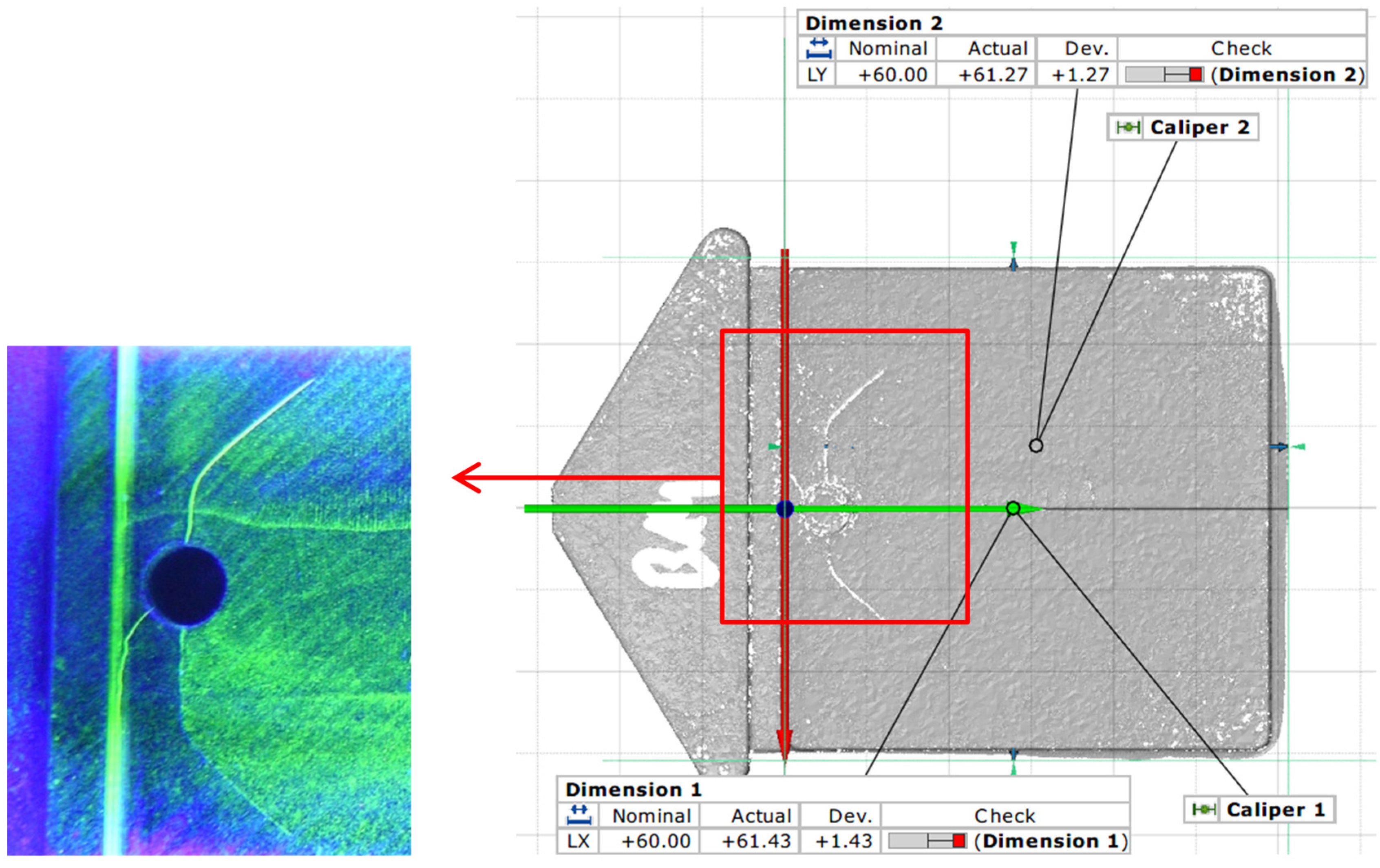
Figure 2. Cracks in the injection molding tool and accompanying PP specimen.

Figure 2. Cracks in the injection molding tool and accompanying PP specimen.

Experiments were conducted using a new injection mold tool and a damaged tool, respectively. Surface cracks were generated by successive local laser surface hardening of the tool steel. Both tools were tested using magnetic particle testing with fluorescent magnetic suspension. The cracks detected on the damaged tool are presented in Figure 2. After 24 h, the standard injection-molded polypropylene test specimens were scanned with an optical ATOS II SO 3D-digitizer. The ATOS II SO 3D digitizer is based on the triangulation principle whereby a sensor unit first projects different fringe patterns onto the scanned object’s surface, which is then recorded by two cameras. Each measurement generates up to 4 million data points. In order to digitize a complete object, several individual measurements from different angles are required. The cracks on the damaged tool are also reflected on the surface of injection molded specimens. Shape deviations (Figure 2) in two dimensions from the ideal shape are stated in mm.

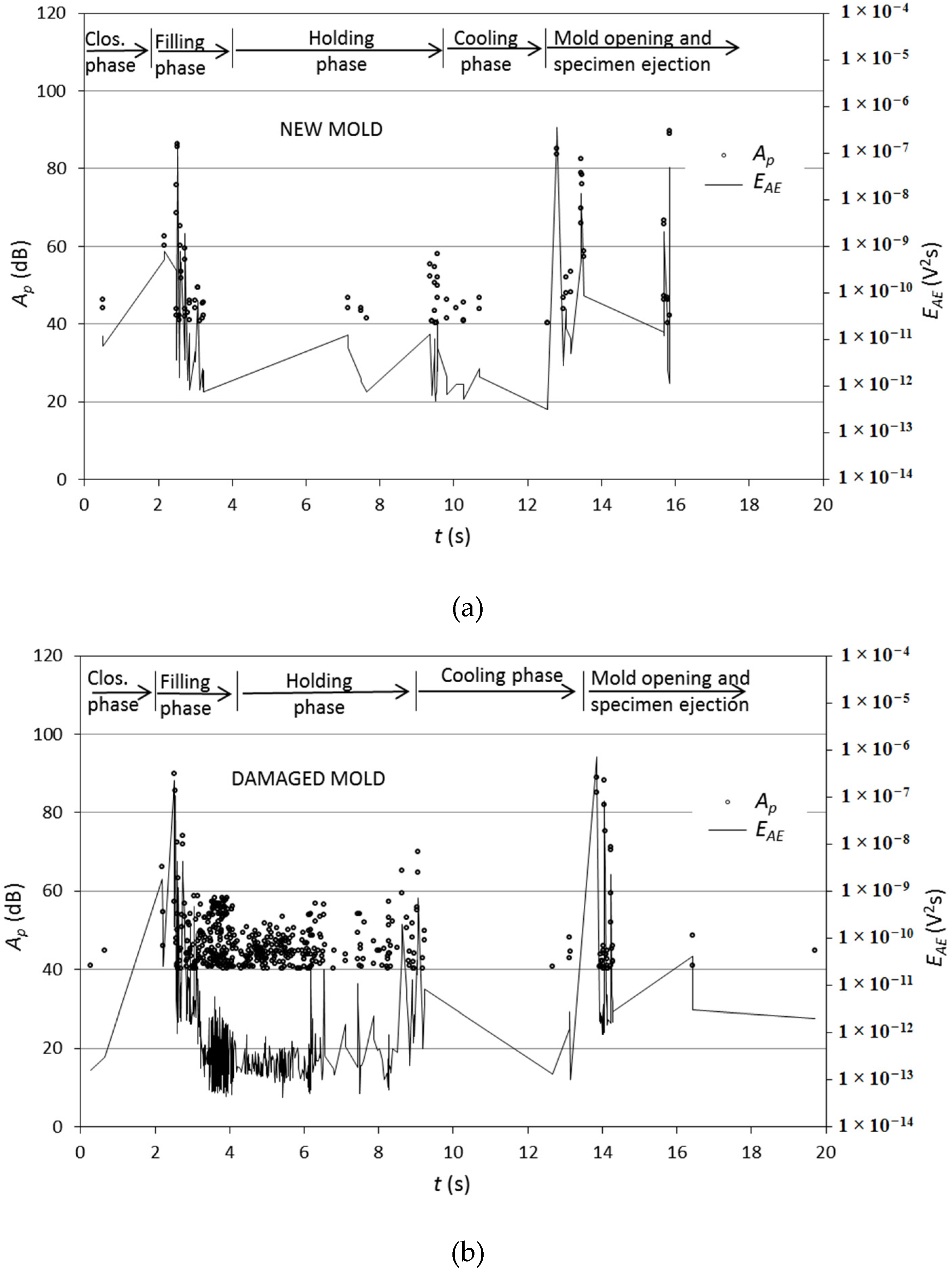
Figure 3. AE bursts’ amplitude and energy during injection molding with (a) a new mold and a (b) damaged mold.

Figure 3. AE bursts’ amplitude and energy during injection molding with (a) a new mold and a (b) damaged mold.

Figure 3 shows peak amplitudes and energy of AE bursts during the manufacturing of test specimens produced in the new and damaged mold, respectively. Absence of damage in the new tool offers us the opportunity of classifying measured AE bursts as process-orientated signals. On the other hand, the presence of a damaged area in the injection molding tool causes a considerable increase in the number of AE bursts detected during the filling and holding phases, above all in an amplitude range between 40 and 60 dB. Consequently, we can ascribe the additional AE bursts measured during the filling and holding phase to active AE sources from injection mold defects. A rapid increase in mold pressure during the filling phase could stimulate plastic zone formation, stacking, and slipping of dislocations ahead of the crack tip and crack extension [8,9] in the tool steel. Plastic deformations in the vicinity of the crack in the steel, mostly related to sliding dislocations, and crack growth cause distinctive AE bursts [20]. We connected AE signals with propagation of damage in the insert but this incorporates, based on the research of other authors, several physical phenomena that we described in the article as possible sources. The injection molding cycle ends after 16 s when the part is ejected out of the mold.

3.1. AE Burst Descriptors

Measured AE bursts are used for derivation of AE descriptors. These descriptors are stacked to form a feature (measurement) vector Z = (z₁,z₂,…,z₇₃), representing acquired AE bursts during different phases of injection molding process. The union of 704 feature vectors, in this paper, composes feature space. AE burst is extracted from acquired AE waveform based on defined rearm time; in our research this was 0.46 ms. An AE burst is over when the rearm time elapses due to the absence of threshold crossings.

Calculated time domain descriptors based on acquired AE bursts are: peak amplitude value A_p, duration d, rise time Rt, and RA value. RA value is the ratio of rise time and amplitude of AE burst [15]. We calculated frequency domain descriptors. The P_L parameter characterizes the lower part of the power spectrum of each AE burst (a = 90 kHz, b = 190 kHz). Parameter P_H characterizes the higher part of the power spectrum (a = 250 kHz, b = 350 kHz), and parameter P_S covers all power spectrum frequencies (a = 50 kHz, b = 550 kHz). The parameters P_L, P_H, and P_S carry information about the energies at various frequencies in a sensor’s frequency spectrum:

$$g_i=\frac{y\overline{yi}}{m}$$

(1)

$$m=\max \left(Y·\overline{Y}\right)$$

(2)

$$P_L={\sum }_{a=90}^{b=190}{g}_i$$

(3)

Y = (y₁,y₂,…,y_n) represents the vector of the discrete Fourier transform using FFT.

We introduced the kurtosis and skewness parameters describing the amplitude distribution of recorded AE burst. Kurtosis is a measure of the “peakedness” of the probability distribution for a real-valued random variable. In our case we calculated the kurtosis of measured AE burst amplitude values. Kurtosis was used in our research to characterize infrequent extreme deviations of amplitude values in AE burst as:

$$K=\frac{E{(a_i-\overline{a})}^4}{s^4}$$

(4)

where s is a sample standard deviation, a_i is an amplitude value.

Skewness S is defined as a third central moment of amplitude values in AE burst about its mean value. Skewness is in our research was used as a measure of asymmetry about the mean amplitude value of AE burst and is defined as:

$$S=\frac{E{(a_i-\overline{a})}^3}{s^3}$$

(5)

Wavelet Packet Analysis Descriptors

Wavelet analysis overcomes the pitfalls of Fourier methods and is suitable for processing AE signals during injection molding. The wavelet packet analysis is a subtler multiresolution analysis, which decomposes signal into multi-levels in the whole frequency band [21]. The detail of the signal is decomposed as well, so the frequency resolution is improved [22]. The wavelet packets include information on signals in different time windows at different resolutions. Each packet corresponds to some frequency band. Some packets contain important information while others are relatively unimportant.

Wavelet packet transform of energy limited signal X(t) can be computed using the algorithm below:

$$P_0^1\left(t\right)=X\left(t\right)$$

(6)

$$P_j^{2i-1}\left(t\right)=H{P}_{j-1}^i\left(t\right)$$

(7)

$$P_j^{2i}\left(t\right)=G{P}_{j-1}^i\left(t\right)$$

(8)

where $P_j^i\left(t\right)$ is the i^th packet on j^th resolution, with time parameter t = 1,2,…,2^J−j, i = 1,2,…,2^j, j = 1,2,…,J, J = log₂N. Operators H and G are convolution sum defined as:

$$H\{·\}={\displaystyle \sum }_{k}h\left(k-2t\right)$$

(9)

$$G\{·\}={\displaystyle \sum }_{k}g\left(k-2t\right)$$

(10)

where h(t) and g(t) are a pair of quadrature mirror filters and a time parameter t is taken as a series of integers k (t → k = 1, 2, …).

The energy of each wavelet packet is defined as:

$$E_j^i= {\displaystyle \sum }_{t=1}^{2^{J-j}}{(P_j^i\left(t\right))}^2$$

(11)

The energy of wavelet packets on selected resolution j is processed by normalization, and normalization value of each packet is

$$R_j^i=E_j^i/{\displaystyle \sum }_{i=1}^{2^j}{E}_j^i$$

(12)

Based on described AE signal descriptors, we have set the feature vector as Z = (P_H, P_L/P_H, P_L/P_S, K, S, A_p, Rt, RA, d, $R_5^1$, $R_5^2$, …, $R_5^{32}$, $E_5^1$, $E_5^2$, …, $E_5^{32}$).

3.2. Unsupervised Fuzzy C Means Clustering

We used unsupervised fuzzy C means clustering (FCM) for classification of feature vectors Z_j (j = 1, n) into D = 2 clusters. FCM clustering was found to be an effective algorithm for separating AE patterns composed of multiple features extracted from the AE waveforms [17,23]. Cluster 2 represents AE bursts during injection of the melt, cluster 3 represents process-orientated AE bursts during the holding stage, and cluster 5 bursts indicate damage during the injection and holding stages of the injection molding process. We used AE bursts measured during the injection molding process with a damaged tool, since we can also acquire AE signals representing cluster 5. We used fuzzy partitioning to connect feature vector Z_j (j = 1, n) to cluster ω_i (i = 1, D) with different membership grades u_i(Z_j) between 0 and 1.

With FCM we find cluster centers V = [K₁|K₂] that minimize the function J:

$$J\left(U,V\right)={\displaystyle \sum }_{j=1}^n{{\displaystyle \sum }}_{i=1}^D{\left[u_i\left(Z_j\right)\right]}^f{d}_e^2\left(Z_j,K_i\right)$$

(13)

U is the membership matrix with D lines and n columns with elements u_i(Z_j) representing the membership value of the j^th feature vector Z_j to the cluster ω_i with a condition:

$${\sum }_{1=1}^D{u}_i\left(Z_j\right)=1$$

(14)

f is a scalar representing the fuzzy degree. The square of Euclidian distance d_e between the feature vector and the cluster is:

d_e²(Z_j,K_i) = (Z_j-K_i)´(Z_j-K_i)

(15)

The algorithm of FCM has the following steps [17]:

(1)

the membership matrix U is randomly initialized with values between 0 and 1 that represent the membership values u_i(Z_j) of the n feature vectors Z_j (j = 1, n) to each cluster ω_i (i = 1, D).

(2)

The new cluster centers K_i are calculated according to:

$$K_i=\frac{{\sum }_{j=1}^n{\left[u_i\left(x_j\right)\right]}^f{x}_j}{{\sum }_{j=1}^n{\left[u_i\left(x_j\right)\right]}^f}$$

(16)

(3)

The membership matrix U is updated such that:

$$u_i\left({\mathrm{Z}}_j\right)={\left[{\displaystyle \sum }_{k=1}^D{\left(\frac{d\left(Z_j,K_i\right)}{d\left(Z_j,K_k\right)}\right)}^{2/\left(f-1\right)}\right]}^{-1}$$

(17)

Steps 2 and 3 are iterated until the improvement over the previous iteration is below a threshold θ where β are the iteration steps:

‖U^β−U^β−1‖ < θ, 0 <θ < 1

(18)

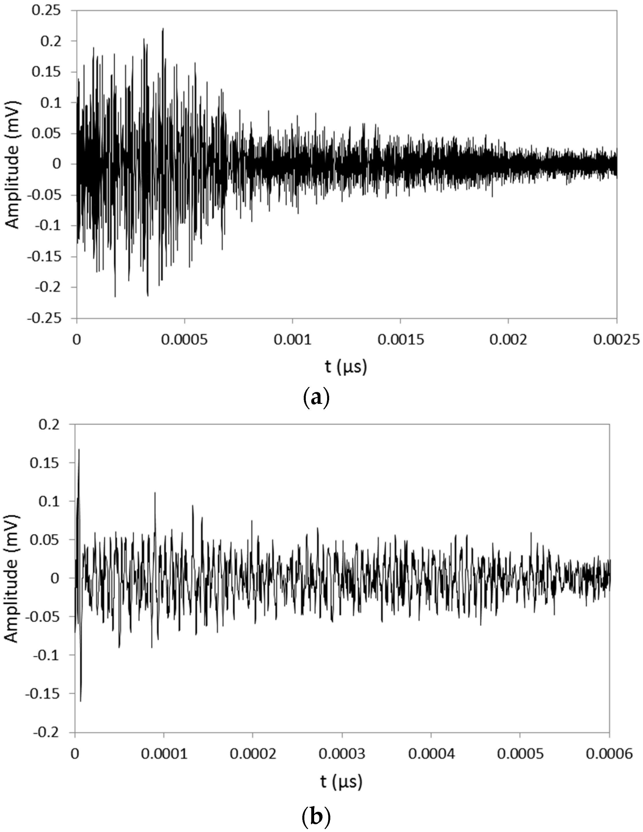
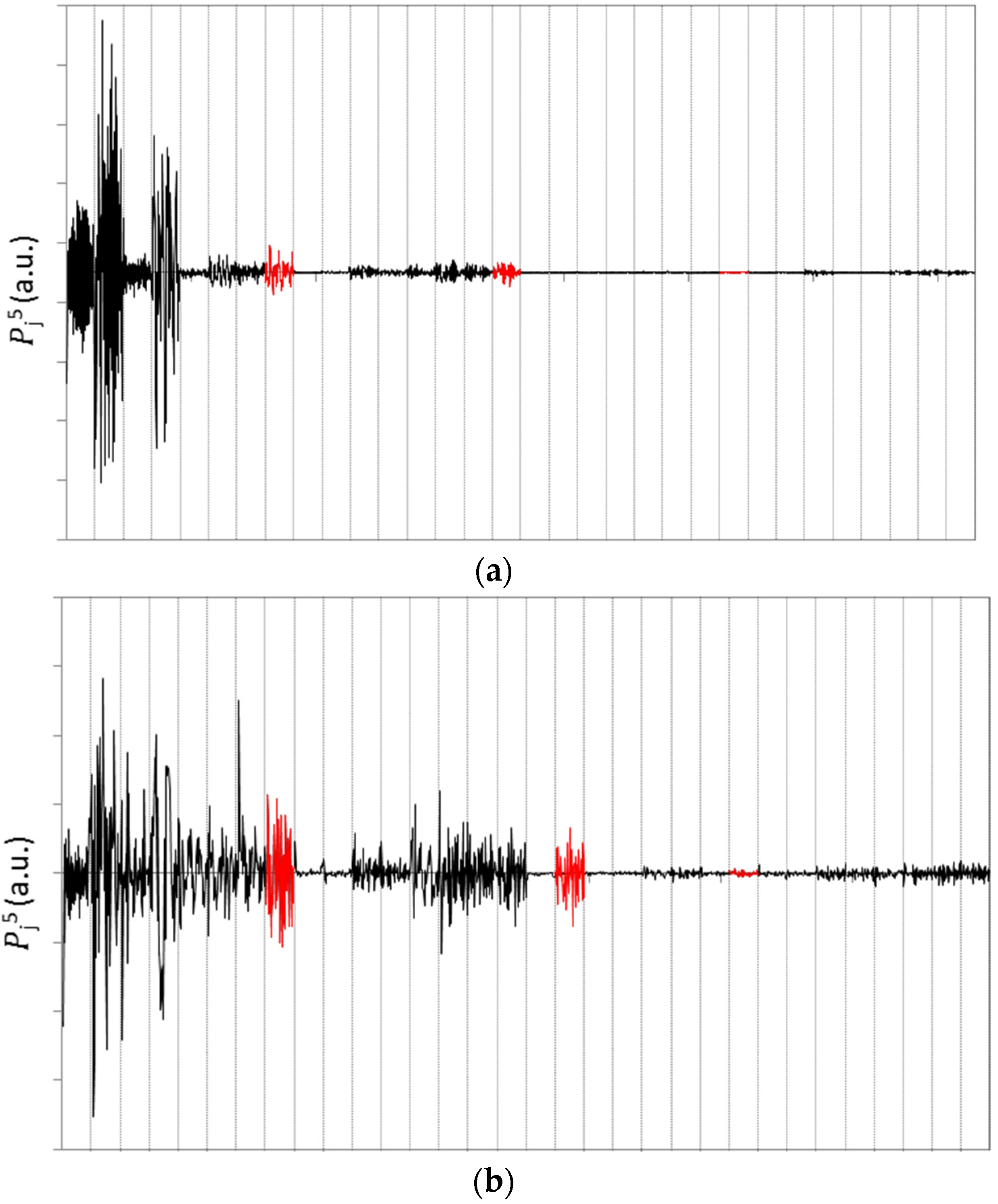
Figure 4 shows examples of signals designated as process-orientated AE burst (cluster 3) and AE burst indicating damage (cluster 5). Figure 5 shows wavelet packet coefficients associated with all 32 nodes on 5th resolution of the wavelet packet tree for signals represented on Figure 4. With a red color, coefficients associated with nodes 8, 16, and 24 on 5th resolution are emphasized.

Figure 4. Signals designated as process-orientated AE burst (a) and AE burst indicating damage (b).

Figure 4. Signals designated as process-orientated AE burst (a) and AE burst indicating damage (b).

Figure 5. Wavelet packet coefficients associated with all the nodes on 5th resolution of the wavelet packet tree for above process-orientated AE burst (a) and AE burst indicating damage (b).

Figure 5. Wavelet packet coefficients associated with all the nodes on 5th resolution of the wavelet packet tree for above process-orientated AE burst (a) and AE burst indicating damage (b).

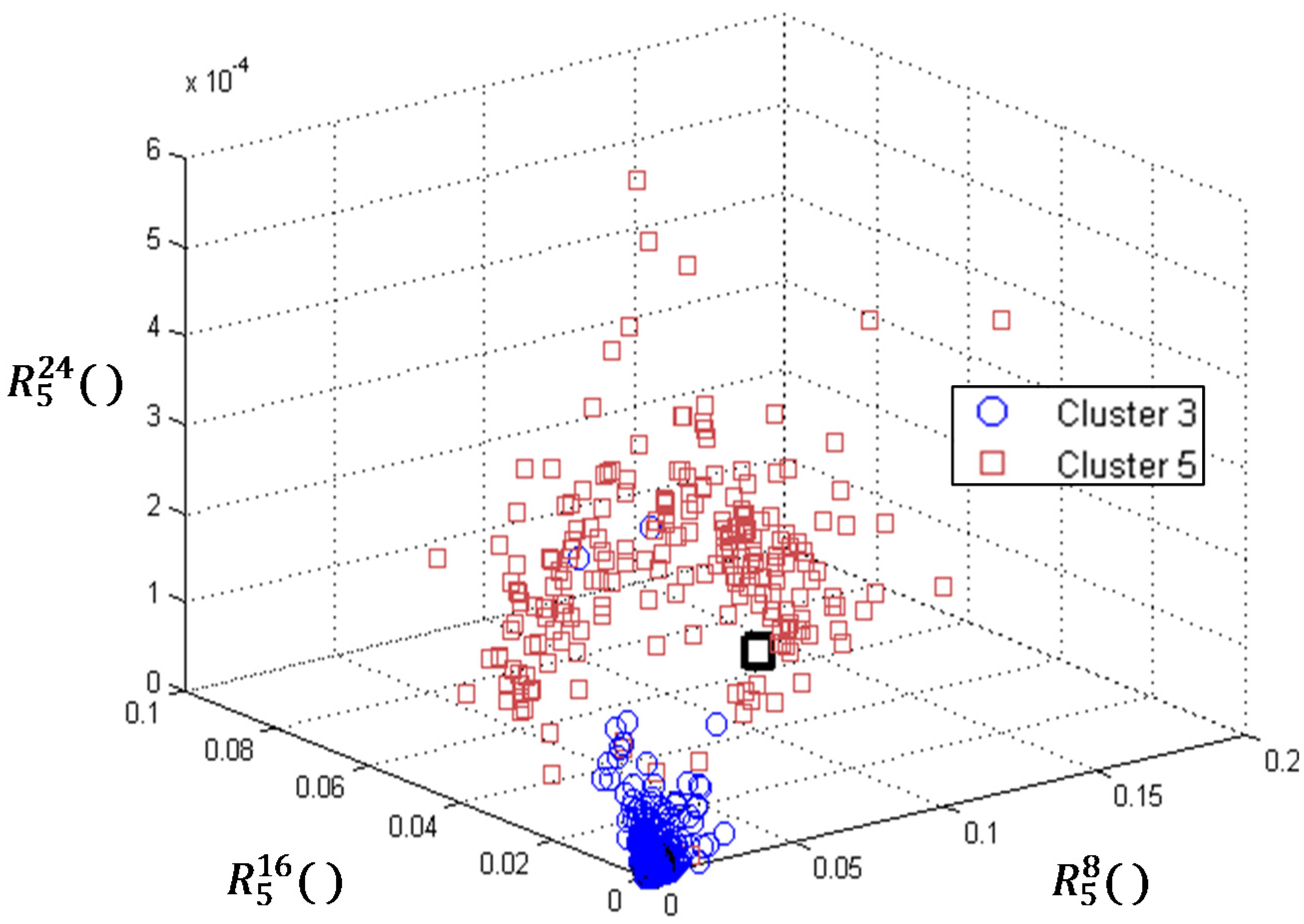
Figure 6. Visualization of feature vectors designated as cluster 3 and 5.

Figure 6. Visualization of feature vectors designated as cluster 3 and 5.

Figure 6 show feature vectors representing process-orientated AE bursts (cluster 3) and feature vectors indicating damage (cluster 5) during the holding stage of the injection molding process. Axes of 3D plot are normalization values of wavelet packets energy at 5th resolution. A black circle indicates the position of the feature vector of the AE burst from Figure 4a and a black square the position of the feature vector of the AE burst from Figure 4b. Cluster 3 feature vectors are concentrated around the origin of the coordinate system while Cluster 5 feature vectors are spread away from the origin.

3.3. SFS Feature Selection

The dimensions of the feature vector cannot be arbitrary large. One reason is the computational complexity, and the second reason is that the dimension ultimately causes a decrease of performance [14,24]. Our goal is to reduce the dimensions of the data by finding a small set of important features that can give good classification performance. With feature selection we find a subset F_j(W) = {z_w|w=1, ..., W} that outperforms all other subsets with dimension W as:

J(F_i(W)) ≥ J(F_j(W)) for all jϵ{1, …, q(W)}

(19)

where q(W) is the number of evaluations of performance measure J(F_j(W)).

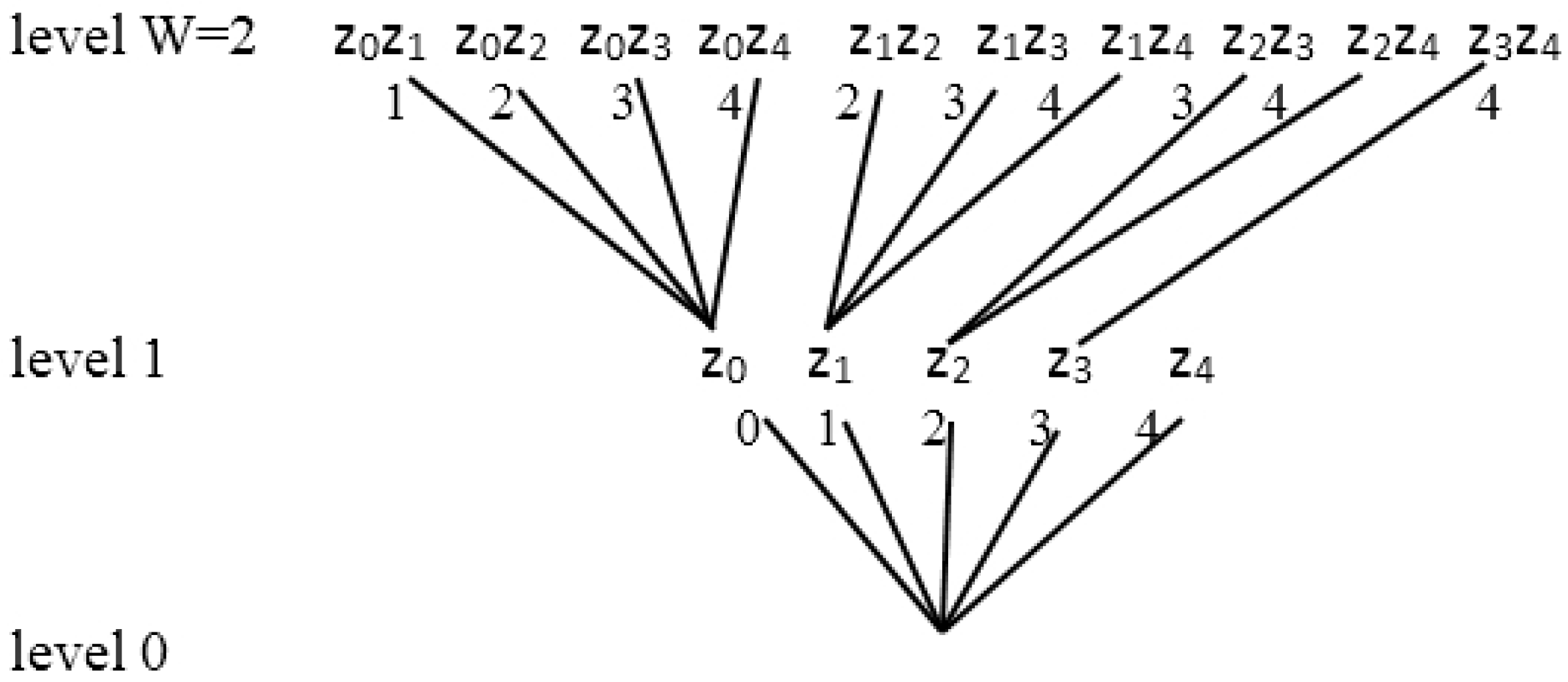
We used sequential forward selection (SFS). The method starts at the bottom (the root of the tree) with an empty set and proceeds its way to the top without backtracking. At each level of the tree, SFS adds one feature to the current feature set by selecting from the remaining available measurements the element that yields a maximal increase of the performance. A structure of feature selection is shown in Figure 7, where z_n is the designation of a feature.

Figure 7. A bottom-up tree structure for feature selection [24].

Figure 7. A bottom-up tree structure for feature selection [24].

We used a k-Nearest Neighbor (k-NN) classification algorithm as a criterion. With k-NN the input consists of the k closest training examples in the feature space. In our research k = 3. The output of the algorithm is a class membership. An object is classified by a majority vote of its neighbors, with the object being assigned to the class most common among its k nearest neighbors.

The major focus of our research was detection of damage in an injection molding tool during the injection molding process. This was the reason for using SFS with k-NN on feature vectors of AE burst signals acquired during the holding phase of the injection molding cycle on intact and damaged molds. We selected feature subset Z_s with a size of 10. Feature subset was used for neural network pattern recognition of AE signals during the full time of the injection molding cycle. The selected features based on SFS with k-NN are: Z_s = ($R_5^8$, $R_5^{16}$, $R_5^{24}$, $R_5^{21}$, $R_5^{18}$, $R_5^{20}$, d, $R_5^6$, $R_5^{32}$, A_p).

3.4. Classification of All Input Vectors Based on AE Signals

For the purposes of presenting all feature vectors Z, we introduced principal component analysis (PCA) as an unsupervised feature reduction method. PCA offers us transformation of high-dimensional feature vector Z to a much lower dimensional vector i.e., P. PCA is mathematically defined [25] as an orthogonal linear transformation that transforms the data into a new coordinate system such that the greatest variance by some projection of the data comes to lie on the first coordinate (called the first principal component), the second greatest variance on the second coordinate, and so on. 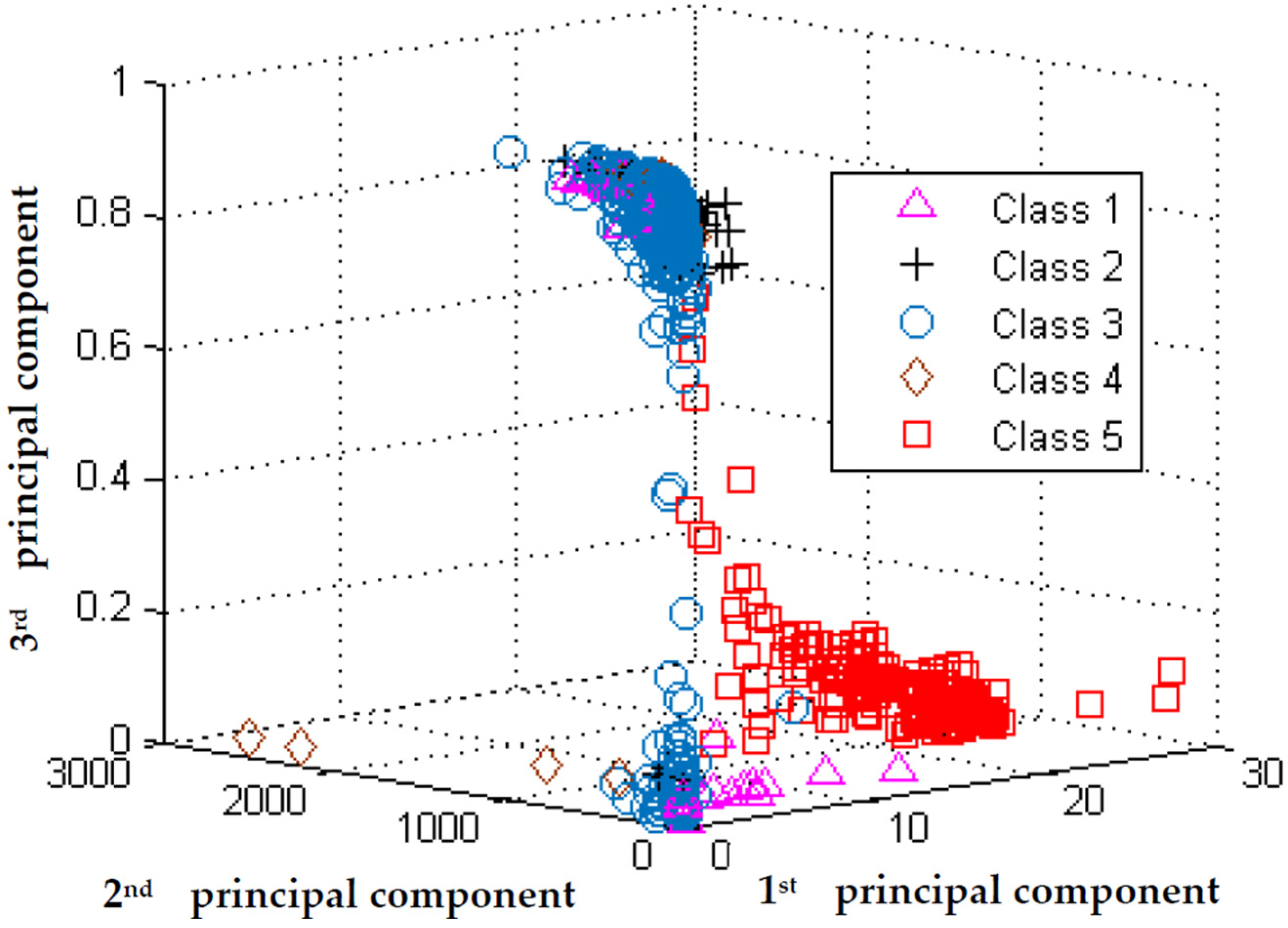Figure 8 shows the distribution of feature vectors Z in a 3D coordinate system of the first three principal components. Feature vectors Z are divided into five classes; Class 1—the closing of the mold, Class 2—the injection of the melt with maximum pressure, Class 3—holding (packing) stage, Class 4—opening of the tool, Class 5—AE signals characterizing damage of the tool.

Figure 8. PCA visualization of all feature vectors Z during injection molding cycles.

Figure 8. PCA visualization of all feature vectors Z during injection molding cycles.

Based on the measured AE bursts, we set 10-dimensional feature subset vector Z_s with instances that are real-valued descriptors (variables). Vector Z_s offers us defining points in appropriate multidimensional space to characterize the process. We used a classification to identify the categories or sub-populations based on a training dataset, containing instances whose category membership is known. The training data consist of a set of 704 input vectors Zs that have been designated based on the time moment of their acquisition during the injection molding cycle and unsupervised FCM for vectors of the damaged tool. For neural network pattern recognition we used a feed-forward network with the F Tan-Sigmoid transfer function in both the hidden and the output layer. We used 10 neurons in the hidden layer and five output neurons, because there are five target categories associated with each input vector. The network is trained with scaled conjugate gradient back-propagation.

Table 1. Classification of all input vectors in all confusion matrix.

All Confusion Matrix
Output Class	1	8	0	1	0	3	33.3%
		1.1%		0.1%		0.4%
	2	0	27	0	4	0	12.9%
			3.8%		0.6%
	3	32	0	378	8	4	10.4%
		4.5%		53.7%	1.1%	0.6%
	4	0	3	1	26	0	13.3%
			0.4%	0.1%	3.7%
	5	2	0	1	0	206	1.4%
		0.3%		0.1%		29.3%
	E	81.0%	10.0%	0.8%	31.6%	3.3%	8.4%
	o.c./t.c.	1	2	3	4	5	E
		Target Class

E—Means error.

Table 1. Classification of all input vectors in all confusion matrix.

All Confusion Matrix
Output Class	1	8	0	1	0	3	33.3%
		1.1%		0.1%		0.4%
	2	0	27	0	4	0	12.9%
			3.8%		0.6%
	3	32	0	378	8	4	10.4%
		4.5%		53.7%	1.1%	0.6%
	4	0	3	1	26	0	13.3%
			0.4%	0.1%	3.7%
	5	2	0	1	0	206	1.4%
		0.3%		0.1%		29.3%
	E	81.0%	10.0%	0.8%	31.6%	3.3%	8.4%
	o.c./t.c.	1	2	3	4	5	E
		Target Class

E—Means error.

For training of our network, data were randomly distributed into three subsets. A training subset (70% of the data) is used for computing the gradient and updating the network weights W and biases B. In the validation subset (15% of the data) the error is monitored during the training process. The network weights and biases are saved at the minimum of the validation subset error. The testing subset (15% of the data) has no effect on training but provides an independent measure of network performance during and after training. The results of classification of all input data are shown in Table 1. The table has five output classes (o.c.) and five target classes (t.c.) with a number of vectors classified into appropriate classes.

The presented data show that we have on average 91.6% correctly classified subset feature vectors Z_s. The lowest error E = 0.8% is for Class 3 vectors, representing process-orientated AE signals during the holding (packing) stage. Detection of damage (Class 5) in the injection molding tool is 96.7% correct. Misclassified vectors representing damage are almost evenly distributed between Class 1 and 3. The highest error, 81%, is for detection of tool closing, i.e., Class 1 vectors Z_s. Also, the class 4 vectors representing opening of the tool show relatively high error E = 31.6%.

4. Conclusions

In this work we presented an AE monitoring system with a resonant sensor that is able to detect the damaged area in an injection molding tool. We made a close comparison of AE signals captured from a new mold and a damaged mold under the same injection molding process conditions.

The most useful information about the injection molding tool integrity based on AE bursts is gained during the filling and holding stage of the injection molding process, when the mold pressure is high enough.

We introduced time domain, frequency domain, and wavelet packet transform descriptors to classify feature vectors of AE bursts during the injection molding cycle. A 10-dimensional subset feature vector with real-valued explanatory variables is proposed for classification of AE burst signals.

Based on SFS, the feature subset consists mainly of normalization values of the energy of wavelet packets, which turned out to be the most informative for prediction of damaged areas in the injection molding tool.

Neural network pattern recognition results show very good prediction probability of tool damage and very good prediction of process-orientated signals during the filling and holding phases of the injection molding cycle.