Distributed Global Function Model Finding for Wireless Sensor Network Data

Abstract

Function model finding has become an important tool for analysis of data collected from wireless sensor networks (WSNs). With the development of WSNs, a large number of sensors have been widely deployed so that the collected data show the characteristics of distribution and mass. For distributed and massive sensor data, traditional centralized function model finding algorithms would lead to a significant decrease in performance. To solve this problem, this paper proposes a distributed global function model finding algorithm for wireless sensor network data (DGFMF-WSND). In DGFMF-WSND, on the basis of gene expression programming (GEP), an adaptive population generation strategy based on sub-population associated evolution is applied to improve the convergence speed of GEP. Secondly, to solve the generation of global function model in distributed wireless sensor networks data, this paper provides a global model generation algorithm based on unconstrained nonlinear least squares. Four representative datasets are used to evaluate the performance of the proposed algorithm. The comparative results show that the improved GEP with adaptive population generation strategy outperforms all other algorithms on the average convergence speed, time-consumption, value of R-square, and prediction accuracy. Meanwhile, experimental results also show that DGFMF-WSND has a clear advantage in terms of time-consumption and error of fitting. Moreover, with increasing of dataset size, DGFMF-WSND also demonstrates good speed-up ratio and scale-up ratio.

1. Introduction

Progress in wireless communication and microelectronic devices has led to the development of low-power sensors and the deployment of large-scale sensor networks [1]. Wireless sensor networks (WSNs) have been developed and applied to many fields, such as smart grid [2], agriculture [3,4], environment monitoring [5,6], and the military [7]. In these applications, because of the large number and wide distribution of sensors, the data from sensors is characterized by high dimension, large amount, and wide distribution [8,9]. How to find useful knowledge from high dimensional, massive and distributed data has become a key issue of data mining in wireless sensor networks [8,9].

Recently, all kinds of approaches, including clustering [10,11], association rules [12] and classification [13,14], have been successfully applied in wireless sensor networks. Function model finding is also an important branch of data mining. The function finding technique for all kinds of application data from WSNs can reveal the essence and phenomenon in the application. However, in the existing references, function finding is rarely mentioned in WSNs.

The existing function model discovery algorithms mainly include the regression, the evolution algorithms, and so on. Generally, traditional regression methods assumed that the function type was known, and then the least squares method or its improved methods for parameter estimation were used to determine the functional model [15]. These traditional regression methods needed to depend on a priori knowledge and a lot of subjective factors. Moreover, these methods have high time complexity and low computation efficiency for complex and high-dimensional datasets from WSNs. To solve these problems, Li et al. and Koza et al. used genetic programming (GP) for mathematical modeling and obtained good experimental results [16,17]. Yeun et al. proposed a method which dealt with smooth fitting problem by GP [18]. In order to fit data points to curves in CAD (Computer Aided Design)/CAM (Computer Aided Manufacturing), Gálvez et al. present a new hybrid evolutionary approach (GA-PSO) for B-spline curve reconstruction [19]. Meanwhile, GP, genetic algorithm (GA) or hybrid evolutionary algorithms also avoid the defect of traditional statistical methods’ selected function models in advance. However, the efficiency of function model mined by GP, GA or hybrid evolutionary algorithms was low. Thus, a new algorithm called gene expression programming (GEP) was proposed [20]. Compared with GP, the efficiency of complex functions mined based on GEP was improved 4–6 times.

Therefore, in order to reveal the inherent nature of the sensor data, this paper proposes a function finding algorithm using gene expression programming (FF-GEP). In FF-GEP, an adaptive population generation strategy is put forward. The strategy avoids the local optimum of GEP population. However, thousands of distributed sensor nodes, and the unstable wireless communication environment make traditional centralized function mining algorithms difficult to meet the needs of function mining in wireless sensor networks. Traditional centralized FF-GEP is unable to meet the requirement of function finding in wireless sensor networks. In order to better find functions for complex, massive and high-dimensional sensor data, on the basis of FF-GEP, this paper presents distributed global function model finding for wireless sensor networks data (DGFMF-WSND).

The main contributions of this paper are summarized as follows: (1) we present the function finding algorithm using gene expression programming for wireless sensor networks data (FF-GEP) in order to prevent GEP from the local optimum; (2) we solve the generation of the global function model in distributed function finding and provide a global model generation algorithm based on unconstrained and nonlinear least squares (GMG-UNLS); (3) on the basis of FF-GEP and GMG-UNLS, we put forward distributed global function model finding for wireless sensor networks data (DGFMF-WSND); and (4) we describe simulated experiments that have been done and provides performance analysis results.

The content of the paper is organized as follows. Section 2 discusses prior work related to data mining in WSNs and function mining. Section 3 introduces the function finding algorithm using gene expression programming for wireless sensor networks data. Section 4 emphasizes the distributed global function model finding for wireless sensor networks data. Section 5 represents experiments and performance analysis. Finally, conclusions are given in Section 6.

2. Related Work

2.1. Data Mining in Wireless Sensor Networks (WSNs)

Recently, mining knowledge from sensor data has attracted a great deal of attention from data mining experts [21]. Lee et al. proposed a fuzzy-logic-based clustering approach to prolong the lifetime of WSNs using energy predication [10]. Liu et al. present a distributed energy-efficient clustering algorithm with improved coverage by analyzing communication energy consumption of the clusters and the impact of node failures on coverage with different densities in wireless sensor networks [11]. In WSNs, the stream nature of the data, the limited resources, and the distributed nature of sensor networks bring new challenges for the mining techniques. Boukerche et al. proposed a new formulation for the association rules [12]. In these references, data mining techniques are only seen as a means to solve the problems existing in WSNs. Generally, for data mining in wireless sensor networks, WSNs would be regarded as platform of data collection and transmission [22]. Finally, we analyzed these data from WSNs. Due to the wide range of application of WSNs, the analysis and mining of all kinds of data based on wireless sensor network are also emphasized. Sawaitul et al. proposed classification and prediction of future weather using Back Propagation (BP) Algorithm for data collected by weather sensors [23]. Erdogan et al. present a data mining approach for fall detection using k-nearest neighbor algorithm on wireless sensor network data in order to enhance life safety of the elderly and boost their confidence [24]. Tripathy et al. present knowledge discovery and leaf spot dynamics of groundnut crop by wireless sensor network and data mining techniques. The useful information, knowledge or relations from all kinds of data mining techniques would be helpful to analyze and understand leaf spot disease infection [25]. In order to protect sensor nodes from malicious attacks, Huang et al. proposed a new intrusion detection method. The method constructed Markov decision processes based on an attack pattern mining in order to predict future attack patterns and implement appropriate measures [26]. In order to explore, analyze, and extract useful information and knowledge from the larger number of personal data which came from smartphone and wearable devices, Muhammad et al. proposed the personal ecosystem where all computational resources, communication facilities, storage and knowledge management systems are available in user proximity [27]. As suggested above, it can be seen that finding knowledge or model from wireless sensor network data is very meaningful and valuable.

2.2. Function Mining

At present, research on GEP focused on the basic theory of algorithm, symbolic regression, function finding, prediction, security assessment, other application areas, and so forth. In algorithm theory, in order to solve the problem that fitness distance correlation could hardly predict the evolution difficulty of gene expression programming, Zheng et al. proposed gene expression programming evolution difficulty prediction based on posture model [28]. Ryan et al. simplified operators of GEP and proposed a robust gene expression programming algorithm [29]. Zhu et al. present naive gene expression programming (NGEP) based on genetic neutrality that combined with neutral theory of molecular evolution [30]. In symbolic regression and function mining, Peng et al. proposed an improved GEP algorithm named S_GEP, which is especially suitable for dealing with symbolic regression problems [31]. To better improve efficiency and accuracy of classification, Karakasis et al. proposed a hybrid evolutionary technique by combining GEP with artificial immune system [32]. In order to better model the compressive strength of different types of geopolymers, GEP had been employed. The model showed that GEP had a strong potential for predicting the compressive strength of different types of geopolymers [33]. In view of insufficiency of the existing forecasting model on highway construction cost forecasting, highway construction cost forecasting model was proposed based on the GEP according to the characteristic of highway construction cost forecasting [34]. Güllü proposed a function finding algorithm by gene expression programming for strength and elastic properties of clay treated with bottom ash in order to understand the treatment of a marginal soil well [35]. Zhao et al. treated image registration as a formula discovery problem, and proposed two-stage gene expression programming and the improved cooperative particle swarm optimizer used to identify the registration formula for the reference image and the floating image [36]. In prediction, Lee et al. posed gene expression programming on Taiwan stock investment [37]. Mousavi et al. proposed the prediction of electricity demand based on GEP [38]. Chen et al. applied parallel hyper-cubic gene expression programming to estimate the slump flow of high-performance concrete [39]. Huo et al. applied gene expression programming to short-term load forecasting on power systems, and proposed the model error cycling compensation [40]. Forecasting results indicated that the model was of high prediction efficiency. Seyyed et al. used gene expression programming to design a new model for the prediction of compressive strength of high performance concrete (HPC) mixes [41]. Experiments showed that prediction performance of the optimal GEP model is better than the regression models. In security assessment and other application areas, Khattab et al. introduced gene expression programming into power system static security assessment [42]. To better design sensor equivalent circuit, Janeiro et al. used GEP to determine a suitable equivalent circuit and choose a circuit component [43]. For combinatorial optimization problems, Sabar et al. present a dynamic multiarmed bandit-gene expression programming hyper-heuristic [44]. Zhang et al. provided revised gene expression programming to construct the model for music emotion recognition [45]. However, these algorithms do not involve distributed function mining.

3. Function Finding Algorithm by Using Gene Expression Programming for Wireless Sensor Networks Data

3.1. Function Finding in Wireless Sensor Networks

Generally, for data mining in wireless sensor networks, firstly, data are collected and preprocessed by various sensors and transmitted directly to the servers by means of wireless communication. Then, these data can be quickly analyzed by strong data processing and analysis ability of servers. Finally, the knowledge is attained. The whole framework is shown in Figure 1.

Figure 1. Data mining framework in wireless sensor networks.

Figure 1. Data mining framework in wireless sensor networks.

From Figure 1, it is known that data mining for wireless sensor networks consists of five main components: acquisition layer, preprocessing layer, transmission layer, analysis layer and virtualization layer. The acquisition layer is responsible for collecting all kinds of data (e.g., weather, spectral, temperature, humidity, gas, etc.) through various sensors (e.g., weather sensor, hyperspectral sensor, temperature sensor, humidity sensor, gas sensor, etc.). The preprocessing layer focuses on data aggregation, normalization and cleaning to provide favorable data form for data mining in wireless sensor networks. The transmission layer mainly addresses security transmission of data between sensors and terminals. The analysis layer provides all types of data mining services for data from various sensors. Finally, the results of data mining are shown by the virtualization layer.

Function discovery is an important part of data mining framework in wireless sensor networks. It is vital to find the function model among sensor data for the concrete application and analysis on WSNs. This paper proposes function finding algorithm using gene expression programming (FF-GEP) for sensor data. The details are shown as follows.

3.2. Coding of Gene Expression Programming (GEP)

The gene is the basic unit of GEP [20]. In order to better describe GEP algorithm, the related definitions are given as follows.

Definition 1. Let string $G$ be defined as a triplet $G=<GHead,GTail,L>$, $F$ be basic elementary function set and $T$ be terminal set. Where $GHead$, $GTail$ and $L$ represent head, tail, length of the $G$ respectively. The elements of $GHead$ randomly generates from $F$ and $T$, the elements of $GTail$ randomly generates from $T$. Then string $G$ is called gene.

Property 1. Let the length of $GHead$ be $h$, the length of $GTail$ be $t$, maximum number of arguments of operator in the $GHead$ be $n$. Then, $h$ and $t$ follow the equation:

$$t=h\times (n-1)+1$$

(1)

Definition 2. The string which is composed of one or more $G$ is called the chromosome, and denoted as $C$.

GEP adopts linear code of fixed length to represent an individual which is called a chromosome $C$. However, the linear code can accurately show expression trees (ETs) of different shapes and sizes. During decoding, firstly, ETs is traversed from the upper to the bottom, the left to the right, and finally, function model is obtained.

Example 1. Let function set be $F=\{+,-,\times ,Q\}$, terminal set be $T=\{a,b\}$, length of gene head be $h=5$, where “$Q$” represents the square root function. From function set $F$, we know that maximum number of arguments of all operators is 2. According to Equation (1), length of gene tail is 6. The randomly generated chromosome is shown in Figure 2.

Figure 2. A random chromosome in gene expression programming (GEP).

Figure 2. A random chromosome in gene expression programming (GEP).

The chromosome shown in Figure 2 consists of two genes. The corresponding expression trees (ETs) is shown in Figure 3.

Figure 3. The corresponding expression trees.

Figure 3. The corresponding expression trees.

The decoding of Sub-ET₁ and Sub-ET₂ is respectively performed. The result of decoding is linked by addition function and simplified by mathematica software. The final function model is $f\left(a,b\right)=3a+ab+\frac{1}{b}-\sqrt{b}$.

3.3. Adaptive Population Generation Strategy Based on Collaborative Evolution of Sub-Population

In GEP, in order to better evolve, gene diversity in the initial population is required so that the GEP algorithm can evolve from different directions. At present, the strategy of initial population generation is simple and occupies fewer system resources. However, the diversity of the population generated by the strategy is limited. With the increasing of fitness value of an individual, it is easy to stop the population evolving and fall into local optimum. In theory, the greater the population space, the more diverse the individual, the greater the probability of searching the global optimal solution. However, increase of population space will increase the computational complexity and reduce the convergence speed. Thus, in order to prevent the population from falling into local optimum, this paper presents an adaptive population generation strategy based on collaborative evolution of sub-population (APGS-CESP). In APGS-CESP, the probability of searching the global optimal solution is increased by raising the diversity of the individuals in the population. The flow of APGS-CESP is shown as follows.

Algorithm 1. APGS-CESP ($Pop$)

Input: Pop, $P_s$, $P_m$, $P_t$, $P_r$, popSize;

Output: new Population;

Begin {

1. for (int i = 1; i <= MaxGen; i++){

2. $F_{\max }[i]$ = MaxFitness (Pop [i]);

3. $Sum{F}_{\max }$ = 0; $Sum{F}_{\max }+=F_{\max }[i]$;

4. if ($i\mathrm{mod}10==0$){

5. if ($sum{F}_{max}\mathrm{mod}10==0$) {

6. $subPop\leftarrow RandomInitPop(subPopSize)$;

7. $Pop\leftarrow Insert(subPop,Pop)$;

8. $EvalueFitness(Pop)$;

9. $Pop\leftarrow Select(P_s,Pop,popSize)$;

10. $Pop\leftarrow Mutate(P_m,Pop)$;

11. $Pop\leftarrow ISTransposition(P_t,Pop)$;

12. $Pop\leftarrow RISTransposition(P_t,Pop)$;

13. $Pop\leftarrow GeneTransposition(P_t,Pop)$;

14. $Pop\leftarrow OnePointRecombination(P_r,Pop)$;

15. $Pop\leftarrow TwoPointRecombination(P_r,Pop)$;

16. $Pop\leftarrow GeneRecombination(P_r,Pop)$;}}}

17. $newPopulation=Pop$;

18. Return newPopulation;}

Generally, Algorithm 1 enriches diversity of the individuals in the population, and expands the scope of the global optimal solution. However, size of the population has not increased and time complexity of the algorithm changes from $O(popSize)$ to $O(popSize+subPopSize)$.

3.4. Description of Function Finding Algorithm Using Gene Expression Programming (FF-GEP)

GEP has strong global searching ability. Therefore, it has definite potential in getting sufficiently good solutions to function model finding problems for wireless sensor network data. The core of FF-GEP focuses on putting adaptive population generation strategy into population evolution. The steps of FF-GEP are shown as follows:

Algorithm 2. FF-GEP

Input: popSize, maxGen, maxFitness, $P_s$, $P_m$, $P_t$, $P_r$;

Output: Best Function Expression;

Begin {

1. double $fitness=0.0$; int $i=0$;

2. $Pop\leftarrow InitPop(popSize)$;

3. $EvalueFitness(Pop)$;

4. while (($fitness\le maxFitness$) or ($i\le maxGen$)) {

5. $Pop\leftarrow Select(P_s,Pop,popSize)$;

6. $Pop\leftarrow Mutate(P_m,Pop)$;

7. $Pop\leftarrow ISTransposition(P_t,Pop)$;

8. $Pop\leftarrow RISTransposition(P_t,Pop)$;

9. $Pop\leftarrow GeneTransposition(P_t,Pop)$;

10. $Pop\leftarrow OnePoint\mathrm{Re}combination(P_r,Pop)$;

11. $Pop\leftarrow TwoPoint\mathrm{Re}combination(P_r,Pop)$;

12. $Pop\leftarrow Gene\mathrm{Re}combination(P_r,Pop)$;

13. $Pop\leftarrow APGS-SPAE(Pop)$;

14. $EvalueFitness(Pop)$;}

15. return BestFunctionExpression;}

4. Distributed Global Function Model Finding for Wireless Sensor Networks Data

4.1. Algorithm Idea

In WSNs, because the number of sensors is very large and sensors are physically deployed in a very distributed fashion, traditional centralized function model finding algorithms will undoubtedly increase transmission bandwidth, network delay and probability of data packet loss, and also reduce the efficiency of function model finding. Meanwhile, centralized analysis for massive data in WSNs will also add pressure to the data storage so that traditional centralized function model finding algorithms are difficult to apply in wireless sensors networks.

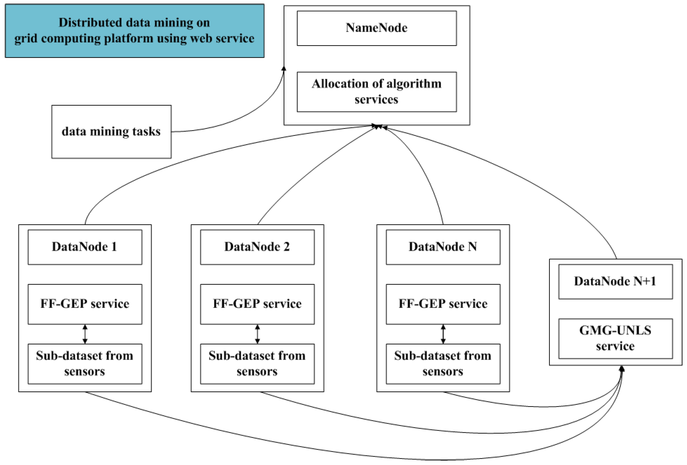
Grid is a high performance and distributed computing platform with good self-adaptability and scalability, and provides favorable computing and analysis capability for massive or distributed data sets. Grid could provide strong analysis and computing power with distributed data mining and knowledge discovery. In view of advantages of grid computing, on the basis of FF-GEP, this paper presents distributed global function model finding for wireless sensor networks data (DGFMF-WSND) which combines with global model generation and grid services.

Suppose that data on each grid node are homogeneous and the attributes that are contained in each of datasets on the computing nodes are same in this paper. The algorithm idea is divided into some sub-processes. Firstly, algorithms proposed in this paper are wrapped as grid services and deployed on each grid node. Meanwhile, a local function model is obtained by performing FF-GEP algorithm service on each grid node in parallel. Lastly, the local function model of each node is transmitted to the specified node to generate a global model and returned to the user.

4.2. Global Model Generation Algorithm Based on Unconstrained Nonlinear Least Squares

The traditional distributed data mining algorithm mainly includes two steps: (1) analyzing local data and generating a local function model; (2) global function model is obtained by integrating different local function models. How to get the global function model from the local function model has not been investigated in earlier work. This paper presents a global model generation algorithm based on unconstrained nonlinear least squares (GMG-UNLS).

Definition 3. In WSNs, we propose the number of the sensor node and sink node are k and n, respectively. For each sink node, it contains a sensor data set $S=[x_1,\mathrm{...},x_m\text{\hspace{0.17em}}{y}_{m+1}]$, where $S\in R^{m+1}$ and $y_{m+1}$ represents target value for each sensor data set. Then, the set of each sink node can be obtained yielding to GEP by employing the approach of function model mining, such that $y_i(x_{m+1})=f_i(x_1,x_2,\mathrm{...},x_m),i\in [1,n]$. Hence, $y_i(x_{m+1})=f_i(x_1,x_2,\mathrm{...},x_m)$ is the local function model with m-dimension of the i-th sink node.

Definition 4. Suppose that there exist n sink nodes and $f_i(X),i\in [1,n]$, where $X=(x_1,x_2,\mathrm{...},x_m)$. There exists a set of constants $a_i\ne 0,i\in [1,n]$ such that $f(x_1,x_2,\mathrm{...},x_m)={\displaystyle \sum _{i=1}^n{a}_i{f}_i(X)}$. Thus, $f(x_1,x_2,\mathrm{...},x_m)$ is called global function model.

Lemma 1. 

Given that there exist n local function model $f_1(x_1,x_2,\mathrm{...},x_m),,\mathrm{...},f_n(x_1,x_2,\mathrm{...},x_m)$ with m-dimension in WSNs, and $(m+1)\times p$ sample datasets on each sink node. There exists a set of constants $a_i\ne 0,i\in [1,n]$ such that value of ${\displaystyle \sum _{i=1}^k{(y_i-{\displaystyle \sum _{j=1}^n{a}_j{f}_j(X_i)})}^2}$ is minimum, where $k=np$.

Proof: 

Set $Q(a_1,a_2,\mathrm{...},a_n)={\displaystyle \sum _{i=1}^k{(y_i-{\displaystyle \sum _{j=1}^n{a}_j{f}_j(X_i)})}^2}$. Then

$$\begin{array}{ll}Q(a_1,a_2,\mathrm{...},a_n)\hfill & ={\displaystyle \sum _{i=1}^k{(a_1{f}_1(X_i)+a_2{f}_2(X_i)+\mathrm{...}+a_n{f}_n(X_i)-y_i)}^2}\hfill \\ & ={(a_1{f}_1(X_1)+\mathrm{..}+a_n{f}_n(X_1)-y_1)}^2+\mathrm{...}+{(a_1{f}_1(X_k)+\mathrm{..}+a_n{f}_n(X_k)-y_k)}^2\hfill \end{array}$$

(2)

where $f_j(X_i),i\in [1,k]\text{\hspace{0.17em}},j\in [1,n]$ and $y_1,\mathrm{...},y_k$ are constants. Denote

$$f_1(X_1)=C_{11},f_2(X_1)=C_{21},\mathrm{...},f_n(X_1)=C_{n1},\mathrm{...},f_1(X_k)=C_{1k},f_2(X_k)=C_{2k},\mathrm{...},f_n(X_k)=C_{nk}$$

(3)

Substituting Equation (3) into Equation (2), we have that

$$Q(a_1,a_2,\mathrm{...},a_n)={(a_1{C}_{11}+\mathrm{..}+a_n{C}_{n1}-y_1)}^2+\mathrm{...}+{(a_1{C}_{1k}+\mathrm{..}+a_n{C}_{nk}-y_k)}^2$$

(4)

Because $Q(a_1,a_2,\mathrm{...},a_n)$ is a two time polynomial of $(a_1,a_2,\mathrm{...},a_n)$, and composed of basic elementary functions, and differentiable.

Hence, the partial derivative of $Q(a_1,a_2,\mathrm{...},a_n)$ with respect to $a_1,a_2,\mathrm{...},a_n$ exists, respectively. The Equations (5)–(7) hold.

$$\frac{\partial Q}{\partial a_1}=2(a_1{\displaystyle \sum _{i=1}^k{C}_{1i}^2}+a_2{\displaystyle \sum _{i=1}^k{C}_{1i}{C}_{2i}+\mathrm{...}+a_n{\displaystyle \sum _{i=1}^k{C}_{1i}{C}_{ni}}}-{\displaystyle \sum _{j=1}^k{y}_j{C}_{1j}})$$

(5)

$$\frac{\partial Q}{\partial a_2}=2(a_1{\displaystyle \sum _{i=1}^k{C}_{2i}{C}_{1i}}+a_2{\displaystyle \sum _{i=1}^k{C}_{2i}^2+\mathrm{...}+a_n{\displaystyle \sum _{i=1}^k{C}_{2i}{C}_{ni}}}-{\displaystyle \sum _{j=1}^k{y}_j{C}_{2j}})$$

(6)

$$\frac{\partial Q}{\partial a_n}=2(a_1{\displaystyle \sum _{i=1}^k{C}_{ni}{C}_{1i}}+a_2{\displaystyle \sum _{i=1}^k{C}_{ni}{C}_{2i}+\mathrm{...}+a_n{\displaystyle \sum _{i=1}^k{C}_{ni}^2}}-{\displaystyle \sum _{j=1}^k{y}_j{C}_{nj}})$$

(7)

Solving $(a_1,a_2,\mathrm{...},a_n)$ such that value of $Q(a_1,a_2,\mathrm{...},a_n)$ is minimum. Set $\frac{\partial Q}{\partial a_i}=0,i\in [1,n]$. Thus, Equation (8) can be obtained.

$$\left[\begin{array}{cccc}{\displaystyle \sum _{i=1}^k{C}_{1i}^2}& {\displaystyle \sum _{i=1}^k{C}_{1i}{C}_{2i}}& \mathrm{...}& {\displaystyle \sum _{i=1}^k{C}_{1i}{C}_{ni}}\\ {\displaystyle \sum _{i=1}^k{C}_{2i}{C}_{1i}}& {\displaystyle \sum _{i=1}^k{C}_{2i}^2}& \mathrm{...}& {\displaystyle \sum _{i=1}^k{C}_{2i}{C}_{ni}}\\ \mathrm{...}& \mathrm{...}& \mathrm{...}& \mathrm{...}\\ {\displaystyle \sum _{i=1}^k{C}_{ni}{C}_{1i}}& {\displaystyle \sum _{i=1}^k{C}_{ni}{C}_{2i}}& \mathrm{...}& {\displaystyle \sum _{i=1}^k{C}_{ni}^2}\end{array}\right]\left[\begin{array}{c}{a}_1\\ a_2\\ \mathrm{...}\\ a_n\end{array}\right]=\left[\begin{array}{c}{\displaystyle \sum _{j=1}^k{y}_j{C}_{1j}}\\ {\displaystyle \sum _{j=1}^k{y}_j{C}_{2j}}\\ \mathrm{...}\\ {\displaystyle \sum _{j=1}^k{y}_j{C}_{nj}}\end{array}\right]$$

(8)

Denote

$$\left[\begin{array}{cccc}{\displaystyle \sum _{i=1}^k{C}_{1i}^2}& {\displaystyle \sum _{i=1}^k{C}_{1i}{C}_{2i}}& \mathrm{...}& {\displaystyle \sum _{i=1}^k{C}_{1i}{C}_{ni}}\\ {\displaystyle \sum _{i=1}^k{C}_{2i}{C}_{1i}}& {\displaystyle \sum _{i=1}^k{C}_{2i}^2}& \mathrm{...}& {\displaystyle \sum _{i=1}^k{C}_{2i}{C}_{ni}}\\ \mathrm{...}& \mathrm{...}& \mathrm{...}& \mathrm{...}\\ {\displaystyle \sum _{i=1}^k{C}_{ni}{C}_{1i}}& {\displaystyle \sum _{i=1}^k{C}_{ni}{C}_{2i}}& \mathrm{...}& {\displaystyle \sum _{i=1}^k{C}_{ni}^2}\end{array}\right]=B,\left[\begin{array}{c}{a}_1\\ a_2\\ \mathrm{...}\\ a_n\end{array}\right]=X,\text{\hspace{0.17em}and\hspace{0.17em}}\left[\begin{array}{c}{\displaystyle \sum _{j=1}^k{y}_j{C}_{1j}}\\ {\displaystyle \sum _{j=1}^k{y}_j{C}_{2j}}\\ \mathrm{...}\\ {\displaystyle \sum _{j=1}^k{y}_j{C}_{nj}}\end{array}\right]=Y$$

Then Equation (8) can be rewritten as $BX=Y$. Because of the randomness of data acquisition and function model finding using GEP in wireless sensor networks, there are no two identical or proportional row vectors in the matrix B so that the determinant of matrix B is not equal to 0. According to definition of rank of a matrix, we have that $R\left(B\right)=R\left(B|Y\right)=n$. Therefore, non homogeneous linear equations $BX=Y$ exist unique solution $(a_1,a_2,\mathrm{...},a_n)$. According to the theorem and deduction of the corresponding calculation of determinant [46], we have that $(a_1,a_2,\mathrm{...},a_n)=(\frac{d_1}{d},\frac{d_2}{d},\mathrm{...},\frac{d_n}{d})$, where

$$d_j=\left|\begin{array}{ccccccc}{\displaystyle \sum _{i=1}^k{C}_{1i}^2}& \cdots & {\displaystyle \sum _{i=1}^k{C}_{1i}{C}_{j-1,i}}& {\displaystyle \sum _{j=1}^k{y}_j{C}_{1j}}& {\displaystyle \sum _{i=1}^k{C}_{1i}{C}_{j+1,i}}& \cdots & {\displaystyle \sum _{i=1}^k{C}_{1i}{C}_{ni}}\\ {\displaystyle \sum _{i=1}^k{C}_{2i}{C}_{1i}}& \cdots & {\displaystyle \sum _{i=1}^k{C}_{2i}{C}_{j-1,i}}& {\displaystyle \sum _{j=1}^k{y}_j{C}_{2j}}& {\displaystyle \sum _{i=1}^k{C}_{2i}{C}_{j+1,i}}& \cdots & {\displaystyle \sum _{i=1}^k{C}_{2i}{C}_{ni}}\\ \cdots & \cdots & \cdots & \cdots & \cdots & \cdots & \cdots \\ {\displaystyle \sum _{i=1}^k{C}_{ni}{C}_{1i}}& \cdots & {\displaystyle \sum _{i=1}^k{C}_{ni}{C}_{j-1,i}}& {\displaystyle \sum _{j=1}^k{y}_j{C}_{nj}}& {\displaystyle \sum _{i=1}^k{C}_{ni}{C}_{j+1,i}}& \cdots & {\displaystyle \sum _{i=1}^k{C}_{ni}^2}\end{array}\right|,j=1,2,\dots ,n$$

(9)

The proof is completed.

Based on Lemma 1, this paper proposes global model generation algorithm based on unconstrained nonlinear least squares (GMG-UNLS). The steps of GMG-UNLS are shown as follows:

Algorithm 3. GMG-UNLS

Input: local Function Model $f_i\left(X\right),i\in \left[1,n\right]$, k sample data;

Output: global Function Model $f(X)$;

Begin {

1. double $a_1,a_2,\mathrm{...},a_n$;//Defining n real variables.

2. Set $f(X)={\displaystyle \sum _{i=1}^n{a}_i{f}_i(X)}$. //Building global function equation.

3. Set $Q(a_1,a_2,\mathrm{...},a_n)={\displaystyle \sum _{i=1}^k{(y_i-{\displaystyle \sum _{j=1}^n{a}_j{f}_j(X_i)})}^2}$;//Building function model, where $y_i,i\in [1,k]$ is target value for k sample data.

4. $k\text{\hspace{0.17em}sample data}\to Q(a_1,a_2,\mathrm{...},a_n)$; // Substituting k sample data into $Q(a_1,a_2,\mathrm{...},a_n)$.

5. $\frac{\partial Q}{\partial a_i}=0$, $i\in [1,n]$; // $(a_1,a_2,\mathrm{...},a_n)$ is obtained by solving non homogeneous linear equations.

6. return $f(X)$;}// Substituting $(a_1,a_2,\mathrm{...},a_n)$ into ${\displaystyle \sum _{i=1}^n{a}_i{f}_i(X)}$ and returning $f(X)$.

The time-consumption of GMG-UNLS focuses on solution of $(a_1,a_2,\mathrm{...},a_n)$. The time complexity of GMG-UNLS is $O(n^3)$.

4.3. Description of DGFMF-WSND

Firstly, local function model is solved by FF-GEP on each grid node. Then, global function model is obtained by GMG-UNLS. In order to achieve DGFMF-WSND, firstly, WSDL document which describes FF-GEP is defined. On this basis, server program of DGFMF-WSND is prepared and various XML documents and properties files of the grid service are released. Finally, Gar package is compiled by ant tool, and the service is deployed in the Tomcat container. The users can access the service by writing the client program.

A whole algorithm based on grid service includes client and server. DGFMF-WSND is described respectively from client and server. The description of whole algorithm is listed as follows.

Algorithm 4. DGFMF-WSND

Input: GEPGSH, popSize; maxGen; maxFitness; $P_s$, $P_m$, $P_t$, $P_r$;

Output: Global Function;

Begin {

Server:

1. ReceivePara (T, GEPParas, i, GEPGSH); // Parameters are received from ith client according to GEPGSH.

2. InitPop (Pop S); //Initializing population of FF-GEP.

3. LocalFunction (i) = FF-GEP (popSize; maxGen; maxFitness; $P_s$, $P_m$, $P_t$, $P_r$);

Client:

4. T = Read (SampleData);

5. int gridcodes = SelectGridCodes ();

6. for (int i = 0; i < gridcodes; i++) {

7. TransPara (T, GEPParas, i, GEPGSH); //Transmitting parameters to server.

8. TransService (LocalFunction [i]);}

9. GlobalFunction = GMG-UNLS (LocalFunction);

10. return Global Function;}

For the distributed algorithm, time-consumption of the algorithm is an important index which must be considered in the design and implementation. From Algorithm 3, we know that execution time of the DGFMF-WSND algorithm includes time of FF-GEP algorithm on each grid node, time of transmission parameters and GMG-UNLS algorithm. In a LAN environment, the time of transmission parameters can be ignored.

Let total time of the DGFMF-WSND algorithm be $t_{total}$, time of FF-GEP on each grid node be $t_{FF-GEP}$, time of data transmission be $t_{transParas}$, time of GMG-UNLS algorithm be $t_{GMG-UNLS}$. Then Equation (10) is shown as following:

$$t_{total}=t_{FF-GEP}+t_{transParas}+t_{GMG-UNLS}$$

(10)

Time of DGFMF-WSND can be very convenient to take on calculation and evaluation by Equation (10).

5. Experimental Section

5.1. Experimental Environment

To verify the performance and effectiveness of the proposed algorithm in this paper, a grid computing platform based on WS-Core is built in the Lab. The computing platform is composed of 12 nodes including one name node with 2* E5-2620v2 CPU, 128G memory and 2*4T 7200K SATA hard disk, one management node with 2*E5-2620v2 CPU, 32G memory and 4*600G 10KSATA hard disk, ten data nodes with 2*E5-2620v2 CPU, 64G memory and 2*4T 7200K SATA hard disk. Furthermore, the bandwidth of network is 100M. All experimental datasets come from several sensors and are stored as data nodes. The grid computing framework based on WS-Core is shown in Figure 4.

Figure 4. Distributed data mining on grid computing platform using web services with gene expression programming (GEP) and function finding algorithm using gene expression programming (FF-GEP) and global model generation algorithm based on unconstrained nonlinear least squares (GMG-UNLS).

Figure 4. Distributed data mining on grid computing platform using web services with gene expression programming (GEP) and function finding algorithm using gene expression programming (FF-GEP) and global model generation algorithm based on unconstrained nonlinear least squares (GMG-UNLS).

5.2. Data Resources

In this paper, four representative datasets (including two real-life datasets and two UCI (University of California Irvine) standard datasets) are considered to evaluate the performance of the proposed algorithm. In two real-life datasets, all data are collected by various photo sensors and meteorological sensors. The first dataset is estimation of leaf biochemistry and leaf water status with remote sensing data obtained from websites [47]. In the first dataset, we use spec_aux.txt in LOPEX (Leaf optical properties experiment) 93 to find model between spectrum and the relative auxiliary measurements. The second dataset is provided by the EUNITE (the European Network of Excellence on Intelligent Technologies for Smart Adaptive Systems) network during the daily peak load competition [48]. For the dataset, the organizer of the competition provided the following data to the competitors: half hourly electricity load demand from January 1997 to December 1998, average daily temperature from 1995 to 1998, and holiday’s information from 1997 to 1999. We focus on mining model between daily peak load and average daily temperature and between daily peak load and holiday. Two UCI standard datasets are also available on the UCI machine learning archive [49]. In Gas Sensor Array Drift Dataset (GSADD), this contains 13,910 measurements from 16 chemical sensors utilized in simulations for drift compensation. In Dodgers Loop Sensor (DLS), loop sensor data were collected for the Glendale on ramp for the 101 North freeway in Los Angeles. All datasets in this paper are shown in Table 1.

Table 1. Datasets used in our experiments.

Datasets	Number of Attributes	Number of Instances
Leaf optical properties experiment 93 (LOPEX93)	9	1938
European Network of Excellence on Intelligent Technologies for Smart Adaptive Systems (EUNITE)	3	730
Gas Sensor Array Drift Dataset (GSADD)	128	13,910
Dodgers Loop Sensor (DLS)	3	50,400

Table 1. Datasets used in our experiments.

Datasets	Number of Attributes	Number of Instances
Leaf optical properties experiment 93 (LOPEX93)	9	1938
European Network of Excellence on Intelligent Technologies for Smart Adaptive Systems (EUNITE)	3	730
Gas Sensor Array Drift Dataset (GSADD)	128	13,910
Dodgers Loop Sensor (DLS)	3	50,400

To facilitate the calculation of the algorithm proposed, we linearly normalize all inputs and output to be within the range [0,1] to avoid the masking effect.

6. Comparative Analysis

To better evaluate degree of fitting of the proposed algorithm, the evaluation indexes are shown as follows.

Definition 5. Let ${\widehat{y}}_i$, $y_i$ and ${\overline{y}}_i$ be predicted value, real value and mean value of the i-th original data, respectively. Let $SSR={\displaystyle \sum _{i=1}^n{({\widehat{y}}_i-{\overline{y}}_i)}^2}$ be sum of squares for regression, $SST={\displaystyle \sum _{i=1}^n{(y_i-{\overline{y}}_i)}^2}$ be sum of squares for total. Then $R^2=\frac{SSR}{SST}$ is called coefficient of determination.

Note that the bigger the value of $R^2$, the better the function model.

Definition 6. Let $F_{R-max}$ be real maximum fitness value, $F_{M-max}$ be model-based maximum fitness value. If $\frac{F_{R-max}-F_{M-max}}{F_{R-max}}\le \mathsf{\delta }$, then the corresponding algorithm is convergent.

Due to $F_{M-max}\le F_{R-max}$, such that $0\le \mathsf{\delta }<1$. In this paper, set $\mathsf{\delta }=0.01$.

Definition 7. Let $Stime$ be time-consumption of DGFMF-WSND in a single machine environment, $Ctime$ be time-consumption of DGFMF-WSND in parallel computing environment. Then $S_{peedup}=\frac{Stime}{Ctime}\times 100\%$ is called speed-up ratio.

Where $S_{peedup}$ is mainly used to measure the performance and effect of DGFMF-WSND.

Definition 8. Let $m\cdot dataT$ be time-consumption to perform dataset with an increase of m times on a cluster with an increase of m times, $dataT$ be time-consumption of the original dataset. Then $S_{caleup}=\frac{m\cdot dataT}{dataT}\times 100\%$ is called scale-up ratio.

Definition 9. Suppose that the algorithm runs N times independently, and $\frac{F_{R-max}-F_{M-max}\left[i\right]}{F_{R-max}}\le \mathsf{\delta },i\in \left[1,N\right]$, where $F_{M-max}\left[i\right]$ be the i-th model-based maximum fitness value. Then, by Definition 6, it is clear that the i-th run of the algorithm is convergent. Thus, the sum of the number of algorithm convergence $K,K\le N$ is called number of convergence of the algorithm.

Definition 10. Suppose that the algorithm runs N times independently, $K[i],i\le N$ represents the corresponding number of generation when the algorithm is convergent under the condition of the i-th run. Thus, $\frac{{\displaystyle \sum _{i=1}^{N}K\left[i\right]}}{N}$ is called average number of convergence generation.

Note that the smaller number of convergence is, the faster convergence speed is.

Example 1: To compare the performance of ACO (Ant Colony Optimization) [50], SA (Simulated Annealing) [51], GP [16], GA [17], GEP [20] and FF-GEP, for four datasets in Table 1, the four algorithms run 50 times independently, and the maximum number of generation of four algorithms is 5000. By Definition 6, Figure 5 shows comparison of number of convergence for GP, GA, GEP and FF-GEP. Comparison of average generation of convergence for GP, GA, GEP and FF-GEP are shown in Figure 6. Meanwhile, Table 2 shows comparison of value of $R^2$ for four test datasets in Table 1 based on the four algorithms. Degree of fitting between model value and real value of four test datasets in Table 1 based on FF-GEP is shown Figure 7 without taking into account the time-consumption.

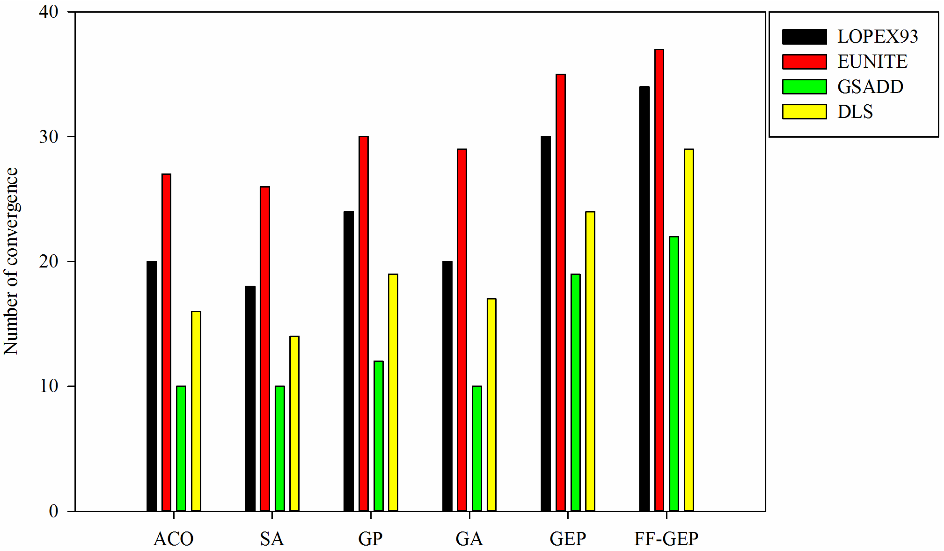
Figure 5. Comparison of number of convergence for ACO (Ant Colony Optimization), SA(Simulated Annealing), genetic programming (GP), genetic algorithm (GA), gene expression programming (GEP) and function finding algorithm using gene expression programming (FF-GEP).

Figure 5. Comparison of number of convergence for ACO (Ant Colony Optimization), SA(Simulated Annealing), genetic programming (GP), genetic algorithm (GA), gene expression programming (GEP) and function finding algorithm using gene expression programming (FF-GEP).

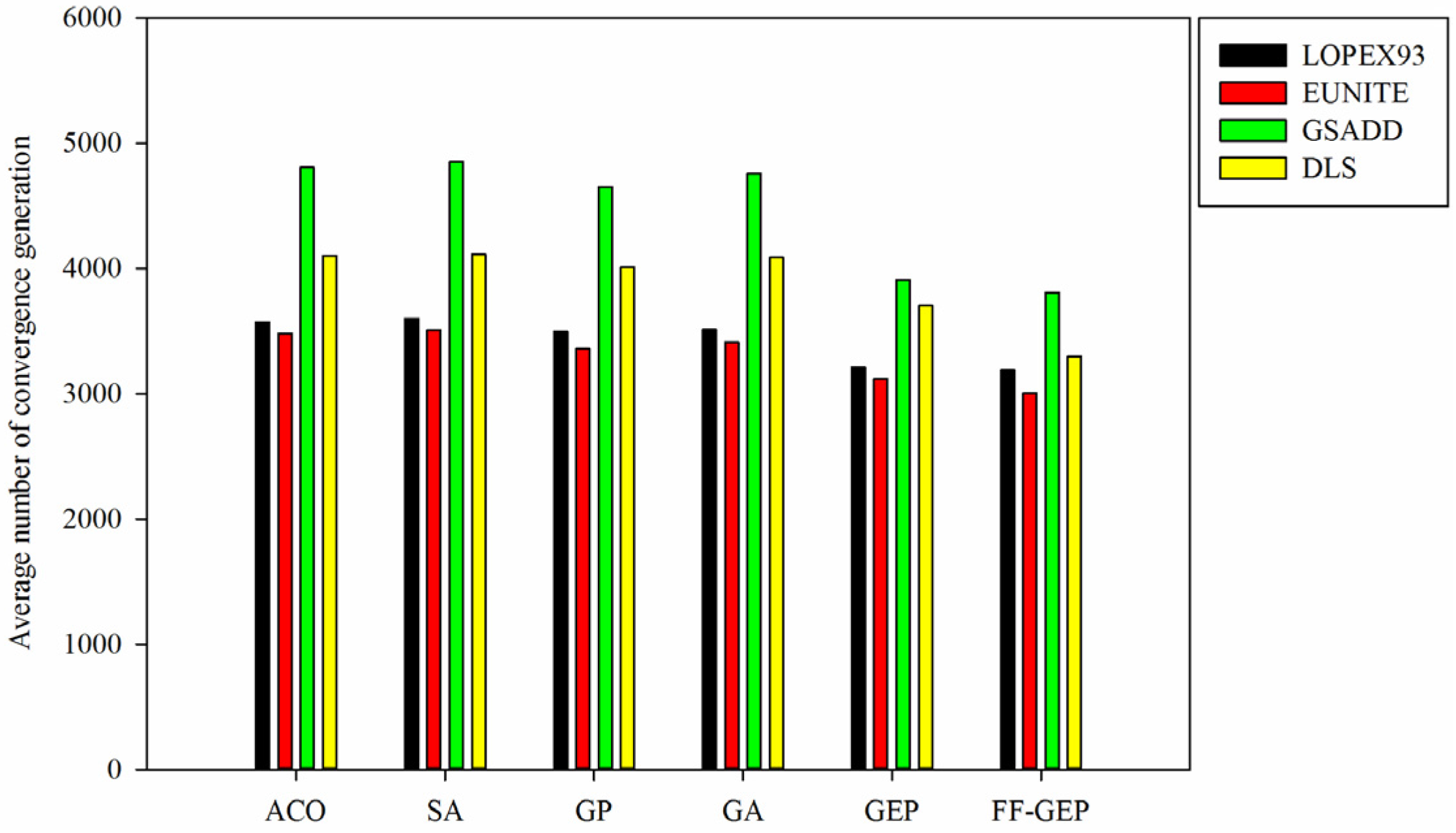
Figure 6. Comparison of average number of convergence generation for ACO (Ant Colony Optimization), SA(Simulated Annealing), genetic programming (GP), genetic algorithm (GA), gene expression programming (GEP) and function finding algorithm using gene expression programming (FF-GEP).

Figure 6. Comparison of average number of convergence generation for ACO (Ant Colony Optimization), SA(Simulated Annealing), genetic programming (GP), genetic algorithm (GA), gene expression programming (GEP) and function finding algorithm using gene expression programming (FF-GEP).

Table 2. Comparison of value of $R^2$ for four test datasets based on ACO (Ant Colony Optimization), SA(Simulated Annealing), genetic programming (GP), genetic algorithm (GA), gene expression programming (GEP) and function finding algorithm using gene expression programming (FF-GEP).

Datasets	Algorithms
	ACO	SA	GP	GA	GEP	FF-GEP
LOPEX93	0.8355	0.8291	0.8700	0.8490	0.9118	0.9381
EUNITE	0.8914	0.8901	0.9187	0.8926	0.9263	0.9575
GSADD	0.7012	0.6997	0.7393	0.7035	0.8321	0.8686
DLS	0.7801	0.7729	0.7903	0.7844	0.88	0.9097

Table 2. Comparison of value of $R^2$ for four test datasets based on ACO (Ant Colony Optimization), SA(Simulated Annealing), genetic programming (GP), genetic algorithm (GA), gene expression programming (GEP) and function finding algorithm using gene expression programming (FF-GEP).

Datasets	Algorithms
	ACO	SA	GP	GA	GEP	FF-GEP
LOPEX93	0.8355	0.8291	0.8700	0.8490	0.9118	0.9381
EUNITE	0.8914	0.8901	0.9187	0.8926	0.9263	0.9575
GSADD	0.7012	0.6997	0.7393	0.7035	0.8321	0.8686
DLS	0.7801	0.7729	0.7903	0.7844	0.88	0.9097

From Figure 5, for LOPEX93, EUNITE, GSADD and DLS datasets, compared with ACO, SA, GP, GA and GEP, number of convergence for FF-GEP maximally increases by 47.06%, 29.73%, 54.55% and 51.72%. In Figure 6, it is shown that for LOPEX93, EUNITE, GSADD and DLS datasets, compared with ACO, SA, GP, GA and GEP, average number of convergence generation for FF-GEP drops by 11.44%, 14.31%, 21.53% and 19.82%. This is mainly because, in FF-GEP, adaptive population generation strategy based on collaborative evolution of sub-population is applied to dynamically increase population size and diversity of individual so as to improve the probability of the global optimal solution and convergence speed.

In Table 2, it is shown that for LOPEX93, EUNITE, GSADD and DLS datasets, compared with ACO, SA, GP, GA and GEP, value of $R^2$ based on FF-GEP increases by 11.62%, 7.04%, 19.45% and 15.04%, respectively; and by Definition 5, value of $R^2$ based on FF-GEP is 0.9381, 0.9575, 0.8686 and 0.9097, respectively. It means that function model for all test datasets based on FF-GEP is best and can fit sample data well. 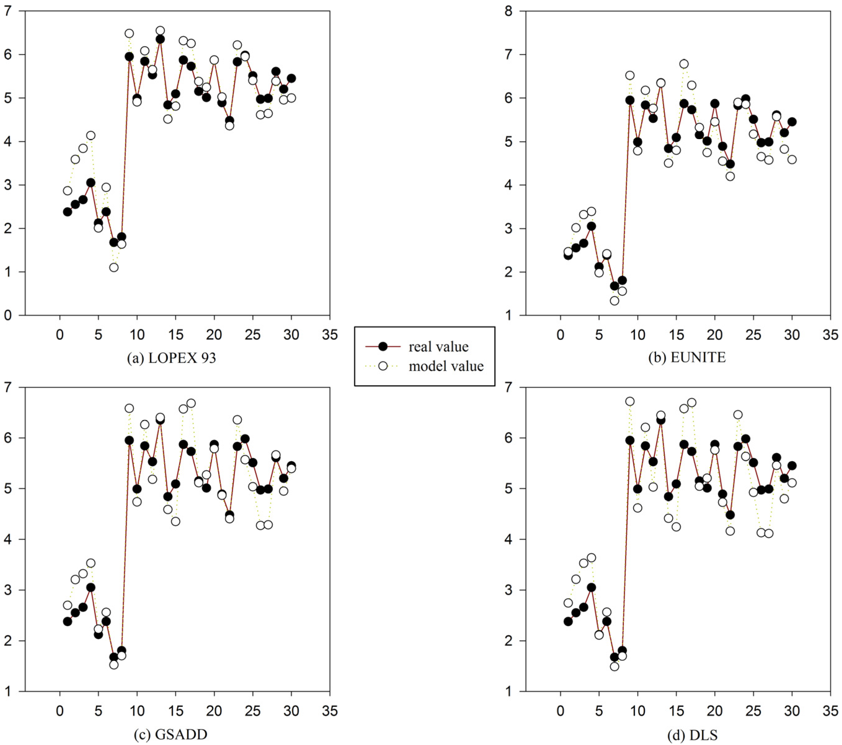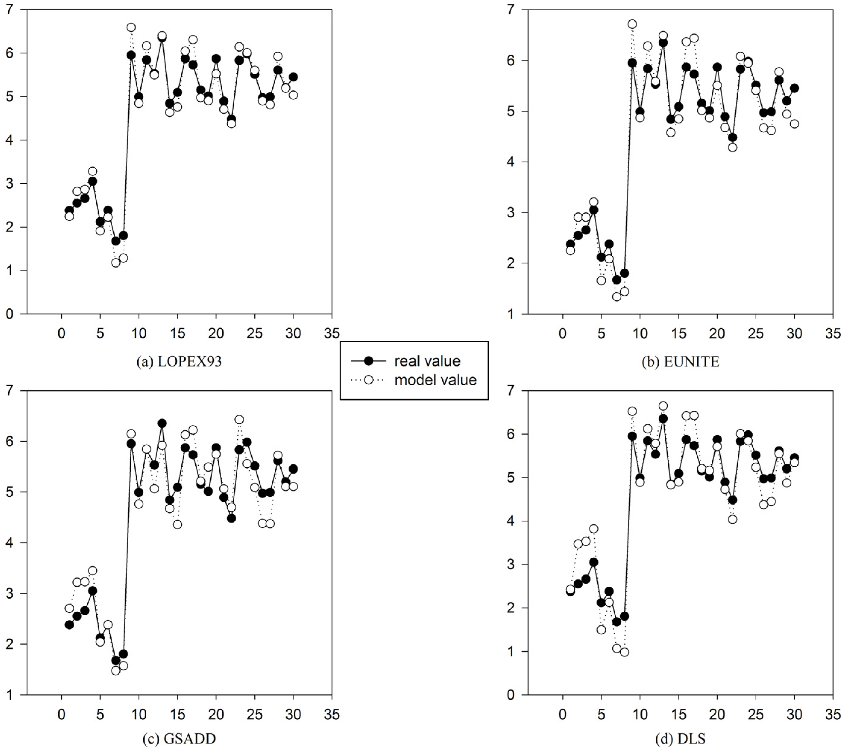From Figure 7, using FF-GEP, we can see that for LOPEX93, EUNITE, GSADD and DLS dataset, the maximum error between real value and model value is 1.1804, 0.9135, 0.9639 and 0.9515, respectively, and the minimum error is 0.0007, 0.0071, 0.0114 and 0.0251, respectively. It can be seen that the model has high prediction accuracy.

Example 2: In order to better evaluate performance of algorithm, Example 2 focuses on comparison of average time-consumption and fitting degree between real value and model value. Figure 8 shows average time-consumption of ACO, SA, GP, GA, GEP and FF-GEP. Average time-consumption of DGFMF-WSND with the increase of number of computing nodes is shown in Figure 9. Comparison of value of $R^2$ for LOPEX 93, EUNITE, GSADD and DLS datasets with the increase of number of computing nodes is shown in Figure 10. Figure 11 shows fitting degree between model value and real value of four test datasets in Table 1 based on DGFMF-WSND on six computing nodes.

Figure 7. Comparison between model value and real value of four test datasets in Table 1 using gene expression programming (GEP) and function finding algorithm using gene expression programming (FF-GEP). (a) Comparison between model value and real value of LOPEX93 datasets using GEP and FF-GEP; (b) comparison between model value and real value of EUNITE datasets using GEP and FF-GEP; (c) comparison between model value and real value of GSADD datasets using GEP and FF-GEP; and (d) comparison between model value and real value of DLS datasets using GEP and FF-GEP.

Figure 7. Comparison between model value and real value of four test datasets in Table 1 using gene expression programming (GEP) and function finding algorithm using gene expression programming (FF-GEP). (a) Comparison between model value and real value of LOPEX93 datasets using GEP and FF-GEP; (b) comparison between model value and real value of EUNITE datasets using GEP and FF-GEP; (c) comparison between model value and real value of GSADD datasets using GEP and FF-GEP; and (d) comparison between model value and real value of DLS datasets using GEP and FF-GEP.

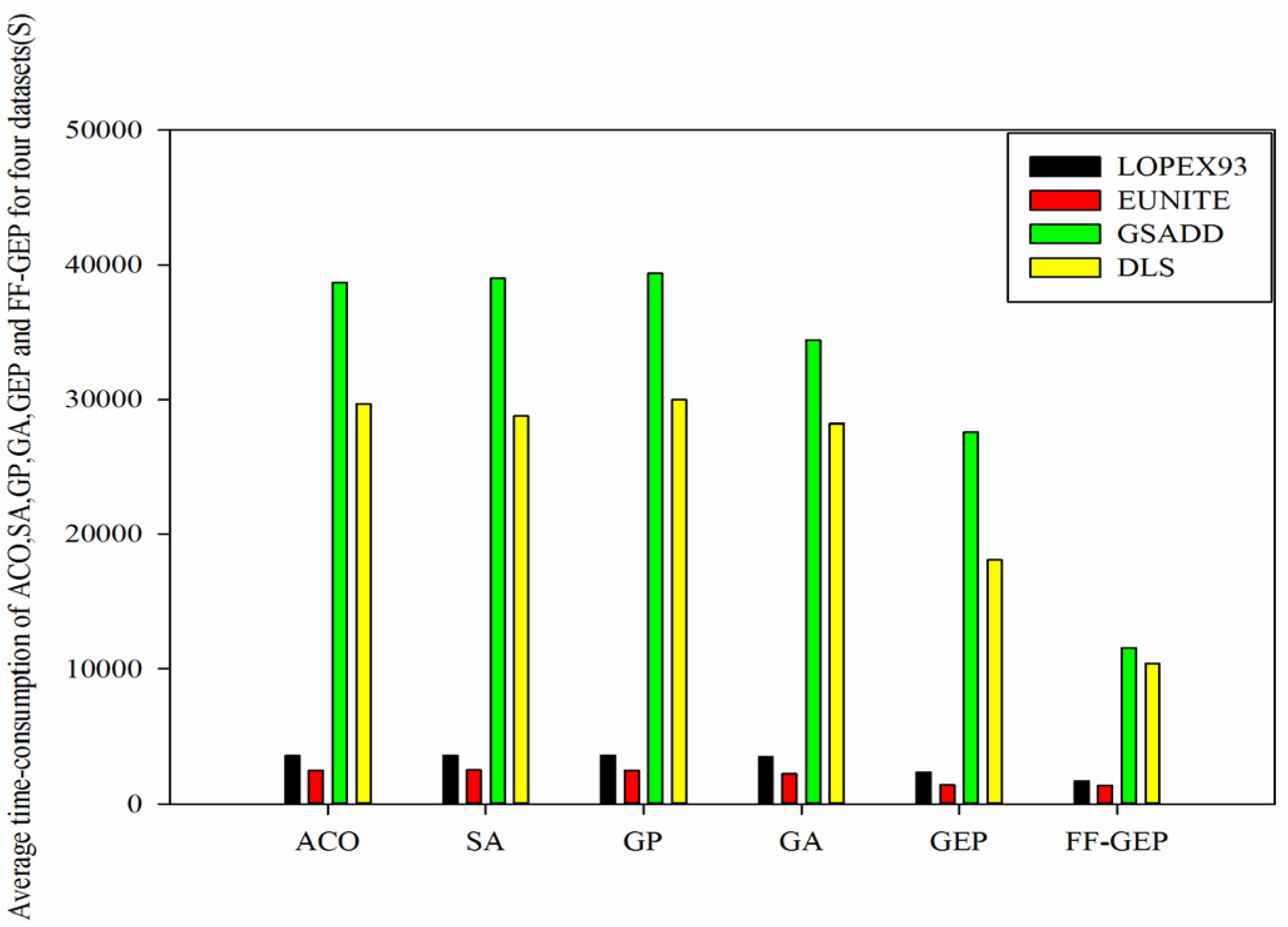
Figure 8. Comparison of average time-consumption of ACO (Ant Colony Optimization), SA(Simulated Annealing), genetic programming (GP), genetic algorithm (GA), gene expression programming (GEP) and function finding algorithm using gene expression programming (FF-GEP) for four datasets.

Figure 8. Comparison of average time-consumption of ACO (Ant Colony Optimization), SA(Simulated Annealing), genetic programming (GP), genetic algorithm (GA), gene expression programming (GEP) and function finding algorithm using gene expression programming (FF-GEP) for four datasets.

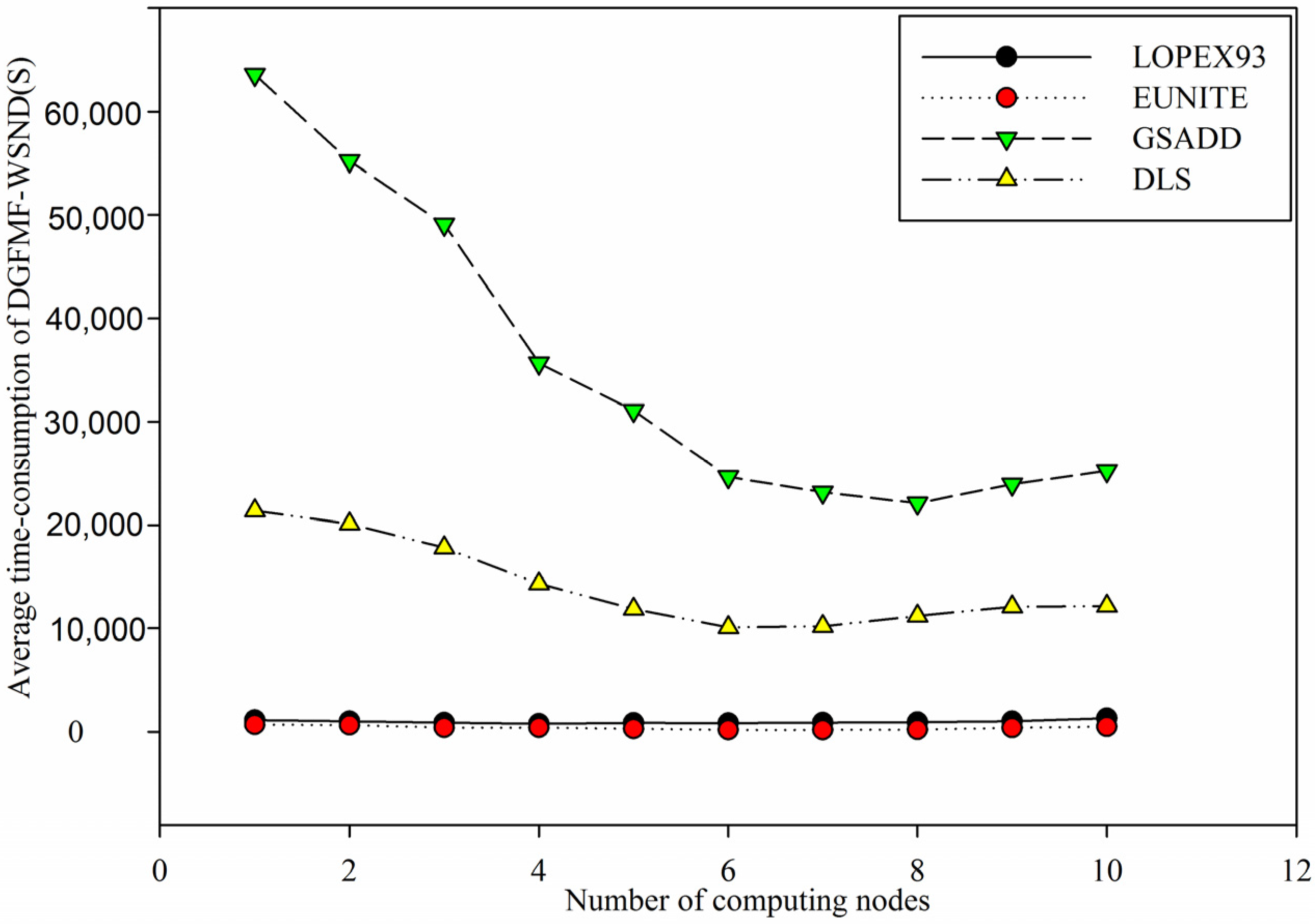
Figure 9. Comparison of average time-consumption of DGFMF-WSND for four datasets with the increase of number of computing nodes.

Figure 9. Comparison of average time-consumption of DGFMF-WSND for four datasets with the increase of number of computing nodes.

From Figure 8, we know that for LOPEX93, EUNITE, GSADD and DLS datasets, compared with ACO, average time-consumption of FF-GEP drops by 51.57%, 44.3%, 70.05% and 65.03%, respectively, compared with SA, average time-consumption of FF-GEP drops by 51.84%, 44.5%, 70.29% and 63.89%, respectively, and compared with GEP, average time-consumption of FF-GEP drops by 26.01%, 4.34%, 58.03% and 42.7%, respectively, in contrast to GP, decreases by 52.03%, 43.58%, 70.57% and 65.38%, respectively. While for LOPEX93, EUNITE, GSADD and DLS, average time-consumption of FF-GEP drops by 50.54%, 37.48%, 66.36% and 63.2% respectively in contrast to GA. This means that for LOPEX93, EUNITE, GSADD and DLS, FF-GEP outperforms all other algorithms on average time-consumption, followed by GEP. Especially, for GSADD dataset, average time-consumption of FF-GEP declines most quickly, and while, for EUNITE dataset, average time-consumption of FF-GEP declines most slowly. This is mainly because that compared with the other datasets, number of attributes of GSADD dataset is maximum, and number of attributes and instances of EUNITE dataset is minimum. Meanwhile, FF-GEP adopts adaptive population generation strategy based on collaborative evolution of sub-population to increase convergence speed. Figure 9 shows that with the increasing of number of computing nodes, average time-consumption of DGFMF-WSND drops gradually for LOPEX93, EUNITE, GSADD and DLS datasets. However, when number of computing nodes is increased from 7 to 10, average time-consumption of DGFMF-WSND will increase for all test datasets. This is mainly because that with the increasing of number of computing nodes, time of data transmission and global function generation will continue to increase so that total time-consumption of DGFMF-WSND will increase according to Equation (10). The decrease of time-consumption and the improvement of prediction accuracy of DGFMF-WSND will be helpful to find domain knowledge from massive and distributed wireless sensor network data.

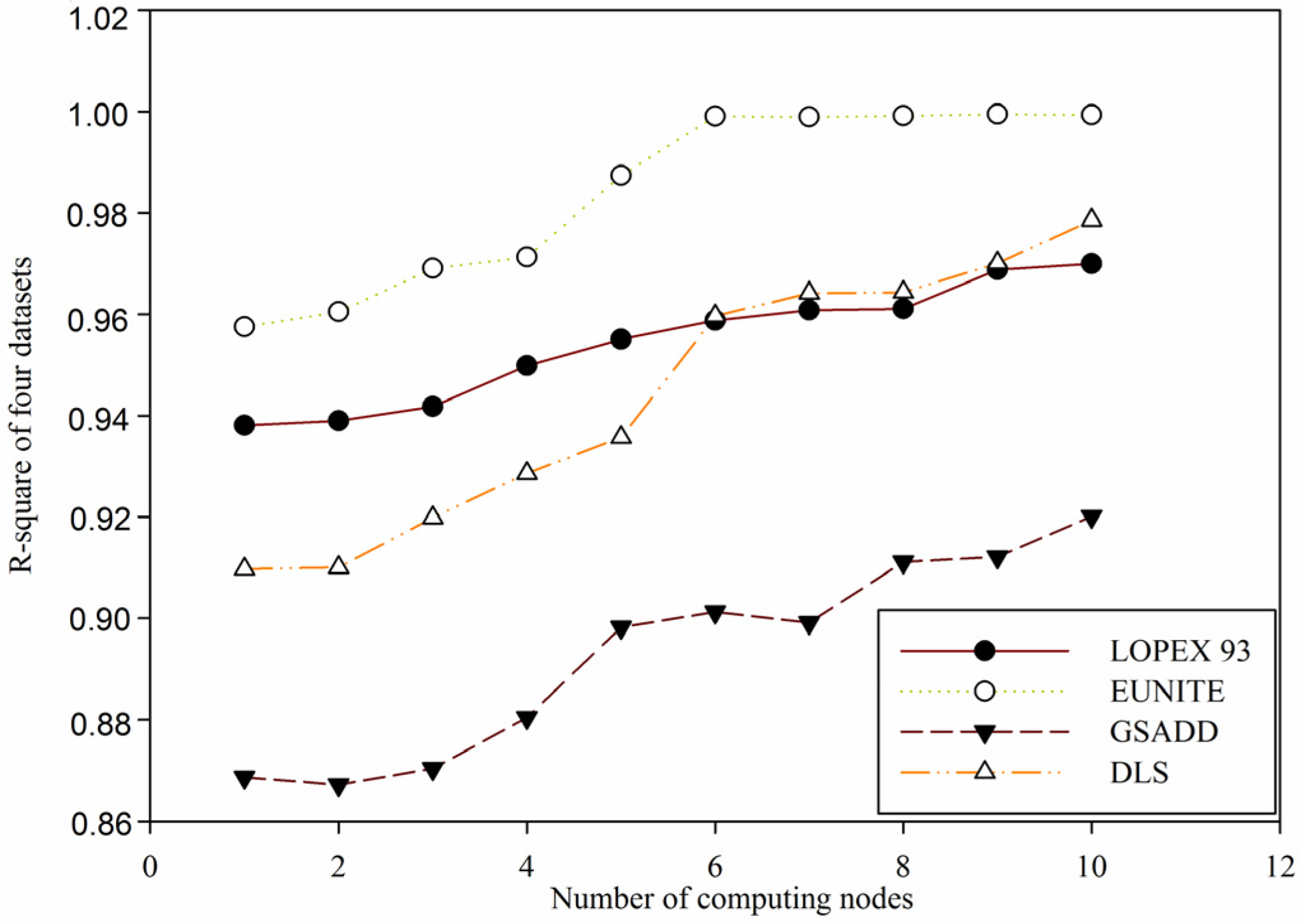
In Figure 10, it is shown that with the increasing of number of computing nodes, a value of $R^2$ for four datasets in Table 1 based on DGFMF-WSND increases gradually. According to Definition 5, we know that the bigger the value of $R^2$, the better the function model. When number of computing nodes is increased from 1 to 10, for LOPEX93, EUNITE, GSADD and DLS datasets, maximum value of $R^2$ is 0.97, 0.9994, 0.9201 and 0.9786, respectively. This means that with the increasing number of computing nodes, a global function model based on DGFMF-WSND can fit sample data well. From Figure 11, we can see that for LOPEX93, EUNITE, GSADD and DLS datasets, the maximum error between real value and model value is 0.7667, 0.6429, 0.915 and 0.7333, respectively, and the minimum error is 0.0359, 0.0106, 0.0107 and 0.0018, respectively. It can be seen that the global function model has high prediction accuracy.

Figure 10. Comparison of value of $R^2$ for four test datasets in Table 1 based on distributed global function model finding for wireless sensor networks data (DGFMF-WSND) with the increase of number of computing nodes.

Figure 10. Comparison of value of $R^2$ for four test datasets in Table 1 based on distributed global function model finding for wireless sensor networks data (DGFMF-WSND) with the increase of number of computing nodes.

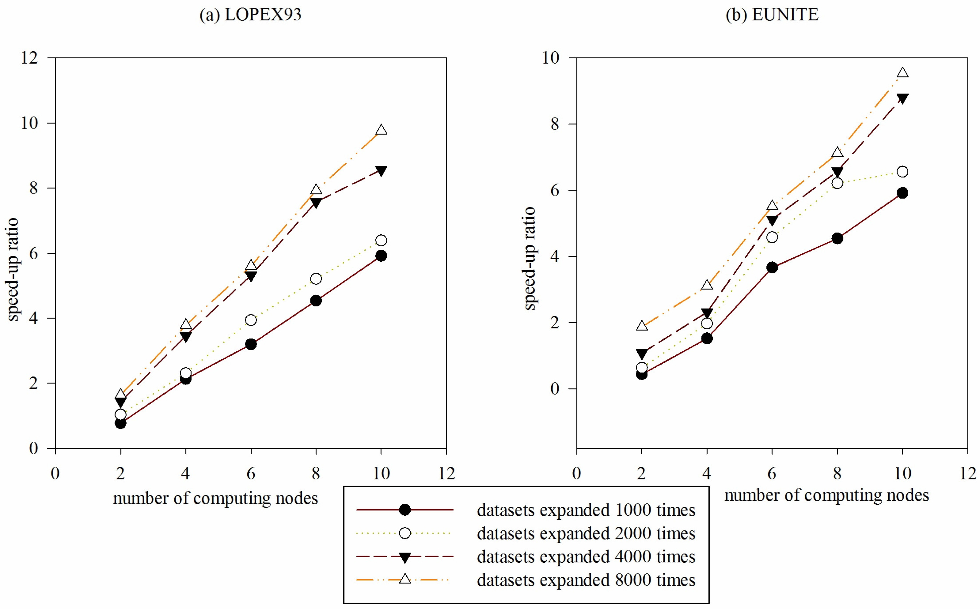
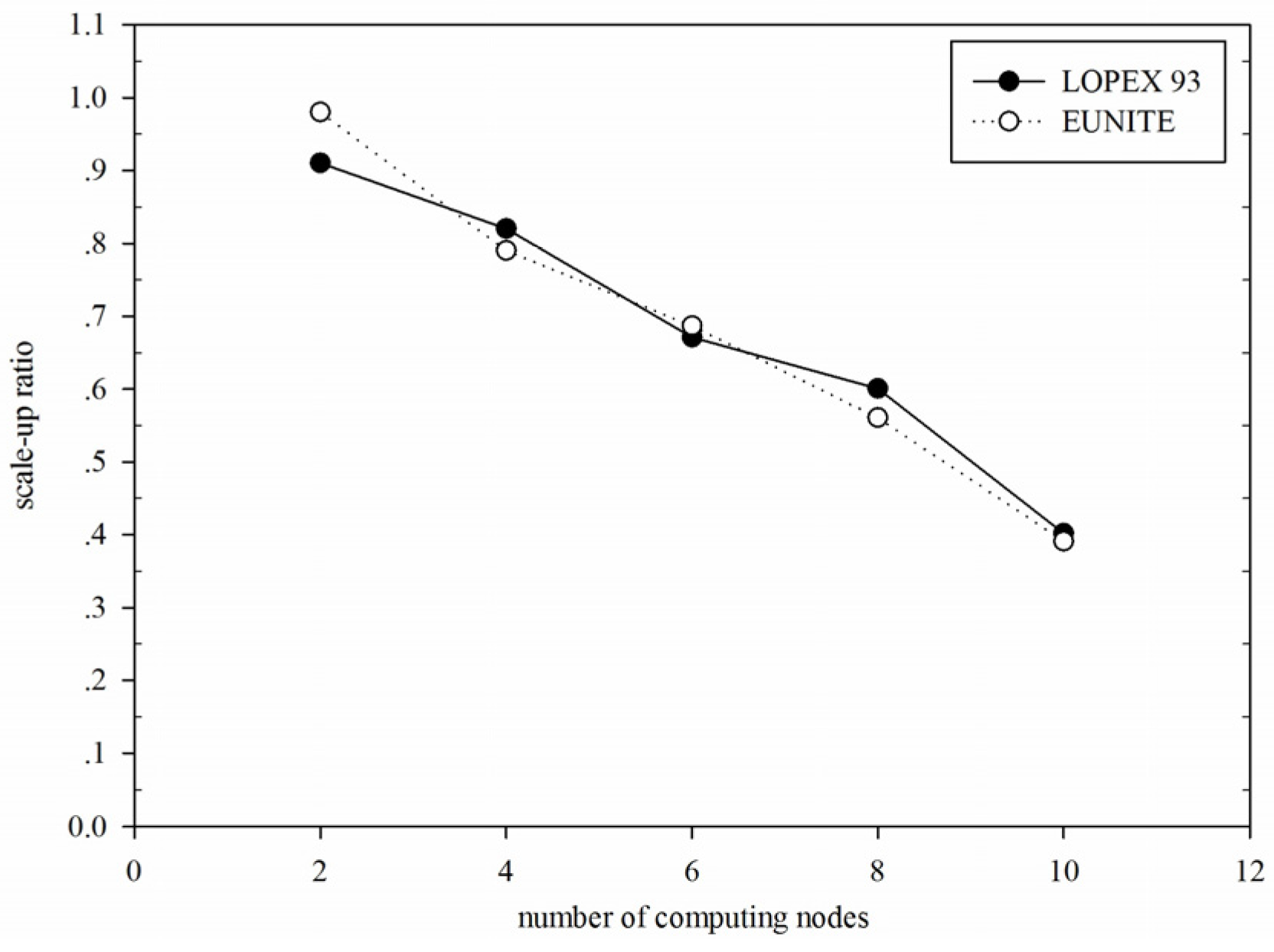
Example 3: To reflect the parallel performance of DGFMF-WSND, LOPEX93 and EUNITE datasets in Table 1 are expanded 1000, 2000, 4000 and 8000 times to respectively form four new datasets. Comparison of speed-up ratio of DGFMF-WSND for the four new datasets with the increase of number of computing nodes is shown in Figure 12. Figure 13 shows comparison of scale-up ratio of DGFMF-WSND for LOPEX93 and EUNITE datasets with the increase of number of computing nodes.

From Figure 12, with the increasing of number of computing nodes, speed-up ratio of DGFMF-WSND is increasing, and when size of the LOPEX93 and EUNITE dataset is expanded 8000 times, speed-up ratio of DGFMF-WSND is close to the linear increase. We know that change rate of speed-up ratio of an excellent parallel algorithm is close to 1. However, in concrete application, with the increasing of number of computing nodes, time-consumption of information transmission between node and node also increasing, linear speed-up ratio is very difficult to achieve. Figure 13 shows that for LOPEX93 and EUNITE, maximum scale-up ratio reaches 0.91 and 0.98, respectively; however, with the increasing of the number of computing nodes, scale-up ratio of DGFMF-WSND decreases gradually, while the slope of the decrease gets smaller. This means that the scalability of DGFMF-WSND is better.

Figure 11. Comparison between model value and real value of four test datasets in Table 1 based on DGFMF-WSND. (a) Comparison between model value and real value of LOPEX93 datasets based on DGFMF-WSND; (b) comparison between model value and real value of EUNITE datasets based on DGFMF-WSND ; (c) comparison between model value and real value of GSADD datasets based on DGFMF-WSND; and (d) comparison between model value and real value of DLS datasets based on DGFMF-WSND.

Figure 11. Comparison between model value and real value of four test datasets in Table 1 based on DGFMF-WSND. (a) Comparison between model value and real value of LOPEX93 datasets based on DGFMF-WSND; (b) comparison between model value and real value of EUNITE datasets based on DGFMF-WSND ; (c) comparison between model value and real value of GSADD datasets based on DGFMF-WSND; and (d) comparison between model value and real value of DLS datasets based on DGFMF-WSND.

Figure 12. Comparison of speed-up ratio of DGFMF-WSND for two datasets with the increase of number of computing nodes. (a) Comparison of speed-up ratio of DGFMF-WSND for LOPEX93 datasets with the increase of number of computing nodes; and (b) comparison of speed-up ratio of DGFMF-WSND for EUNITE datasets with the increase of number of computing nodes.

Figure 12. Comparison of speed-up ratio of DGFMF-WSND for two datasets with the increase of number of computing nodes. (a) Comparison of speed-up ratio of DGFMF-WSND for LOPEX93 datasets with the increase of number of computing nodes; and (b) comparison of speed-up ratio of DGFMF-WSND for EUNITE datasets with the increase of number of computing nodes.

Figure 13. Comparison of scale-up ratio of DGFMF-WSND for LOPEX93 and EUNITE datasets with the increase of number of computing nodes.

Figure 13. Comparison of scale-up ratio of DGFMF-WSND for LOPEX93 and EUNITE datasets with the increase of number of computing nodes.

7. Conclusions

With the development of wireless sensor networks, a large number of sensor data are collected. Finding a function model from the massive and distributed sensor data is very difficult. The requirement for the data mining techniques for wireless sensor network data led to the development of data mining algorithms. Each of the data mining algorithms solves certain problems of WSNs. Function mining is a significant part of data mining. With the quick increment of sensor nodes, a huge volume of dynamic, geographically distributed data are collected. How to efficiently analyze and transform this to usable knowledge by data mining is very important to the development and application of WSNs.

In order to better find a function model from massive and distributed sensor data, this paper proposes a function finding algorithm using gene expression programming (FF-GEP) with adaptive population generation strategy, and global model generation algorithm based on unconstrained nonlinear least squares (GMG-UNLS). On the basis of FF-GEP and GMG-UNLS, a distributed global function model finding for wireless sensor networks data (DGFMF-WSND) is present. In order to better evaluate performance of the proposed algorithm, in this paper, a grid computing platform based on WS-Core and four test datasets are provided. The experimental results show that compared with GA, GP and GEP, FF-GEP has an advantage in time-consumption, error of fitness and prediction accuracy, and DGFMF-WSND has lower time-consumption, higher degree of fitness and excellent speed-up ratio and scale-up ratio.

With the progress of sensor technology, applications for wireless sensor networks will become more mature and popular. All kinds of sensor data will become richer. Data mining techniques will be very important to execute in-depth analysis and improve performance of WSNs.