
Measurement Parameters Optimized for Sequential Multilateration in Calibrating a Machine Tool with a DOE Method

Abstract
:
1. Introduction
2. Calibration Setup Parameters of Multilateration Method
2.1. Machine Tool Setup Parameters
2.2. Tracking Laser Setup Parameters
2.3. Environment Setup Parameters
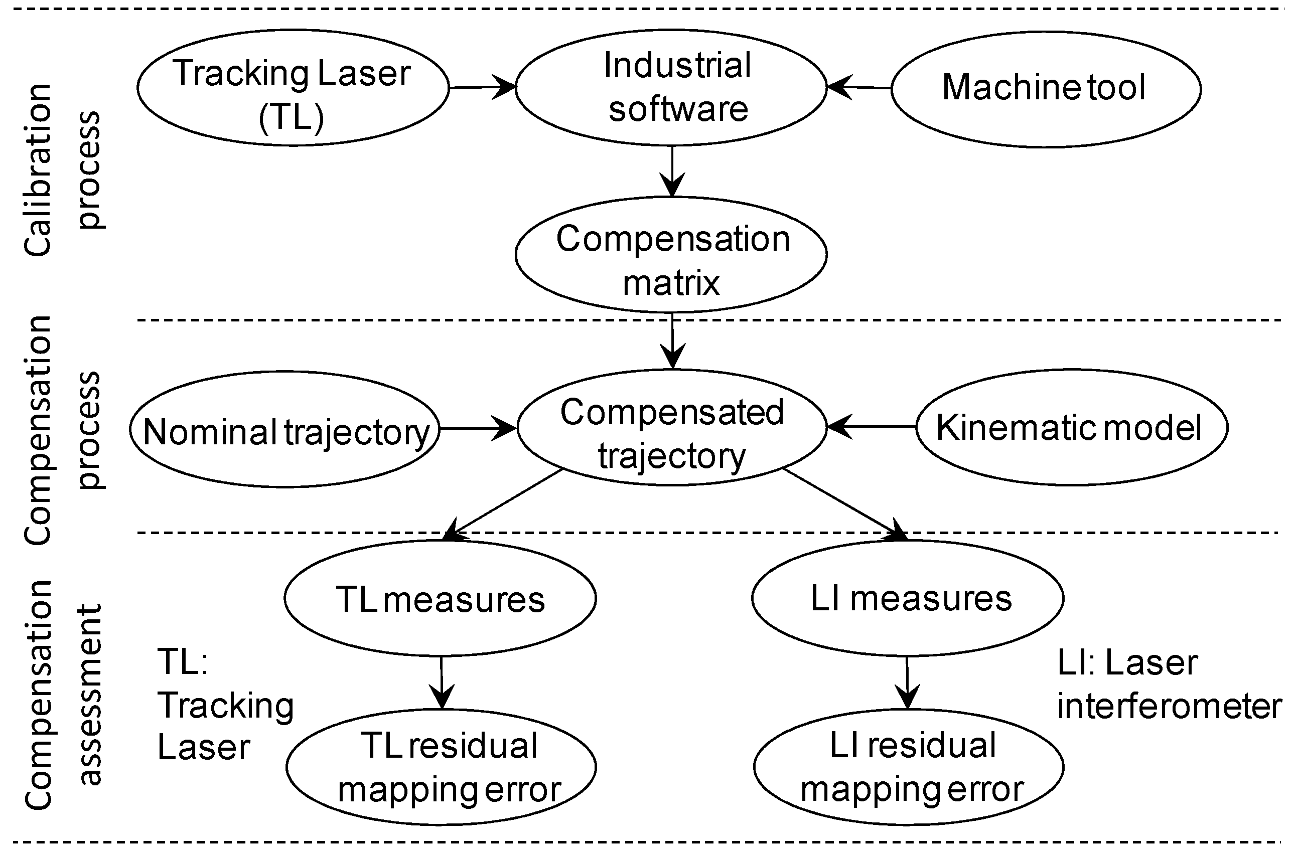
3. Machine Tool Compensation Assessment
3.1. Calibration Process
3.2. Compensation Process
3.3. Compensation Assessment
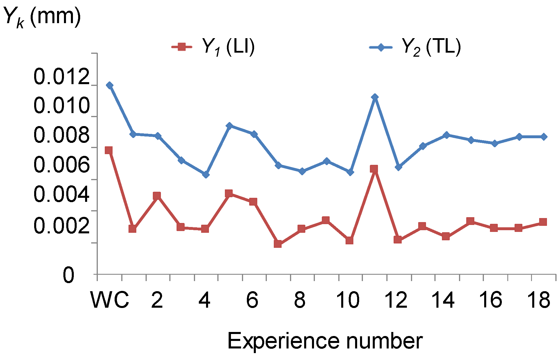
3.3.1. Laser Interferometer Measurements
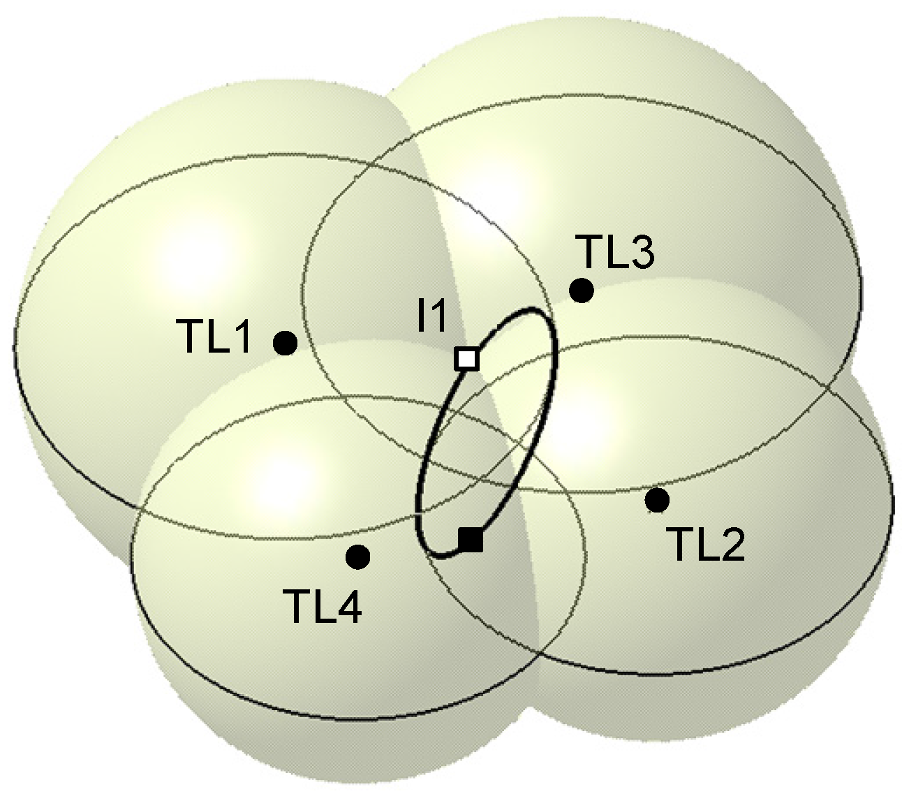
3.3.2. Sequential Multilateration Measurement Using a TL
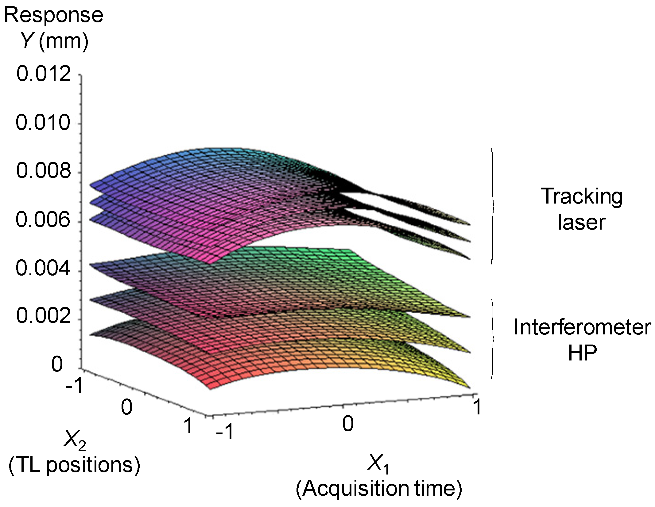
4. Optimization of the Calibration Setup Parameters
5. Discussion
6. Conclusions
Acknowledgments
Author Contributions
Conflicts of Interest
References
- Schwenke, H.; Knapp, W.; Haitjema, H.; Weckenmann, A.; Schmitt, R.; Delbressine, F. Geometric error measurement and compensation of machines-an update. CIRP Ann.-Manuf. Technol. 2008, 57, 660–675. [Google Scholar] [CrossRef]
- Díaz-Tena, E.; Ugalde, U.; De Lacalle, L.L.; De la Iglesia, A.; Calleja, A.; Campa, F.J. Propagation of assembly errors in multitasking machines by the homogenous matrix method. Int. J. Adv. Manuf. Technol. 2013, 68, 149–164. [Google Scholar] [CrossRef]
- Mian, N.S.; Fletcher, S.; Longstaff, A.P.; Myers, A. Efficient estimation by FEA of machine tool distortion due to environmental temperature perturbations. Precis. Eng. 2013, 37, 372–379. [Google Scholar] [CrossRef]
- Gomez-Acedo, E.; Olarra, A.; De Lacalle, L.L. A method for thermal characterization and modeling of large gantry-type machine tools. Int. J. Adv. Manuf. Technol. 2012, 62, 875–886. [Google Scholar] [CrossRef]
- Gebhardt, M.; Mayr, J.; Furrer, N.; Widmer, T.; Weikert, S.; Knapp, W. High precision grey-box model for compensation of thermal errors on five-axis. CIRP Ann.-Manuf. Technol. 2014, 63, 509–512. [Google Scholar] [CrossRef]
- Mayr, J.; Jedrzejewski, J.; Uhlmann, E.; Donmez, M.A.; Knapp, W.; Härtig, F.; Wendt, K.; Moriwaki, T.; Shore, P.; Schmitt, R.; et al. Thermal issues in machine tools. CIRP Ann.-Manuf. Technol. 2012, 61, 771–791. [Google Scholar] [CrossRef]
- Donmez, M.; Blomquist, D.S.; Hocken, R.J.; Liu, C.R.; Barash, M.M. A general methodology for machine tool accuracy enhancement by error compensation. Precis. Eng. 1986, 8, 187–196. [Google Scholar] [CrossRef]
- Archenti, A.; Nicolescu, N. Accuracy analysis of machine tools using Elastically Linked Systems. CIRP Ann.-Manuf. Technol. 2013, 62, 503–506. [Google Scholar] [CrossRef]
- Yuan, J.; Ni, J. The real-time error compensation technique for CNC machining systems. Mechatronics 1998, 8, 359–380. [Google Scholar] [CrossRef]
- Abbaszadeh-Mir, Y.; Mayer, J.R.R.; Cloutier, G.; Fortin, C. Theory and simulation for the identification of the link geometric errors for a five-axis machine tool using a telescoping magnetic ball-bar. Int. J. Prod. Res. 2002, 40, 4781–4797. [Google Scholar] [CrossRef]
- Lei, W.T.; Hsu, Y.Y. Error measurement of five-axis CNC machines with 3D probe–ball. J. Mater. Proc. Technol. 2003, 139, 127–133. [Google Scholar] [CrossRef]
- Weikert, S. R-Test, a New Device for Accuracy Measurements on Five Axis Machine Tools. CIRP Ann.-Manuf. Technol. 2004, 53, 429–432. [Google Scholar] [CrossRef]
- Castro, H.F.F.; Burdekin, M. Calibration system based on a laser interferometer for kinematic accuracy assessment on machine tools. Int. J. Mach. Tools Manuf. 2006, 46, 89–97. [Google Scholar] [CrossRef]
- Aguado, S.; Santolaria, J.; Samper, D.; Velázquez, J.; Javierre, C.; Fernández, Á. Adequacy of Technical and Commercial Alternatives Applied to Machine Tool Verification Using Laser Tracker. Appl. Sci. 2016, 6, 100. [Google Scholar] [CrossRef]
- Schneider, C.T. Lasertracer—A New Type of Self Tracking Laser Interferomete. In Proceedings of the 8th International Workshop on Accelerator Alignment, Geneva, Switzerland, 4–7 October 2004.
- Schwenke, H.; Franke, M.; Hannaford, J. Error mapping of CMMs and machine tools by a single tracking interferometer. CIRP Ann.-Manuf. Technol. 2005, 54, 475–478. [Google Scholar] [CrossRef]
- Lei, W.T.; Sung, M.P. NURBS-based fast geometric error compensation for CNC machine tools. Int. J. Mach. Tools Manuf. 2008, 48, 307–319. [Google Scholar] [CrossRef]
- Schwenke, H.; Schmitt, R.; Jatzkowski, P.; Warmann, C. On-the-fly calibration of linear and rotary axes of machine tools and CMMs using a tracking interferometer. CIRP Ann.-Manuf. Technol. 2009, 58, 477–480. [Google Scholar] [CrossRef]
- Linares, J.M.; Chaves-Jacob, J.; Schwenke, H.; Longstaff, A.; Fletcher, S.; Flore, J.; Wintering, J. Impact of measurement procedure when error mapping and compensating a small CNC machine using a multilateration laser interferometer. Precis. Eng. 2014, 38, 578–588. [Google Scholar] [CrossRef]


| Source | Parameter | Unit | Value |
|---|---|---|---|
| Machine tool | Warming cycle | - | Yes |
| Plate material | - | Steel | |
| Feedrate | mm/min | 1000 | |
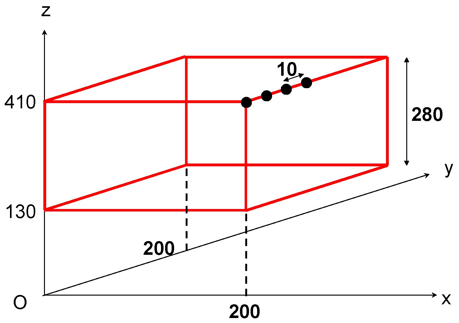
| Tracking laser | Type of pattern | - | Box |
| Sampling step | mm | 10 | |
| Acquisition time | s | Optimized | |
| Number of offsets | - | 4 | |
| Offset size | mm | Optimized | |
| Number of TL positions | - | Optimized | |
| Environment | Room temperature | °C | 20 |
| Experiments | X1 | X2 | X3 |
|---|---|---|---|
| 1 | −1 | −1 | −1 |
| 2 | 1 | −1 | −1 |
| 3 | −1 | 1 | −1 |
| 4 | 1 | 1 | −1 |
| 5 | −1 | −1 | 1 |
| 6 | 1 | −1 | 1 |
| 7 | −1 | 1 | 1 |
| 8 | 1 | −1 | −1 |
| 9 | −1 | 0 | 0 |
| 10 | 1 | 0 | 0 |
| 11 | 0 | −1 | 0 |
| 12 | 0 | 1 | 0 |
| 13 | 0 | 0 | −1 |
| 14 | 0 | 0 | −1 |
| 15 | 0 | 0 | 0 |
| 16 | 0 | 0 | 0 |
| 17 | 0 | 0 | 0 |
| 18 | 0 | 0 | 0 |
| Factors | DOE | |||
|---|---|---|---|---|
| Notation | Lower Value | Middle Value | Upper Value | |
| Acquisition time (s) | X1 | 0.5 | 1 | 1.5 |
| Number of TL positions | X2 | 4 | 5 | 6 |
| Offset size | X3 | Small | Medium | Large |
| Coefficient | Ŷ1 | Ŷ2 |
|---|---|---|
| 2.77 × 10⁻³ | 8.44 × 10⁻³ | |
| 1.17 × 10⁻⁴ | −2.63 × 10⁻⁴ | |
| −8.68 × 10⁻⁴ | −1.35 × 10⁻⁴ | |
| −7.02 × 10⁻⁴ | 1.21 × 10⁻⁴ | |
| −1.29 × 10⁻⁴ | −1.48 × 10⁻⁴ | |
| 1.23 × 10⁻³ | 7.17 × 10⁻⁴ | |
| −6.15 × 10⁻⁴ | 1.43 × 10⁻⁴ | |
| −4.38 × 10⁻⁴ | −7.29 × 10⁻⁵ | |
| 1.43 × 10⁻⁴ | 1.45 × 10⁻⁴ | |
| −1.89 × 10⁻⁴ | −9.5 × 10⁻⁴ |
| X1opt | X2opt | Yopt (μm) | Ywc (μm) |
|---|---|---|---|
| 1.5 | 6 | 5.99 | 12.2 |
© 2016 by the authors; licensee MDPI, Basel, Switzerland. This article is an open access article distributed under the terms and conditions of the Creative Commons Attribution (CC-BY) license (http://creativecommons.org/licenses/by/4.0/).
Share and Cite
Ezedine, F.; Linares, J.-M.; Chaves-Jacob, J.; Sprauel, J.-M. Measurement Parameters Optimized for Sequential Multilateration in Calibrating a Machine Tool with a DOE Method. Appl. Sci. 2016, 6, 313. https://doi.org/10.3390/app6110313
Ezedine F, Linares J-M, Chaves-Jacob J, Sprauel J-M. Measurement Parameters Optimized for Sequential Multilateration in Calibrating a Machine Tool with a DOE Method. Applied Sciences. 2016; 6(11):313. https://doi.org/10.3390/app6110313
Chicago/Turabian StyleEzedine, Fabien, Jean-Marc Linares, Julien Chaves-Jacob, and Jean-Michel Sprauel. 2016. "Measurement Parameters Optimized for Sequential Multilateration in Calibrating a Machine Tool with a DOE Method" Applied Sciences 6, no. 11: 313. https://doi.org/10.3390/app6110313
APA StyleEzedine, F., Linares, J.-M., Chaves-Jacob, J., & Sprauel, J.-M. (2016). Measurement Parameters Optimized for Sequential Multilateration in Calibrating a Machine Tool with a DOE Method. Applied Sciences, 6(11), 313. https://doi.org/10.3390/app6110313