Family of Quantum Sources for Improving Near Field Accuracy in Transducer Modeling by the Distributed Point Source Method

Abstract

The distributed point source method, or DPSM, developed in the last decade has been used for solving various engineering problems—such as elastic and electromagnetic wave propagation, electrostatic, and fluid flow problems. Based on a semi-analytical formulation, the DPSM solution is generally built by superimposing the point source solutions or Green’s functions. However, the DPSM solution can be also obtained by superimposing elemental solutions of volume sources having some source density called the equivalent source density (ESD). In earlier works mostly point sources were used. In this paper the DPSM formulation is modified to introduce a new kind of ESD, replacing the classical single point source by a family of point sources that are referred to as quantum sources. The proposed formulation with these quantum sources do not change the dimension of the global matrix to be inverted to solve the problem when compared with the classical point source-based DPSM formulation. To assess the performance of this new formulation, the ultrasonic field generated by a circular planer transducer was compared with the classical DPSM formulation and analytical solution. The results show a significant improvement in the near field computation.

1. Introduction

Modeling of ultrasonic and sonic fields generated by a planar transducer of finite dimension is a fundamental problem whose solution is available in textbooks in this area [1,2,3,4]. A good review of the earlier developments of the ultrasonic field modeling in front of a planar transducer can be found in [5]. A list of more recent developments is given by Sha et al. [6]. The pressure field in front of a planar transducer in a homogeneous isotropic fluid has been computed both in the time domain [5,7,8] and in the frequency domain [9,10,11,12,13,14]. In the frequency domain analysis, which is more popular, the transducers are assumed to be vibrating with constant amplitudes at certain frequencies, and the pressure fields in front of the transducers are computed. Most of these models give the steady state response of the transducers. Recently phased array transducers have been modeled as well [15,16,17,18,19,20].

In all modeling approaches that are based on the Huygens-Fresnel superposition principle and Rayleigh-Sommerfeld Integral (RSI) the strengths of the point sources modeling the transducer are assumed to be known. For type-I RSI the pressure distribution, and for type II RSI, the velocity distribution, on the transducer surfaces are assumed to be known. The distributed point source method (DPSM) [21,22,23] has been developed relatively recently for solving electrostatic, electromagnetic, and ultrasonic wave propagation problems. DPSM was first proposed by Placko and his co-workers for solving electrostatic and magnetostatic problems [21]. Later it was developed further by Placko and Kundu [22] and Kundu et al. [23] for solving ultrasonic problems. In ultrasonic modeling the source strengths can be treated as unknowns and obtained from the transducer surface boundary conditions as velocity or pressure. Alternately, all point sources can be assumed to have the same strength in order to model the uniform velocity condition at the transducer surface. In recent years DPSM has been extended to solve high frequency fluid flow problems [24] and fluid mechanics problems involving flow around an obstacle [25].

DPSM showed a significant savings in computational time compared to the Finite Elements Method (FEM) FEM technique for modeling ultrasonic problems [23,24,26] or electromagnetic problems [27]. A three-dimensional (3D) wave field modeling problem in a homogeneous fluid in front of a square transducer was solved in 2 min by DPSM while COMSOL Multi-Physics FEM code took 35 h to solve the identical problem on the same computer [23]. Jarvis and Cegla [26] used DPSM and FEM for solving ultrasonic wave reflections from a rough surface and concluded, “[FEM solution is] two orders of magnitude slower than the equivalent DPSM simulation on the same machine”.

In the above works on DPSM, point sources were uniformly distributed near the boundaries, interfaces, and front faces of the transducer (or emitter). The source strengths were then calculated by solving a system of linear equations that are obtained by satisfying boundary and continuity conditions for the problem geometry. In the near field, very close to the point sources, the computed field satisfies the boundary conditions only at the discrete points where the boundary conditions are specified. In between those points the boundary conditions are generally not satisfied. To overcome this shortcoming the use of a scaling factor was proposed [23]. In [23] Kundu et al. showed that the computed values in the far field (away from the transducer face) could be accurately modeled after incorporating the scaling factor. After considering this scaling factor for both near and far field computations, it was observed that at sections very close to the transducer face the average value of the computed field matched well with the true solution, although for individual points the deviation from the true solution could still be significant. To overcome this shortcoming Rahani and Kundu [28] tried DPSM with equivalent sources densities instead of the unique point source. They proposed two modifications—(1) G-DPSM or Gaussian DPSM replacing the single point source by a family of sources whose strength variations follow a Gaussian profile, and (2) ESM (Element Source Method): replacing discrete point sources by continuously varying element sources. Although these two modifications avoided the near field inaccuracy problem both approaches had their limitations. Results generated by G-DPSM were strongly affected by the Gaussian distribution function parameters and the ESM formulation was relatively complex. Thus, one major advantage of the DPSM formulation, its simplicity, was compromised by ESM. The concept of equivalent source density, including elemental point sources, linear, surface, or volume repartition, was presented and advocated by Placko et al. [29].

The objective of this paper is to propose a new ESD (equivalent source density) approach which is much simpler and can improve the near field computation accuracy without increasing the matrix size that is to be inverted for obtaining the solution. In this solution, the single point source is replaced by a source family. Point sources in a family are denoted as quantum sources to distinguish them from the regular point sources used in the classical DPSM formulation. A transducer can be modeled by M number of regular point sources in classical DPSM formulation or M × F quantum sources in the modified formulation. If every one of the M point sources are replaced by F number of quantum sources then the total number of quantum sources is equal to M × F. The quantum source strengths are set such that a given radiation pattern from the quantum source family is obtained.

G-DPSM, proposed by Rahani and Kundu [28], assumed a Gaussian distribution of source strength variations in a source family and their final results were strongly affected by the Gaussian distribution function parameters. However, in the technique proposed here, the strength variation of the quantum sources in a family is assumed to be unknown, but the radiation pattern generated by a source family is considered to follow a specific pattern—Gaussian distribution is one possibility, but not necessarily the only possibility. However, for not assuming a Gaussian distribution of the source strengths in a family significantly increases the number of unknown source strengths. It is illustrated in the Formulations section how this improvement can be achieved without increasing the final matrix size that is to be inverted. Thus, this modification can improve the computational accuracy without significantly increasing the computational time.

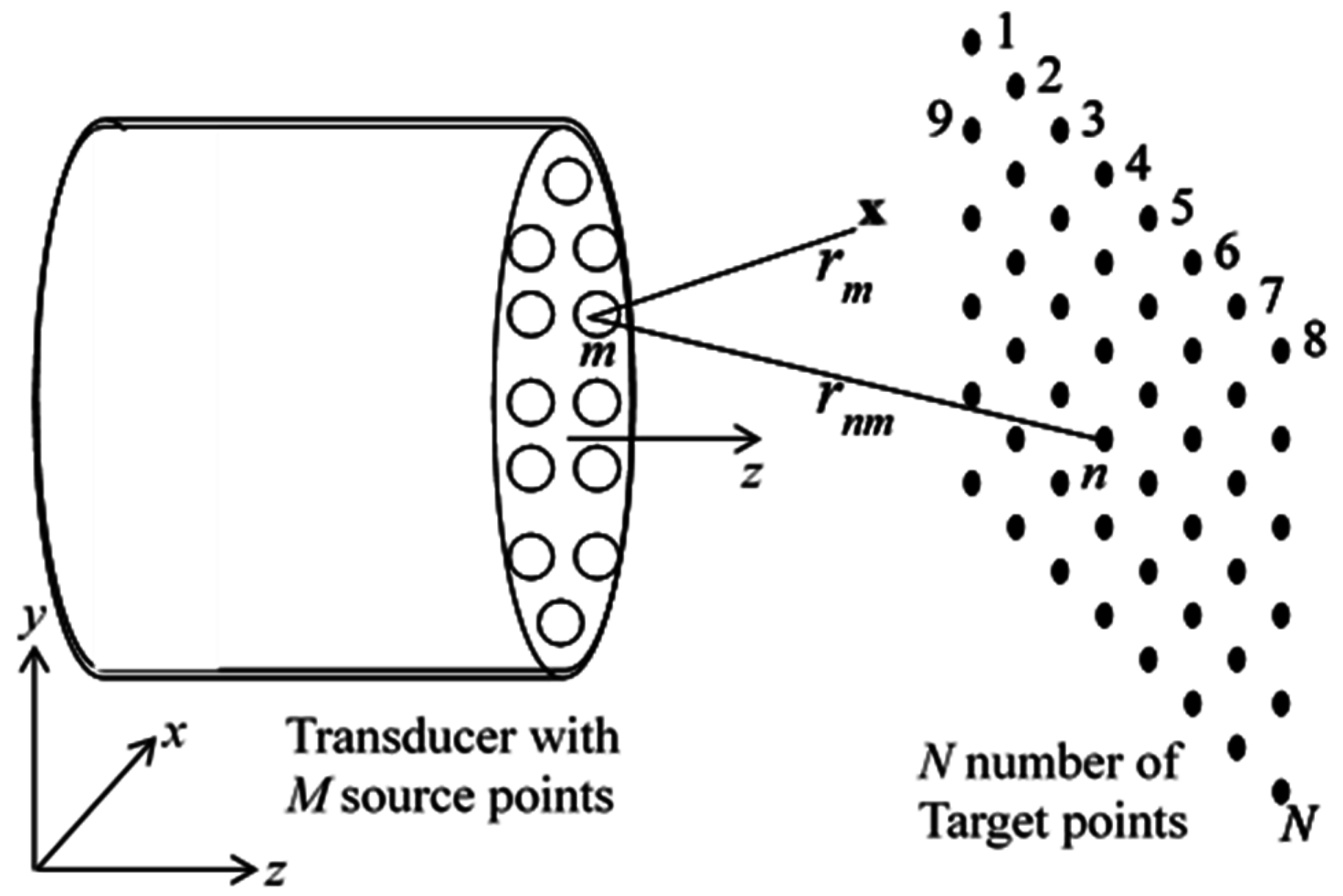
2. Formulations

The classical and the proposed DPSM formulations using family ESD are presented in this section. Although the classical DPSM formulation using unique point sources is available in the literature—in various publications mentioned above—for the benefit of the readers the basic steps of classical DPSM formulation and its current limitations are briefly reviewed first in the following subsection, before introducing the new formulation.

2.1. Classical DPSM Formulation: ESD is a Single Point Source

To generate the acoustic field in the fluid medium in front of an ultrasonic transducer or the electric field in front of an emitter by the DPSM technique, a number of point sources are placed slightly behind the transducer (or emitter) face as shown in Figure 1. This figure shows M number of source points placed at the centers of M spheres of radius r_s. Spheres touch the front face of the transducer. Thus, the point sources are located at a distance of r_s behind the transducer face to avoid the singularity. The DPSM formulation for ultrasonic wave field modeling is presented below. However, for electric field modeling the derivations are identical; the parameter names are simply changed from pressure, velocity, etc., to electric field, magnetic field, etc.

From [3] the pressure and velocity fields in a fluid at point x at a distance r_m from the m-th point source of strength Am can be written as:

The pressure field:

$$p_m(x)=p_m(r_m)=A_m\frac{\exp (i{k}_f{r}_m)}{r_m}$$

(1)

The velocity in the radial direction, at a distance r from the m-th point source:

$$v_m(r)=\frac{A_m}{i\mathsf{\omega }\mathsf{\rho }}\frac{\exp (i{k}_{f}r)}{r}\left(i{k}_f-\frac{1}{r}\right)$$

(2)

Therefore, the z-component of the velocity is:

$$v_{zm}(r)=\frac{A_m}{i\mathsf{\omega }\mathsf{\rho }}\frac{z\exp (i{k}_{f}r)}{r^2}\left(i{k}_f-\frac{1}{r}\right)$$

(3)

If there are M point sources distributed over the transducer surface, as shown in Figure 1, then the total pressure and the z-direction velocity values at point x are given by:

$$p(x)={\displaystyle \sum _{m=1}^M{p}_m(r_m)}={\displaystyle \sum _{m=1}^M{A}_m\frac{\exp (i{k}_f{r}_m)}{r_m}}$$

(4)

$$v_z={\displaystyle \sum }_{m=1}^M{v}_{zm}\left(r_m\right)={\displaystyle \sum }_{m=1}^M\frac{A_m}{i\mathsf{\omega }\mathsf{\rho }}\frac{z_m\exp \left(i{k}_f{r}_m\right)}{r_m^2}\left(i{k}_f-\frac{1}{r_m}\right)$$

(5)

where z_m is the distance of point x in the z-direction (perpendicular to the transducer face) measured from the m-th point source.

If the transducer surface velocity in the z direction is given by v₀ then for all x values on the transducer surface the velocity should be equal to v₀. Therefore:

$$v_z\left(x_{\mathrm{transducer}}\right)={\displaystyle \sum }_{m=1}^M\frac{A_m}{i\mathsf{\omega }\mathsf{\rho }}\frac{z_m\exp \left(i{k}_f{r}_m\right)}{r_m^2}\left(i{k}_f-\frac{1}{r_m}\right)=v_0$$

(6)

By satisfying Equation (6) at M points on the transducer surface, where the spheres touch the transducer face it is possible to obtain a system of M linear equations with M unknowns (A₁, A₂, A₃, …, A_m). If the point sources are placed slightly behind the transducer face as shown in Figure 1 then r_m of Equation (6) can never be equal to zero; thus, singular points are avoided.

If point x in Figure 1 coincides with the n-th target point and the velocity at the n-th target point or the observation point is to be computed then from Equation (6) one obtains:

$$v_z\left(x_n\right)={\displaystyle \sum }_{m=1}^M\frac{A_m}{i\mathsf{\omega }\mathsf{\rho }}\frac{z_{nm}\exp \left(i{k}_f{r}_{nm}\right)}{r_{nm}^2}\left(i{k}_f-\frac{1}{r_{nm}}\right)$$

(7)

In Equation (7) the first subscript n (of z and r) corresponds to the n-th target point and the second subscript m represents the m-th source point; therefore, $r_{nm}$ is the distance of the n-th target point from the m-th source point while $z_{nm}$ is the distance along the z-direction between the n-th target point and m-th source point. If the number of target points is made equal to the number of source points (both equal to M) and the target points are placed on the transducer surface then Equation (7) can be written in matrix form as:

$$V_S=M_{SS}{A}_S$$

(8)

where V_S is the (M × 1) vector of the velocity components at M number of target points on the transducer surface, and A_S is the (M × 1) vector containing the strengths of M number of point sources. M_SS is the (M × M) square matrix relating the two vectors V_S and A_S:

$${\left\{V_S\right\}}^T=\left[\begin{array}{ccc}{v}_{z1}& v_{z2} \dots & v_{zM}\end{array}\right]$$

(9)

where superscript T indicates the transpose and $v_{zm}$ represents the z-direction velocity at the m-th target point. If the transducer surface vibrates with a constant velocity amplitude v₀ then all elements of Equation (9) should have the same value v₀.

Vector A_S of the source strengths is given by:

$${\left\{A_S\right\}}^T=\left[\begin{array}{ccc}\begin{array}{ccc}{A}_1& A_2& A_3\end{array}& \dots & \begin{array}{ccc}{A}_{M-2}& A_{M-1}& A_M\end{array}\end{array}\right]$$

(10)

The matrix M_SS is obtained from Equation (7):

$$M_{SS}=\left[\begin{array}{cc}\begin{array}{c}\begin{array}{ccc}{m}_{11}& m_{12}& \dots \\ m_{21}& m_{22}& \dots \\ ⋮& ⋮& \ddots \end{array}\\ \begin{array}{ccc}{m}_{M1}& m_{M2}& \dots \end{array}\end{array}& \begin{array}{c}\begin{array}{c}{m}_{1M}\\ m_{2M}\\ ⋮\end{array}\\ m_{MM}\end{array}\end{array}\right]={\left[\begin{array}{ccc}f\left(z_{11},r_{11}\right)& f\left(z_{12},r_{12}\right)& \begin{array}{cc}\dots & f\left(z_{1M},r_{1M}\right)\end{array}\\ f\left(z_{21},r_{21}\right)& f\left(z_{22},r_{22}\right)& \begin{array}{cc}\dots & f\left(z_{2M},r_{2M}\right)\end{array}\\ \begin{array}{c}⋮\\ f\left(z_{M1},r_{M1}\right)\end{array}& \begin{array}{c}⋮\\ f\left(z_{M2},r_{M2}\right)\end{array}& \begin{array}{cc}\begin{array}{c}\ddots \\ \dots \end{array}& \begin{array}{c}⋮\\ f\left(z_{MM},r_{MM}\right)\end{array}\end{array}\end{array}\right]}_{M\times M}$$

(11)

where:

$$m_{nm}=f\left(z_{nm},r_{nm}\right)=\frac{z_{nm}\exp \left(i{k}_f{r}_{nm}\right)}{i\mathsf{\omega }\mathsf{\rho }·r_{nm}^2}\left(i{k}_f-\frac{1}{r_{nm}}\right)$$

(12)

Equation (8) can be inverted to obtain the point source strengths:

$$A_S={\left[M_{SS}\right]}^{-1}{V}_S$$

(13)

Instead of velocity, if pressure is specified on the transducer surface, then the source strength is obtained from the following equation:

$$A_S={\left[Q_{SS}\right]}^{-1}{P}_S$$

(14)

where P_S is the specified pressure field at the transducer surface and Q matrix relates the pressure field and the source strength (obtained from Equation (4)).

It should be noted here that Equation (13) can also be rewritten as $V_S^{*}=M_{SS}^{*}{A}_S^{*}$, where $V_S^{*}$ is a (3M × 1) vector containing all three components of velocity at M test points. For inversion of this equation, when needed, we may have used the concept of ESD, which are triplet sources used at every center point so that $A_S^{*}$ becomes a (3M × 1) vector containing all three strengths of the triplets at M source center points. See [3] for more detailed derivation.

After evaluating the source strength vector A_S from Equation (13) or (14) the pressure p(x) or velocity vector V(x) at any set of target points x (on the transducer surface or away) can be obtained from the following equations:

$$\begin{array}{l}{P}_T=Q_{TS}{A}_S\\ V_T=M_{TS}{A}_S\\ V_T^{*}=M_{TS}^{*}{A}_S\end{array}$$

(15)

For a set of N target points the vector P_T contains N pressure values at N target points, so its size is (N × 1). V_T is a (N × 1) vector containing z-components of velocity at N target points, and $V_T^{*}$ is a (3N × 1) vector containing all three components of velocity at N target points.

Therefore, the velocity field on the transducer surface can be computed at N number of points where N is much greater than M. It should be noted that only at M points the boundary conditions are specified. The velocity variation on the transducer face shown in Figure 2 is obtained with M = 464 (the number of source points considered for modeling the transducer) and N = 2500 (the number of target points where velocity is computed on the plane of the transducer face). Velocity values are computed on a square surface that coincides with the transducer face. Some points on the square surface that are near its four corners are outside the transducer face and give zero displacement, as expected. However, on the transducer face the computed velocity is not uniform. It reaches a peak value of v₀ (in our case 1) at 464 points where small spheres of Figure 1 touch the transducer face but, in between these points, they are significantly smaller. Thus, the average velocity of the transducer face becomes less than v₀ giving rise to smaller pressure values from the DPSM analysis. When the DPSM results are multiplied by an appropriate scaling factor (obtained by dividing the given transducer face velocity by the average velocity of the transducer surface) then the discrepancy in the far field disappears [3]. However, in the near field (on the transducer face and very close to the transducer face) the scaling factor multiplication cannot remove the oscillation patterns shown in Figure 2 although their average value matches with the prescribed velocity value of the transducer face.

2.2. Formulation with ESD Families

In the proposed formulation every point source of Figure 1 is replaced by a family of point sources as shown in Figure 3. These point sources in the family are called quantum sources to distinguish them from the unique point sources in the classical DPSM formulation. If there are F number of quantum sources in every family then, from M number of original point sources, a total of (M × F) quantum sources are generated. If classical DPSM formulation as described above is applied to these (M × F) quantum sources then the matrix size becomes (M × F) × (M × F) (see Equations (13) and (14)).

To reduce the matrix size and the number of unknown source strengths from (M × F) to M it is assumed that the relative source strength distribution within a family is the same for all M families. Then, F sources of the i-th family (i = 1, 2, …, M) should have the following source strength distribution:

$$A_i={\mathsf{\lambda }}_{i}q={\lambda }_i{\left[\begin{array}{ccc}{q}_1& q_2& q_3\end{array}\begin{array}{ccc} \cdots & q_{\left(F-1\right)}& q_F\end{array}\right]}^T$$

(16)

The i-th family strength is denoted by ${\mathsf{\lambda }}_i$ and its distribution is denoted by the vector q. The distribution vector q is the same for all M families but the strength ${\mathsf{\lambda }}_i$ can be different for different families. Then the velocity field at M target points generated by (M × F) quantum sources can be written as:

$$\left\{\begin{array}{c}\begin{array}{c}{v}_{z1}\\ v_{z2}\\ v_{z3}\end{array}\\ ⋮\\ v_{zM}\end{array}\right\}=\left[\begin{array}{cccc}\left(\begin{array}{ccc}{m}_{11}^1& \dots & m_{1F}^1\end{array}\right)& \left(\begin{array}{ccc}{m}_{11}^2& \dots & m_{1F}^2\end{array}\right)& \dots & \left(\begin{array}{ccc}{m}_{11}^M& \dots & m_{1F}^M\end{array}\right)\\ \left(\begin{array}{ccc}{m}_{21}^1& \dots & m_{2F}^1\end{array}\right)& \left(\begin{array}{ccc}{m}_{21}^2& \dots & m_{2F}^2\end{array}\right)& \dots & \left(\begin{array}{ccc}{m}_{21}^M& \dots & m_{2F}^M\end{array}\right)\\ \left(\begin{array}{ccc}{m}_{31}^1& \dots & m_{3F}^1\end{array}\right)& \left(\begin{array}{ccc}{m}_{31}^2& \dots & m_{3F}^2\end{array}\right)& \dots & \left(\begin{array}{ccc}{m}_{31}^M& \dots & m_{3F}^M\end{array}\right)\\ & ⋮\hfill & & ⋮\\ \left(\begin{array}{ccc}{m}_{M1}^1& \dots & m_{MF}^1\end{array}\right)& \left(\begin{array}{ccc}{m}_{M1}^2& \dots & m_{MF}^2\end{array}\right)& \dots & \left(\begin{array}{ccc}{m}_{M1}^M& \dots & m_{MF}^M\end{array}\right)\end{array}\right]\left\{\begin{array}{c}\begin{array}{c}{\mathsf{\lambda }}_1\left(\begin{array}{c}{q}_1\\ ⋮\\ q_F\end{array}\right)\\ {\mathsf{\lambda }}_2\left(\begin{array}{c}{q}_1\\ ⋮\\ q_F\end{array}\right)\\ ⋮\end{array}\\ ⋮\\ {\mathsf{\lambda }}_M\left(\begin{array}{c}{q}_1\\ ⋮\\ q_F\end{array}\right)\end{array}\right\}$$

(17)

where $m_{jk}^i$ represents the velocity at the i-th target point generated by the k-th quantum source of unit amplitude at the j-th family. The above equation can be re-written as:

$$\left\{\begin{array}{c}\begin{array}{c}{v}_{z1}\\ v_{z2}\\ v_{z3}\end{array}\\ ⋮\\ v_{zM}\end{array}\right\}=\left[\begin{array}{cccc}\left(\begin{array}{ccc}{m}_{11}^1& \dots & m_{1F}^1\end{array}\right)\left(\begin{array}{c}{q}_1\\ ⋮\\ q_F\end{array}\right)& \left(\begin{array}{ccc}{m}_{11}^2& \dots & m_{1F}^2\end{array}\right)\left(\begin{array}{c}{q}_1\\ ⋮\\ q_F\end{array}\right)& \dots & \left(\begin{array}{ccc}{m}_{11}^M& \dots & m_{1F}^M\end{array}\right)\left(\begin{array}{c}{q}_1\\ ⋮\\ q_F\end{array}\right)\\ \left(\begin{array}{ccc}{m}_{21}^1& \dots & m_{2F}^1\end{array}\right)\left(\begin{array}{c}{q}_1\\ ⋮\\ q_F\end{array}\right)& \left(\begin{array}{ccc}{m}_{21}^2& \dots & m_{2F}^2\end{array}\right)\left(\begin{array}{c}{q}_1\\ ⋮\\ q_F\end{array}\right)& \dots & \left(\begin{array}{ccc}{m}_{21}^M& \dots & m_{2F}^M\end{array}\right)\left(\begin{array}{c}{q}_1\\ ⋮\\ q_F\end{array}\right)\\ \left(\begin{array}{ccc}{m}_{31}^1& \dots & m_{3F}^1\end{array}\right)\left(\begin{array}{c}{q}_1\\ ⋮\\ q_F\end{array}\right)& \left(\begin{array}{ccc}{m}_{31}^2& \dots & m_{3F}^2\end{array}\right)\left(\begin{array}{c}{q}_1\\ ⋮\\ q_F\end{array}\right)& \dots & \left(\begin{array}{ccc}{m}_{31}^M& \dots & m_{3F}^M\end{array}\right)\left(\begin{array}{c}{q}_1\\ ⋮\\ q_F\end{array}\right)\\ & ⋮\hfill & & ⋮\\ \left(\begin{array}{ccc}{m}_{M1}^1& \dots & m_{MF}^1\end{array}\right)\left(\begin{array}{c}{q}_1\\ ⋮\\ q_F\end{array}\right)& \left(\begin{array}{ccc}{m}_{M1}^2& \dots & m_{MF}^2\end{array}\right)\left(\begin{array}{c}{q}_1\\ ⋮\\ q_F\end{array}\right)& \dots & \left(\begin{array}{ccc}{m}_{M1}^M& \dots & m_{MF}^M\end{array}\right)\left(\begin{array}{c}{q}_1\\ ⋮\\ q_F\end{array}\right)\end{array}\right]\left\{\begin{array}{c}{\mathsf{\lambda }}_1\\ {\mathsf{\lambda }}_2\\ ⋮\\ {\mathsf{\lambda }}_M\end{array}\right\}$$

(18)

Or:

$$\left\{\begin{array}{c}\begin{array}{c}{v}_{z1}\\ v_{z2}\\ v_{z3}\end{array}\\ ⋮\\ v_{zM}\end{array}\right\}=\left[\begin{array}{cc}\begin{array}{c}\begin{array}{c}\begin{array}{ccc}{M}_{11}& M_{12}& \dots \\ M_{21}& M_{22}& \dots \\ M_{31}& M_{32}& \dots \end{array}\\ ⋮ \end{array}\\ \begin{array}{ccc}{M}_{M1}& M_{M2}& \dots \end{array}\end{array}& \begin{array}{c}\begin{array}{c}\begin{array}{c}{M}_{1M}\\ M_{2M}\\ M_{3M}\end{array}\\ ⋮\end{array}\\ M_{MM}\end{array}\end{array}\right]\left\{\begin{array}{c}\begin{array}{c}{\mathsf{\lambda }}_1\\ {\mathsf{\lambda }}_2\\ ⋮\end{array}\\ ⋮\\ {\mathsf{\lambda }}_M\end{array}\right\}$$

(19)

Therefore:

$$\left\{\begin{array}{c}\begin{array}{c}{\mathsf{\lambda }}_1\\ {\mathsf{\lambda }}_2\\ ⋮\end{array}\\ ⋮\\ {\mathsf{\lambda }}_M\end{array}\right\}={\left[\begin{array}{cc}\begin{array}{c}\begin{array}{c}\begin{array}{ccc}{M}_{11}& M_{12}& \dots \\ M_{21}& M_{22}& \dots \\ M_{31}& M_{32}& \dots \end{array}\\ ⋮ \end{array}\\ \begin{array}{ccc}{M}_{M1}& M_{M2}& \dots \end{array}\end{array}& \begin{array}{c}\begin{array}{c}\begin{array}{c}{M}_{1M}\\ M_{2M}\\ M_{3M}\end{array}\\ ⋮\end{array}\\ M_{MM}\end{array}\end{array}\right]}^{-1}\left\{\begin{array}{c}\begin{array}{c}{v}_{z1}\\ v_{z2}\\ v_{z3}\end{array}\\ ⋮\\ v_{zM}\end{array}\right\}$$

(20)

It should be noted that both Equations (13) and (20) require inversion of the M × M matrix. However, for classical DPSM formulation (Equation (13)) the number of point sources is M while for the new formulation (Equation (20)) the number of quantum sources is (M × F).

To obtain the relative strength variation vector $q={\left[\begin{array}{ccc}{q}_1& q_2& q_3\end{array}\begin{array}{ccc}\cdots & q_{\left(F-1\right)}& q_F\end{array}\right]}^T$ (see Equation (16)) of the quantum sources in a family the radiation pattern generated by the quantum sources will have to be assumed. The radiation pattern describes the velocity or pressure distribution generated by a family of quantum sources for ultrasonic field modeling, or electric field distribution for electrostatic problems.

In the classical DPSM formulation Green’s function for a point source determines the radiation pattern. Typically the wavefront generated by a point source is a sphere in an isotropic medium. However, for a family of quantum sources any radiation pattern can be achieved by properly adjusting the source strength distribution vector q in the family. We may notice that, for the far field, all of the terms of the line matrix $\left(\begin{array}{ccc}{m}_{11}^1& \dots & m_{1F}^1\end{array}\right)$ of Equation (18) tends to the same value, which corresponds to the $m_{11}$ term of Equation (12). Then, the family is seen as a cluster of sources equivalent to a unique point source of strength equal to the sum of $\left[\begin{array}{ccc}{q}_1& q_2& q_3\end{array}\begin{array}{ccc}\cdots & q_{\left(F-1\right)}& q_F\end{array}\right]$.

3. Results

Numerical results are generated for a Gaussian radiation pattern, as shown in Figure 4, generated by every family. Quantum source strengths within every family are obtained for this radiation pattern following the classical DPSM approach and ignoring the presence of other families. Then the pressure field in the fluid in front of the uniformly vibrating circular transducer with a radius of 6 mm is computed by considering all families, as shown in Figure 3. For clarity, 50 families are shown in Figure 3. However, during actual computation 464 families were considered. Every family is composed of 30 quantum sources. The transducer vibration frequency is 1 MHz. Fluid properties considered for this simulation are those of water—density (ρ) = 1000 kg/m³ and P-wave speed (c_f) = 1480 m/s.

The normal velocity component is first computed at 2500 points on a square surface that coincides with the transducer surface. The computed results with the new formulation is shown in Figure 5a and with the old formulation (classical DPSM) is shown in Figure 5b. Clearly, the oscillations are much less (almost disappearing) in Figure 5a. In both formulations the final matrix that was inverted had dimensions of 464 × 464. In the new formulation 464 clusters gave this matrix dimension, while in the old formulation 464 point sources generated this matrix. To improve the accuracy of the classical DPSM computation, the number of point sources and, hence, the matrix dimension must be increased while, in the new formulation, the number of quantum sources can be increased without increasing the number of clusters and, therefore, the matrix dimension.

Figure 6 shows the variation of the normal velocity along the diameter (y-axis going through the center of the transducer face). The continuous line shows the field computed by the new formulation while the dotted line is obtained from the classical DPSM formulation. Nine points where the two curves match correspond to the boundary points where the velocity is specified. These nine points out of 464 points appear on the diameter along which the velocity values are computed. Classical DPSM gives correct values only at those nine points and deviates significantly from the correct value of 1 at other points. The results generated by the new formulation are much closer to the true values and match with the true values at several other points where the boundary conditions are not specified. To get a quantitative measure of the difference between these curves the error is computed using the following equation:

$$\mathrm{Error}=100\times \sqrt{\frac{{{\displaystyle \sum }}_i{\left\{V{\left(i\right)}_{\mathrm{true}}-V{\left(i\right)}_{\mathrm{computed}}\right\}}^2}{{{\displaystyle \sum }}_{i}V{\left(i\right)}_{\mathrm{true}}^2}}$$

(21)

where V(i)_true is the true value of the velocity amplitude at the i-th point, which is 1 on the transducer surface and zero outside the transducer, as shown in Figure 6. The true value is denoted as the objective function (dashed-dotted line) in this figure. V(i)_computed are the computed values (continuous and dotted lines of Figure 6). The computed error is 34.8% for classical DPSM and 3.05% for proposed DPSM with the family ESD technique.

From the symmetry of the problem it is obvious that the fluid velocity parallel to the transducer surface in the x-direction should be zero along the y-axis going through the transducer center. This velocity component on the transducer surface is plotted in Figure 7. It is close to zero for the new formulation. However, for the classical formulation, strong velocity values are observed near the periphery of the transducer. Both formulations give zero velocity near the central axis of the transducer.

From Figure 6 and Figure 7 it is clear that the new formulation significantly improves the field computed in the fluid adjacent to the transducer face. To investigate how the computed fields away from the transducer face are affected by these two formulations the normal velocity components are plotted along the y-axis for four different distances (z = 0, r_s/3, 2r_s/3 and r_s) from the transducer surface. These figures are shown in Figure 8. It should be noted that r_s is the radius of the source sphere, as shown in Figure 1. Therefore, r_s is also the distance of the point source from the transducer surface. Figure 8 clearly shows that as the observation points move away from the transducer face by a distance equal to r_s, or when they are located at a distance 2r_s from the point sources, then the oscillations in the computed field disappear for the classical DPSM also. However, the curves generated by the classical DPSM and the family ESD DPSM do not match, although their shapes appear to be similar. The classical DPSM results need to be multiplied by a scaling factor to match with the new results.

Classical and family ESD DPSM results are then compared with the analytical solution in Figure 9. For a circular transducer of radius of the analytical expression of the pressure field along the central axis is given by [23]:

$$p\left(z,\mathsf{\omega }\right)=\mathsf{\rho }{v}_0{c}_f\left\{\exp \left(i{k}_{f}z\right)-\exp \left(i{k}_f\sqrt{z^2+a^2}\right)\right\}$$

(22)

where p is the fluid pressure at a distance z from the transducer face vibrating at frequency ω (rad/s) in a perfect fluid of density ρ. The normal velocity component (v_z) at the transducer surface is v₀. The wave number k_f is equal to ω/c_f, where c_f is the acoustic wave speed in the fluid. The dashed-dotted line of Figure 9 shows the analytical solution, the continuous line is the family DPSM solution, and the dotted line is the classical DPSM solution. Clearly, the family DPSM solution is closer to the analytical solution (error is 5.57%) than the classical DPSM solution (error is 32.7%), but neither solution matches with the analytical solution. This is because we arbitrarily assumed the Gaussian radiation pattern for each family. This assumption might be better than the spherical radiation pattern generated by a point source in classical DPSM modeling but it is still not necessarily the actual radiation pattern needed for perfect matching. However, both curves can be matched with the analytical solution simply by multiplying them with appropriate scaling factors.

The sensitivity of the family DPSM-computed results on the assumed radiation pattern of the individual families is investigated in Figure 10 and Figure 11. The standard deviation (σ) of the Gaussian radiation profile is changed from 1.3r_s to 1.7r_s with an interval of 0.2r_s and the normal velocity profiles on the transducer surface along a diameter are plotted in Figure 10. Clearly, the results are sensitive to the assumed radiation pattern. However, all three curves generated by the family DPSM formulation are much closer to the true solution (v_z = 1) than the classical DPSM-generated results. It should be mentioned here that Figure 5, Figure 6, Figure 7, Figure 8 and Figure 9 were generated for σ = 1.5r_s.

Finally, Figure 11 shows the pressure field variations along the central axis generated by classical DPSM and family DPSM with same three values of σ as considered in Figure 10. Note that for some radiation pattern the family DPSM-computed field matches very well with the analytical solution. However, all of these curves can be brought very close to the true solution by multiplying them with the appropriate scaling factor.

These results show that if we are interested in computing the field very close to the transducer surface (z < r_s) then the family DPSM formulation must be adopted because simply multiplying the computed field by a scaling factor cannot get rid of the oscillations in the computed field near the transducer. 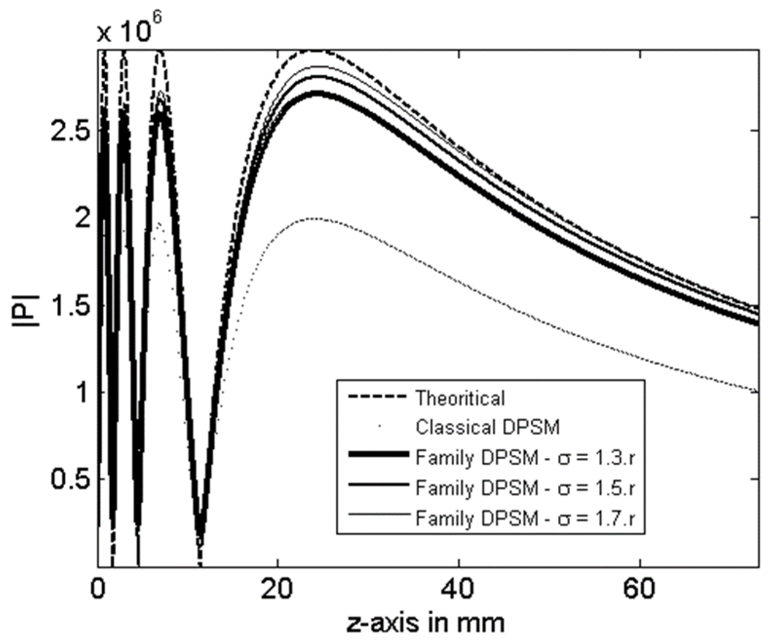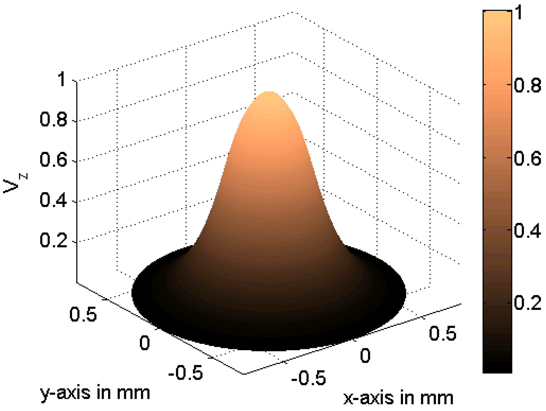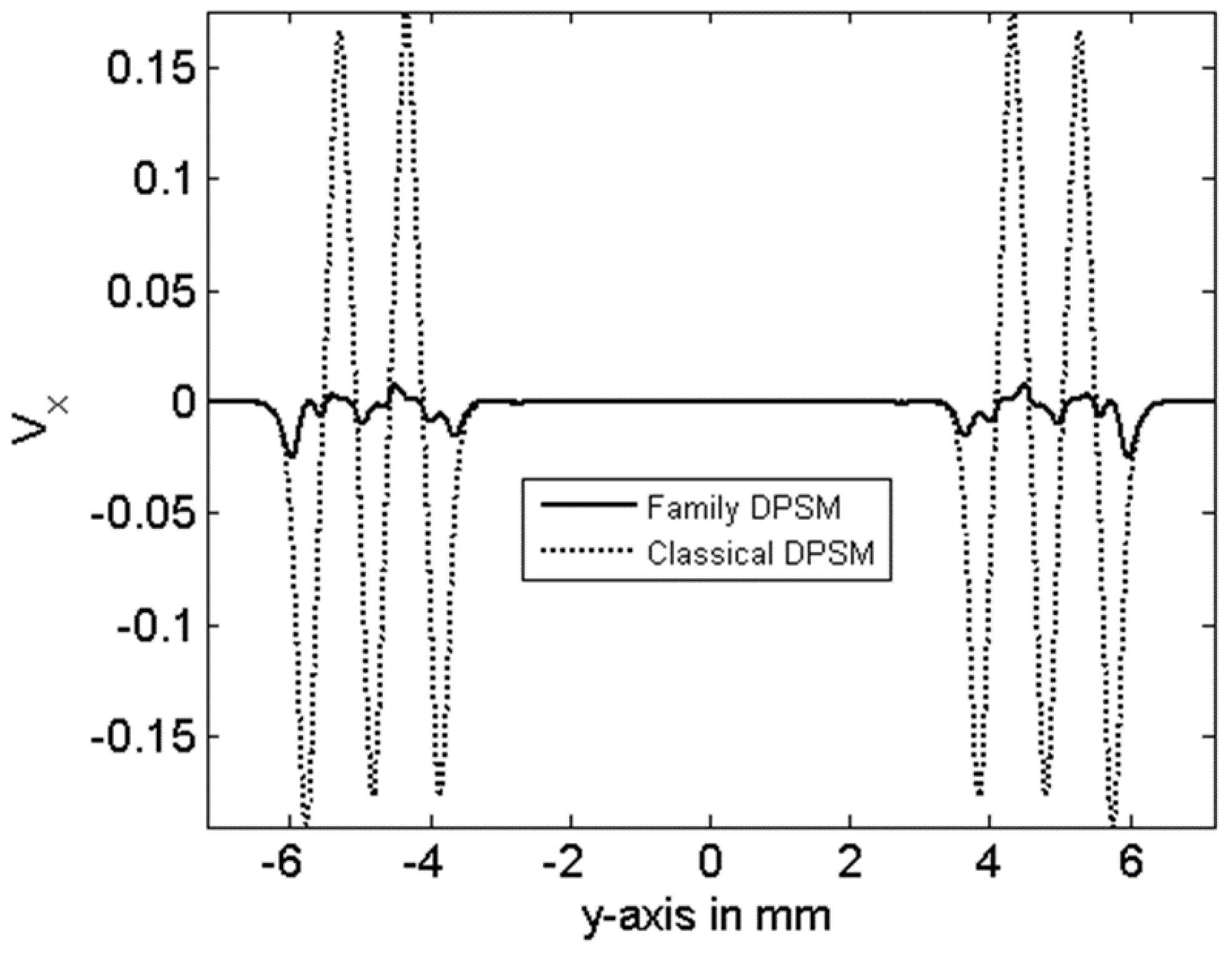However, if such near field solutions are not needed, then the classical DPSM solution with a scaling factor generates accurate results.

4. Conclusions

A new formulation is presented to improve the accuracy of DPSM for the near field computation. The classical DPSM technique works very well for the far field computation but cannot accurately model the near field—the field on the transducer surface and very close to the transducer surface—because DPSM based on the Huygens-Fresnel principle assumes that the point of observation is not very close to the transducer face modeled by distributed point sources. The new formulation explores a new possibility of equivalent source density and makes the DPSM technique accurate in both the near field and the far field. This is achieved by replacing every point source in the classical DPSM formulation by families of quantum sources. An individual family of sources can generate any radiation pattern, unlike an individual point source for which the radiation wave front can only be spherical in an isotropic medium. The new formulation is developed in such a manner that it does not increase the dimension of the square matrix that needs to be inverted for the source strength calculation. Thus, the main advantage of DPSM, that it requires low computational time compared to FEM, is not compromised. In both FEM and classical DPSM formulations the standard approach for improving accuracy is to increase the mesh size for FEM or the number of point sources for DPSM. Both of these approaches significantly increase the computational time and is avoided here. Numerical examples are presented demonstrating the improvement in the computational accuracy with the new technique.

References

- Rayleigh, L. Theory of Sound; Dover Publications: New York, NY, USA, 1965; Volume 2, pp. 162–169. [Google Scholar]
- Morse, P.M.; Ingard, U.K. Theoretical Acoustics; McGraw-Hill: New York, NY, USA, 1968. [Google Scholar]
- Schmerr, L.W. Fundamental of Ultrasonic Nondestructive Evaluation—A Modeling Approach; Plenum Press: New York, NY, USA, 1998. [Google Scholar]
- Kundu, T. (Ed.) Ultrasonic Nondestructive Evaluation: Engineering and Biological Material Characterization; CRC Press: Boca Raton, FL, USA, 2004.
- Harris, G.R. Review of transient field theory for a baffled planar piston. J. Acoust. Soc. Am. 1981, 70, 10–20. [Google Scholar] [CrossRef]
- Sha, K.; Yang, J.; Gan, W.S. A complex virtual source approach for calculating the diffraction beam field generated by a rectangular planar source. IEEE Trans. Ultrason. Ferroelectr. Freq. Control 2003, 50, 890–895. [Google Scholar] [PubMed]
- Stepanishen, P.R. Transient radiation from piston in an infinite planar baffle. J. Acoust. Soc. Am. 1971, 49, 1627–1638. [Google Scholar] [CrossRef]
- Jensen, J.A.; Svendsen, N.B. Calculation of pressure fields from arbitrary shaped, apodized, and excited ultrasound transducers. IEEE Trans. Ultrason. Ferroelectr. Freq. Control 1992, 39, 262–267. [Google Scholar] [CrossRef] [PubMed]
- Ingenito, F.; Cook, B.D. Theoretical investigation of the integrated optical effort produced by sound field radiated from plane piston transducers. J. Acoust. Soc. Am. 1969, 45, 572–577. [Google Scholar] [CrossRef]
- Lockwood, J.C.; Willette, J.G. High-speed method for computing the exact solution for the pressure variations in the near field of a baffled piston. J. Acoust. Soc. Am. 1973, 53, 735–741. [Google Scholar] [CrossRef]
- Scarano, G.; Denisenko, N.; Matteucci, M.; Pappalardo, M. A new approach to the derivation of the impulse response of a rectangular piston. J. Acoust. Soc. Am. 1985, 78, 1109–1113. [Google Scholar] [CrossRef]
- Hah, Z.G.; Sung, K.M. Effect of spatial sampling in the calculation of ultrasonic fields generated by piston transducers. J. Acoust. Soc. Am. 1992, 92, 3403–3408. [Google Scholar] [CrossRef]
- Wu, P.; Kazys, R.; Stepinski, T. Analysis of the numerically implemented angular spectrum approach based on the evaluation of two-dimensional acoustic fields. Part I. Errors due to the discrete Fourier transform and discretization. J. Acoust. Soc. Am. 1995, 99, 1139–1148. [Google Scholar] [CrossRef]
- Lerch, T.P.; Schmerr, L.W.; Sedov, A. Ultrasonic beam models: An edge element approach. J. Acoust. Soc. Am. 1998, 104, 1256–1265. [Google Scholar] [CrossRef]
- Azar, L.; Shi, Y.; Wooh, S.C. Beam focusing behavior of linear phased arrays. NDT E Int. 2000, 33, 189–198. [Google Scholar] [CrossRef]
- Buiochi, F.; Martinez, O.; Ullate, L.G.; Espinosa, F.M. 3D computational method to study the focal laws of transducer arrays for NDE applications. Ultrasonics 2004, 42, 871–876. [Google Scholar] [CrossRef] [PubMed]
- Song, S.J.; Kim, C.H. Simulation of 3-D radiation beam patterns propagated through a planar interface from ultrasonic phased array transducers. Ultrasonics 2002, 40, 519–524. [Google Scholar] [CrossRef]
- Ahmad, R.; Kundu, T.; Placko, D. Modeling of phased array transducers. J. Acoust. Soc. Am. 2005, 117, 1762–1776. [Google Scholar] [CrossRef] [PubMed]
- Park, J.S.; Song, S.J.; Kim, H.J. Calculation of radiation beam field from phased array ultrasonic transducers using expanded Multi-Gaussian beam model. In Advances in Safety and Structural Integrity 2005; Book Series: Solid State Phenomena; Trans Tech Publications: Zürich, Switzerland, 2006; Volume 110, pp. 163–168. [Google Scholar]
- Zhao, X.; Gang, T. A study on non paraxial beam model and ultrasonic measurement model of phased arrays. Ultrasonics 2008, 49, 126–130. [Google Scholar] [CrossRef] [PubMed]
- Placko, D.; Liebeaux, N. Modèle à sources Réparties: Un concept pour le calcul du champ émis par les circuits magnétiques ouverts. In Acte du Deuxième Colloque Interdisciplinaire en Instrumentation (C2I); Hermes: Paris, France, 2001; pp. 523–530. [Google Scholar]
- Placko, D.; Kundu, T. Modeling of ultrasonic field by distributed point source method. In Ultrasonic Nondestructive Evaluation: Engineering and Biological Material Characterization; Kundu, T., Ed.; CRC Press: Boca Raton, FL, USA, 2004; pp. 143–202. [Google Scholar]
- Kundu, T.; Placko, D.; Rahani, E.K.; Yanagita, T.; Dao, C.M. Ultrasonic field modeling: A comparison between analytical, semi-analytical and numerical techniques. IEEE Trans. Ultrason. Ferroelectr. Freq. Control 2010, 57, 2795–2807. [Google Scholar] [CrossRef] [PubMed]
- Wada, Y.; Kundu, T.; Nakamura, K. Mesh-free distributed point source method for modeling viscous fluid layer motion between disks vibrating at ultrasonic frequency. J. Acoust. Soc. Am. 2014, 136, 466–474. [Google Scholar] [CrossRef] [PubMed]
- Placko, D.; Rivollet, A.; Bore, T. Procédé et Dispositif de Modélisation D’une Grandeur Physique d’un Écoulement Fluide (Process and set-up for Modeling a Physical Value in a Fuid Flow). French Patent Appl. 1454675, 23 May 2014. [Google Scholar]
- Jarvis, A.J.C.; Cegla, F.B. Scattering of near normal incidence SH waves by sinusoidal and rough surfaces in 3-D: Comparison to the scalar wave approximation. IEEE Trans. Ultrason. Ferroelectr. Freq. Control 2014, 61, 1179–1190. [Google Scholar] [CrossRef] [PubMed]
- Bore, T.; Placko, D.; Taillade, F.; Sabouroux, P. Electromagnetic characterization of grouting materials of bridge post tensioned ducts for NDT using capacitive probe. NDT E Int. 2013, 60, 110–120. [Google Scholar] [CrossRef]
- Rahani, E.K.; Kundu, T. Gaussian DPSM (G-DPSM) and Element Source Method (ESM) modifications to DPSM for ultrasonic field modeling. Ultrasonics 2011, 51, 625–631. [Google Scholar] [CrossRef] [PubMed]
- Placko, D.; Bore, T.; Kundu, T. Distributed point source method for modeling and imaging in electrostatic and electromagnetic problems. In Ultrasonic and Electromagnetic NDE for Structure and Material Characterization: Engineering and Biomedical Applications; Kundu, T., Ed.; CRC Press: Boca Raton, FL, USA, 2004; pp. 249–294. [Google Scholar]
© 2016 by the authors; licensee MDPI, Basel, Switzerland. This article is an open access article distributed under the terms and conditions of the Creative Commons Attribution (CC-BY) license (http://creativecommons.org/licenses/by/4.0/).
Share and Cite
Placko, D.; Bore, T.; Kundu, T. Family of Quantum Sources for Improving Near Field Accuracy in Transducer Modeling by the Distributed Point Source Method. Appl. Sci. 2016, 6, 302. https://doi.org/10.3390/app6100302
Placko D, Bore T, Kundu T. Family of Quantum Sources for Improving Near Field Accuracy in Transducer Modeling by the Distributed Point Source Method. Applied Sciences. 2016; 6(10):302. https://doi.org/10.3390/app6100302
Chicago/Turabian StylePlacko, Dominique, Thierry Bore, and Tribikram Kundu. 2016. "Family of Quantum Sources for Improving Near Field Accuracy in Transducer Modeling by the Distributed Point Source Method" Applied Sciences 6, no. 10: 302. https://doi.org/10.3390/app6100302
APA StylePlacko, D., Bore, T., & Kundu, T. (2016). Family of Quantum Sources for Improving Near Field Accuracy in Transducer Modeling by the Distributed Point Source Method. Applied Sciences, 6(10), 302. https://doi.org/10.3390/app6100302