Round-Off Noise of Multiplicative FIR Filters Implemented on an FPGA Platform

Abstract
:1. Introduction


 (Here ωn is the normalized angular frequency: ωn = ωTS, and TS is the sampling period.) can also be realized using the following procedure [1,4].
- Design an IIR filter that approximates
![Applsci 04 00099 i069]() .
. - Approximate the poles of the IIR filter with the MFIR structure.
- Cascade to every zero in the resulting MFIR filter its reciprocal with respect to the unit circle.

 and approximating the real pole λ' of Hr'(z) with:

 and approximating the poles λ' = r'e+jθ' and λ'* = r'e−jθ' of Hc'(z) with:

2. The Round-Off Noise Model
2.1. Introduction
2.2. The Round-Off Noise Model
- every sample of the noise source is uncorrelated with the previous sample,
- all noise sources are uncorrelated,
- the noise sources are uncorrelated with the input signal,
- every noise source is a time discrete stationary zero mean white random process with output variance q2/12. Here, q is the smallest quantization step (q = 2−b where b is the number of bits (without the sign bit) used to quantize the signal).
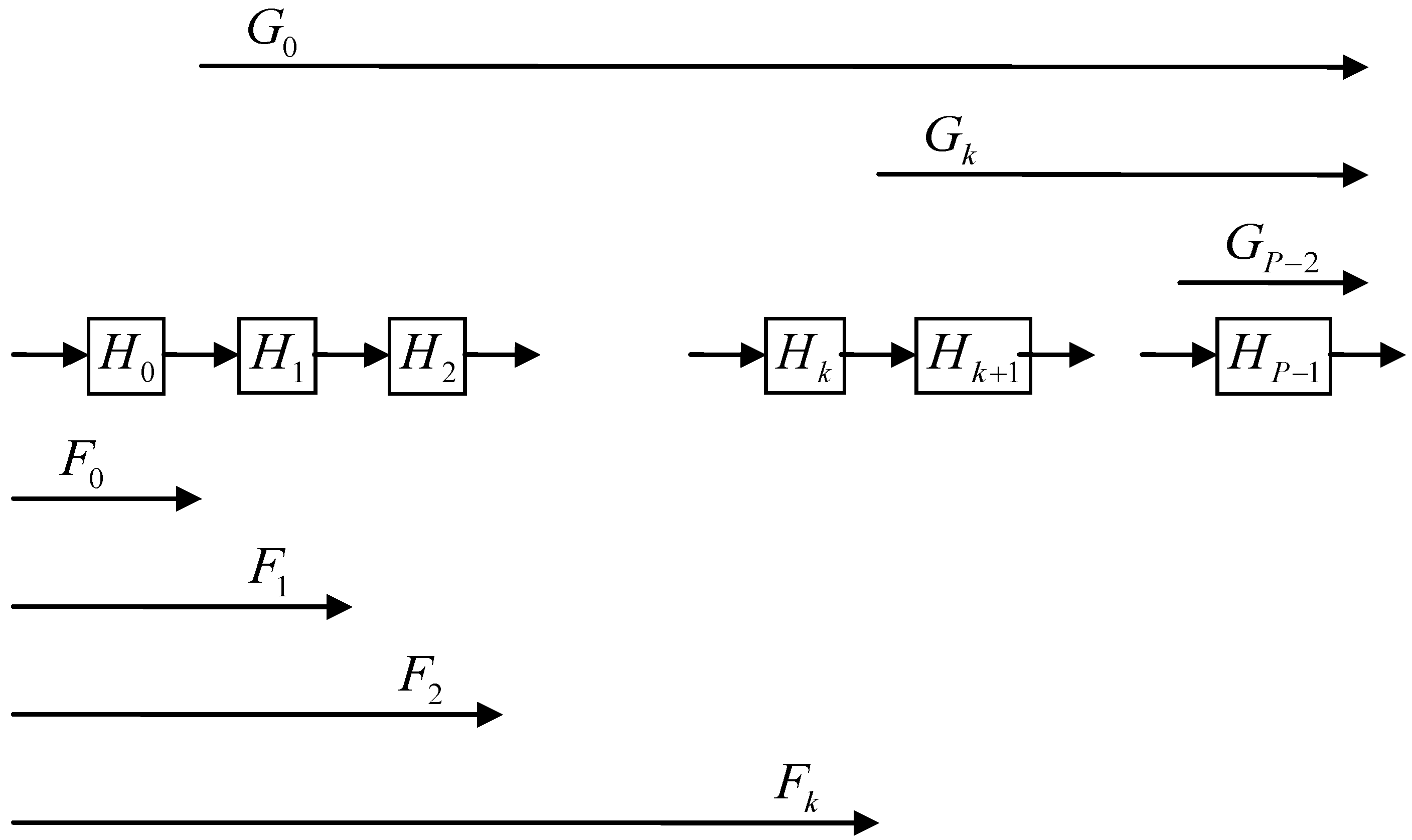
2.3. Symbol Conventions and Transfer Functions
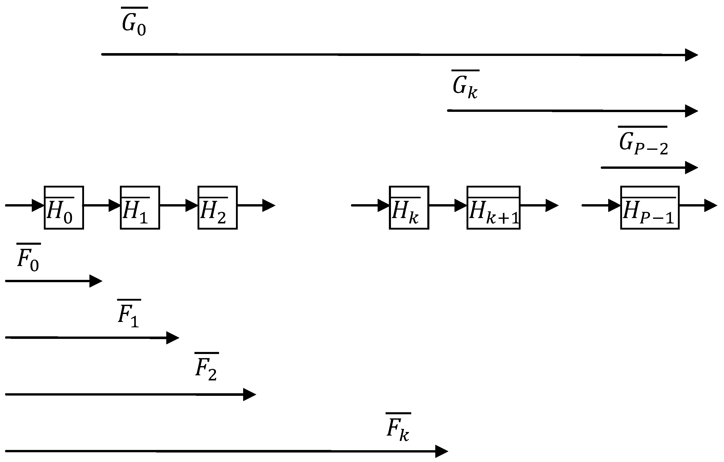
 or in short form Hk. The total filter transfer function is written as H(z), or
  . A (general) stage with rounding and scaling is indicated by Hk (z),
  or in short form Hk. The respective scaling factors per stage are indicated by Sk. The time samples of the round-off noise source are indicated by ek(n) (where n is the discrete time index) or in short form ek. The noise variance of a noise source is given by
  .
.


3. The General Scaling Methods
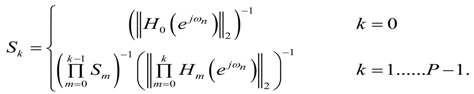
- For L2 bound scaling, the scaling factors are determined by:where
![Applsci 04 00099 i010]()
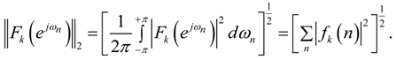
![Applsci 04 00099 i091]() is defined as the L2 norm in the frequency domain, given by:
Here, fk(n) are the impulse response samples of the filter given by the transfer function Fk (z). The recursive version of Equation (10) can be used to calculate the scale factor per stage. It is given by:
is defined as the L2 norm in the frequency domain, given by:
Here, fk(n) are the impulse response samples of the filter given by the transfer function Fk (z). The recursive version of Equation (10) can be used to calculate the scale factor per stage. It is given by:![Applsci 04 00099 i011]() The following holds when L2 bound scaling is used: if the RMS value (over ωn) of the input signal is bounded by unity, the RMS value (over ωn) of the signal at each stage output will be bounded by unity.
The following holds when L2 bound scaling is used: if the RMS value (over ωn) of the input signal is bounded by unity, the RMS value (over ωn) of the signal at each stage output will be bounded by unity.![Applsci 04 00099 i012]()
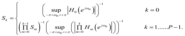
- For infinity bound scaling, L∞, the scaling factors are determined by:The recursive version of Equation (13) can be used to calculate the scale factor per stage. It is given by:
![Applsci 04 00099 i013]() The L∞ bound scaling sets the maximum of the frequency responses of all respective Fk(ejωn) at 0 dB.
The L∞ bound scaling sets the maximum of the frequency responses of all respective Fk(ejωn) at 0 dB.![Applsci 04 00099 i014]()
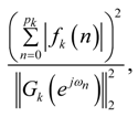
- For absolute bound scaling, the scaling factors are determined by:where fk(n) are the impulse response samples of the filter given by the transfer function Fk(z). pk is the length of the impulse response. Equation (15) in recursive form yields:
![Applsci 04 00099 i015]() Absolute bound scaling is based on the reasoning that if the peak value of the input signal is bounded by unity, the peak absolute value of the signal at each stage output will be bounded by unity when absolute bound scaling is used. The absolute bound scaling criterion is avoiding overflow in all cases.
Absolute bound scaling is based on the reasoning that if the peak value of the input signal is bounded by unity, the peak absolute value of the signal at each stage output will be bounded by unity when absolute bound scaling is used. The absolute bound scaling criterion is avoiding overflow in all cases.![Applsci 04 00099 i016]()


4. The Ordering of the Stages
4.1. The Round-Off Output Noise Variance
. The input signal of the filter has an amplitude in the interval (−1, +1). In case b + 1 bits (b bits + a sign bit) are used to represent the signal in two’s complement, the variance of the noise generated by one round-off noise source is (under the assumptions of Section 2.2) given by:


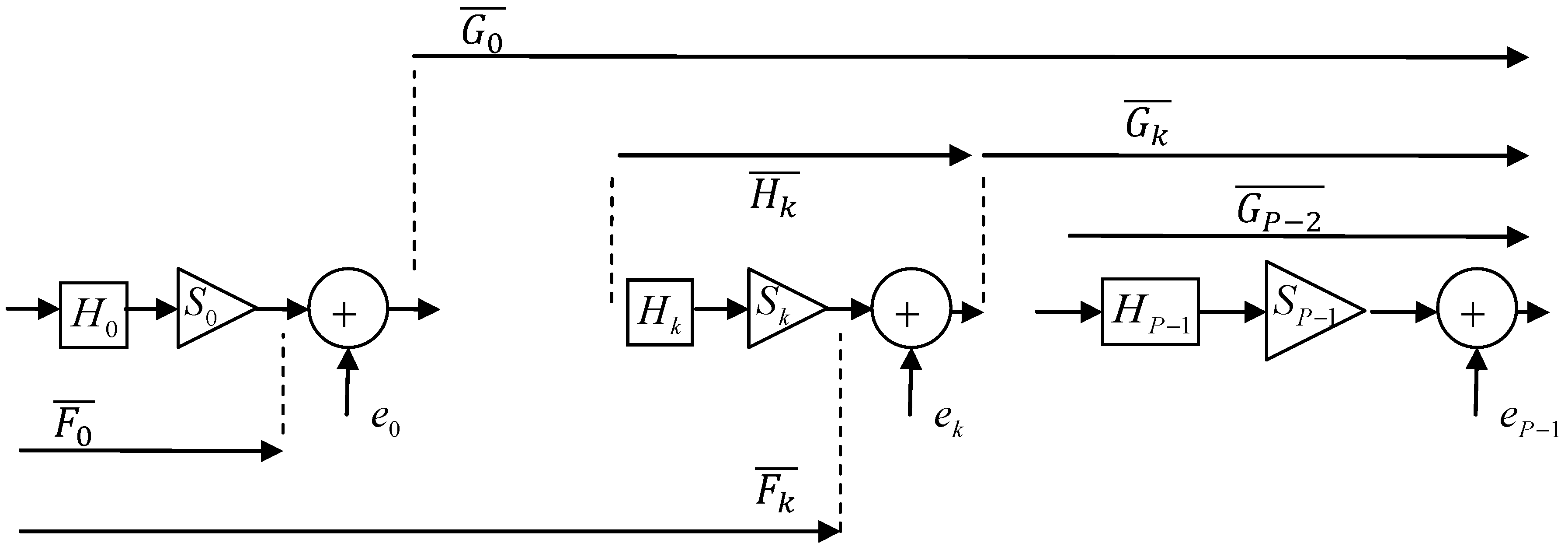
 (for any k) as small as possible. This approach minimizes the output round-off noise variance. However, in Equation (23), the transfer function from a noise source k to the output is scaled, implying that the optimal ordering must be derived from the scaled stage equations, which is rather inconvenient. Therefore, Equation (23) will be further worked out. It is clear from Figure 3 and Equation (7) that Equation (22) can be written as:


 is minimal, i.e., an optimal ordering must be found to minimize this sum.
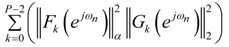
- In case of L2 bound scaling (α = 2),
![Applsci 04 00099 i075]() and
and ![Applsci 04 00099 i076]() in every sum term will have the same contribution, implying that the ordering of the stages has no importance. (I.e., in case of ordering from i = 0 to i = P − 1 and using L2 bound scaling, Equation (27) yields:
in every sum term will have the same contribution, implying that the ordering of the stages has no importance. (I.e., in case of ordering from i = 0 to i = P − 1 and using L2 bound scaling, Equation (27) yields: ![Applsci 04 00099 i077]() . In case of ordering from i = P − 1 to i = 0 and using L2 bound scaling, Equation (27) yields:
. In case of ordering from i = P − 1 to i = 0 and using L2 bound scaling, Equation (27) yields: ![Applsci 04 00099 i078]() . Two identical equations are obtained.)
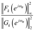
. Two identical equations are obtained.) - If infinity bound scaling, L∞, is considered (α = ∞), the optimal ordering will be determined by the ratio:
![Applsci 04 00099 i028]() for every k ϵ {0,1, …, P − 2}. In case this ratio is significantly larger than 1 for every k value, it is best to order the stages from small peak gain to large peak gain. In case this ratio is not significantly larger than 1, the optimal ordering should be determined exhaustively.
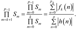
for every k ϵ {0,1, …, P − 2}. In case this ratio is significantly larger than 1 for every k value, it is best to order the stages from small peak gain to large peak gain. In case this ratio is not significantly larger than 1, the optimal ordering should be determined exhaustively. - In case of absolute bound scaling the equivalent of Equation (25) is given by:Here h(n) are the impulse response (having a length p) samples of the filter given by the transfer function H(z). Applying Equation (29) on Equation (22) and using Equation (7) yields:
![Applsci 04 00099 i029]() and by applying Equation (11):
and by applying Equation (11):![Applsci 04 00099 i030]() As for infinity bound scaling, the optimal ordering to obtain a minimal output round-off noise variance is determined by the ratio:
As for infinity bound scaling, the optimal ordering to obtain a minimal output round-off noise variance is determined by the ratio:![Applsci 04 00099 i031]() for every k ϵ {0,1, …, P − 2}.
for every k ϵ {0,1, …, P − 2}.![Applsci 04 00099 i032]() In case this ratio is significantly larger than 1 for every k value, it is best to order the stages in increasing coefficient magnitude, i.e., the stage with the largest coefficient(s) at the end. In case the ratio is not significantly larger than 1, the optimal ordering should be determined exhaustively.
In case this ratio is significantly larger than 1 for every k value, it is best to order the stages in increasing coefficient magnitude, i.e., the stage with the largest coefficient(s) at the end. In case the ratio is not significantly larger than 1, the optimal ordering should be determined exhaustively.


4.2. The Signal to Round-off Noise Ratio
 . The variance of the discrete output signal y(n) of the filter will be indicated by
  . All calculations presented in this section are based on the conditions that the input signal x(n) is zero mean and has a constant, frequency independent, Probability Density Function (PDF). , the output signal variance of the filter is given by:


 is the sum of the squared impulse response samples of the (scaled and rounded) filter.
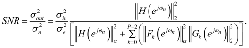
- In case of L2 or L∞ bound scaling, Equation (34) can be written as (using Equation (10) or Equation (13) as appropriate):where α = 2 or α = ∞, respectively. Combining Equations (36) and (27) yields.
![Applsci 04 00099 i036]()
![Applsci 04 00099 i037]()
- In case of absolute bound scaling, the SNR is given by:
![Applsci 04 00099 i038]()

 is dependent on the type of rounding used and the number of bits that are used to quantize the signal in the filter structure. depends on the input signal. Quantization and input signal independent factors are given by:


 in Equation (39) is independent of the stage ordering, implying that the stage ordering has no impact on the SNR. For a given ordering of the stages, it is clear from Equations (39–41) and (43) that


5. The SNR of MFIR Filters
5.1. The Transfer Functions
 or Mi.


 ) = M ( ) and GP−1 ( ) = 1 (see Figure 2 and Figure 3).
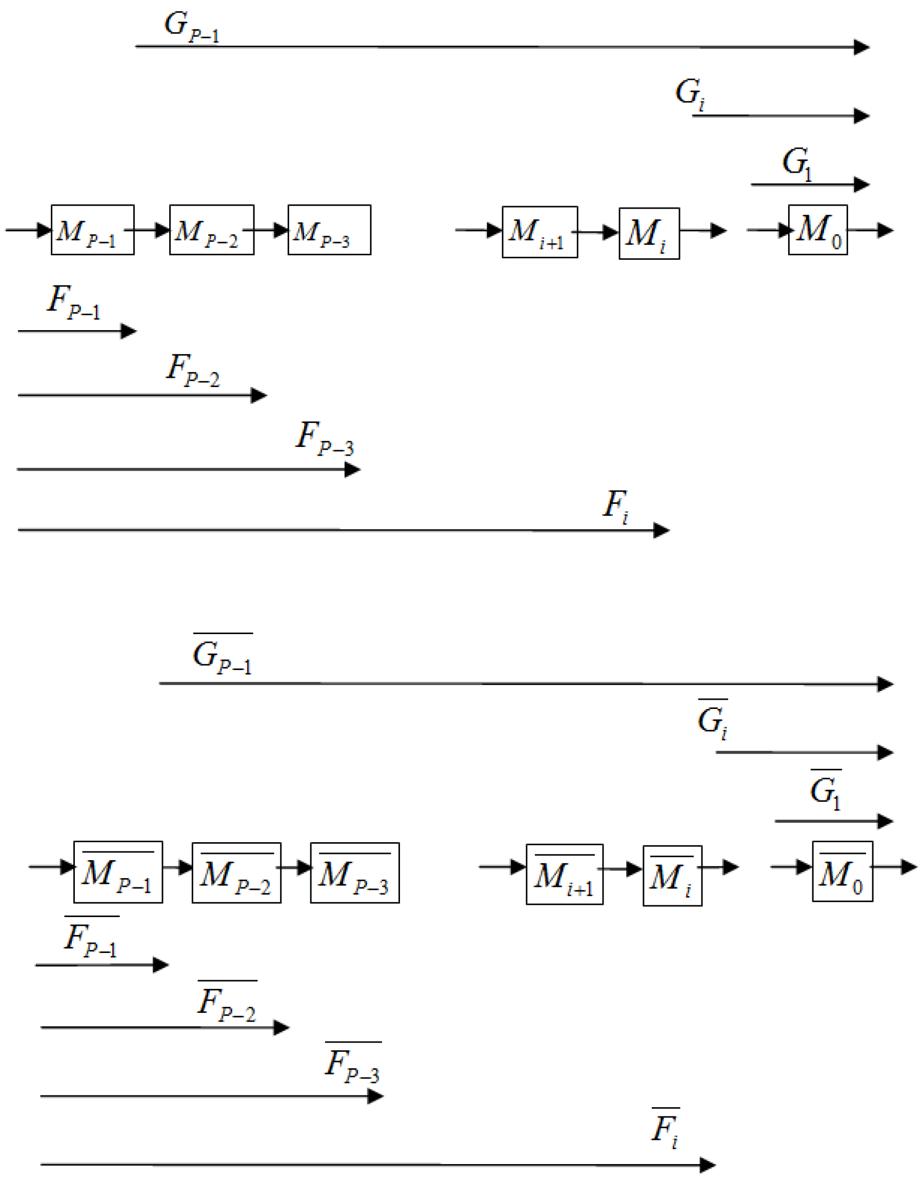


5.2. The Scaling Factors

| Forward ordering | Reverse ordering | |
|---|---|---|
| L2 bound |  |  |
| Infinity bound | 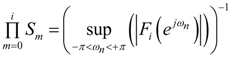 |  |
| Absolute bound |  |  |
| Forward ordering | fi (n) or fi (n) |
| Real pole | 0 → pi = 2i+1 − 1 |
| Real pole linear phase | 0 → pi = 2i+2 − 2 |
| Complex-conjugate pole pair | 0 → pi = 2i+2 − 2 |
| Complex-conjugate pole pair linear phase | 0 → pi = 2i+3 − 4 |
| Reverse ordering | fi (n) or fi (n) |
| Real pole | 0 → pi = 2P − 2i |
| Real pole linear phase | 0 → pi = 2P+1 − 2i+1 |
| Complex-conjugate pole pair | 0 → pi = 2P+1 − 2i+1 |
| Complex-conjugate pole pair linear phase | 0 → pi = 2P+2 − 2i+2 |
5.3. The SNR and Optimal Ordering for MFIR Filters
5.3.1. General MFIR SNR Expressions


 and
and  are given by Equations (47) and (49) respectively. The value of pi is given in Table 2 for forward ordering. m(n) are the impulse response samples of the total MFIR filter. The value p in
  in Equation (57) is the length of the total MFIR filter impulse response and can be found by setting i = P − 1 in Table 2 for forward ordering.

 and are given by Equations (50) and (53) respectively. The value of pi is given in Table 2 for reverse ordering. The value p in in Equation (60) is the length of the total MFIR filter impulse response and can be found by setting i = 0 in Table 2 for reverse ordering.
 | Approximation of | Scaling type | Ordering | Range | Figure |
|---|---|---|---|---|
| Real pole | L2 | Forward and Reverse | |λ| ϵ [0.1, 1) | Figure 6 |
| Real Pole | Abs and Inf. | Forward and Reverse | |λ| ϵ [0.1, 1) | Figure 7 |
| Real Pole Linear Phase | L2 | Forward and Reverse | |λ| ϵ [0.1, 1) | Figure 8 |
| Real Pole Linear Phase | Abs and Inf. | Forward and Reverse | |λ| ϵ [0.1, 1) | Figure 9 |
| Compl. Conj. Pole pair | L2 | Forward and Reverse | r = 0.9 θ ϵ [0, π) | Figure 10 |
| Compl. Conj. Pole pair | Inf | Forward and Reverse | r = 0.9 θ ϵ [0, π) | Figure 11 |
| Compl. Conj. Pole pair | Abs | Forward and Reverse | r = 0.9 θ ϵ [0, π) | Figure 12 |
| Compl. Conj. Pole pair | Inf | Reverse | r = 0.8; 0.85; 0.9; 0.95 θ ϵ [0, π) | Figure 13 |
| Compl. Conj. Pole pair | L2, Inf, Abs | Forward and Reverse | r = 0.9 θ ϵ [0, π) | Figure 14 |
| Compl. Conj. Pole pair, Lin Phase | L2, Inf, Abs | Forward | r = 0.9 θ ϵ [0, π) | Figure 15 |
| Compl. Conj. Pole pair, Lin Phase | L2, Inf, Abs | Reverse | r = 0.9 θ ϵ [0, π) | Figure 16 |
| Compl. Conj. Pole pair, Lin Phase | Inf | Reverse | r = 0.8; 0.85; 0.9; 0.95 θ ϵ [0, π) | Figure 17 |
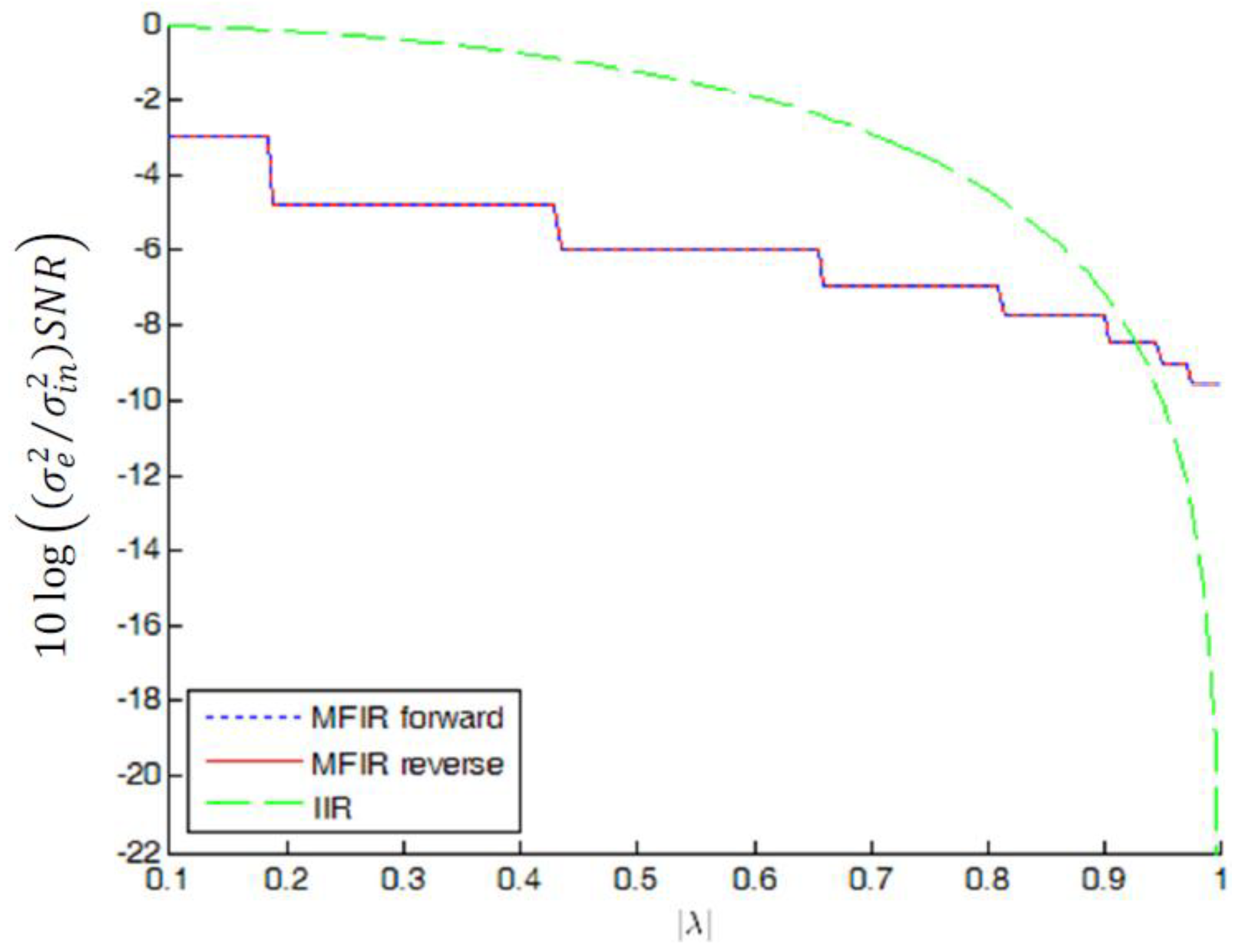
5.3.2. SNR Performance of an MFIR Filter Approximating a Real Pole Filter
 values for real poles |λ| in the interval [0.1, 1). In case of the MFIR approximation, for each |λ| value, the required number of stages, P, is determined to obtain a maximum difference of |0.01| dB between the MFIR magnitude response and the magnitude response of the approximated IIR filter. The edges in the curves indicate where an extra MFIR stage is added to fulfill this requirement. The IIR filter results are based on ([10], Equation 12.148):
 for real poles |λ| in the interval [0.1, 1) in case of L2 bound scaling. (The MFIR forward and MFIR reverse results are superimposed).
for real poles |λ| in the interval [0.1, 1) in case of L2 bound scaling. (The MFIR forward and MFIR reverse results are superimposed).
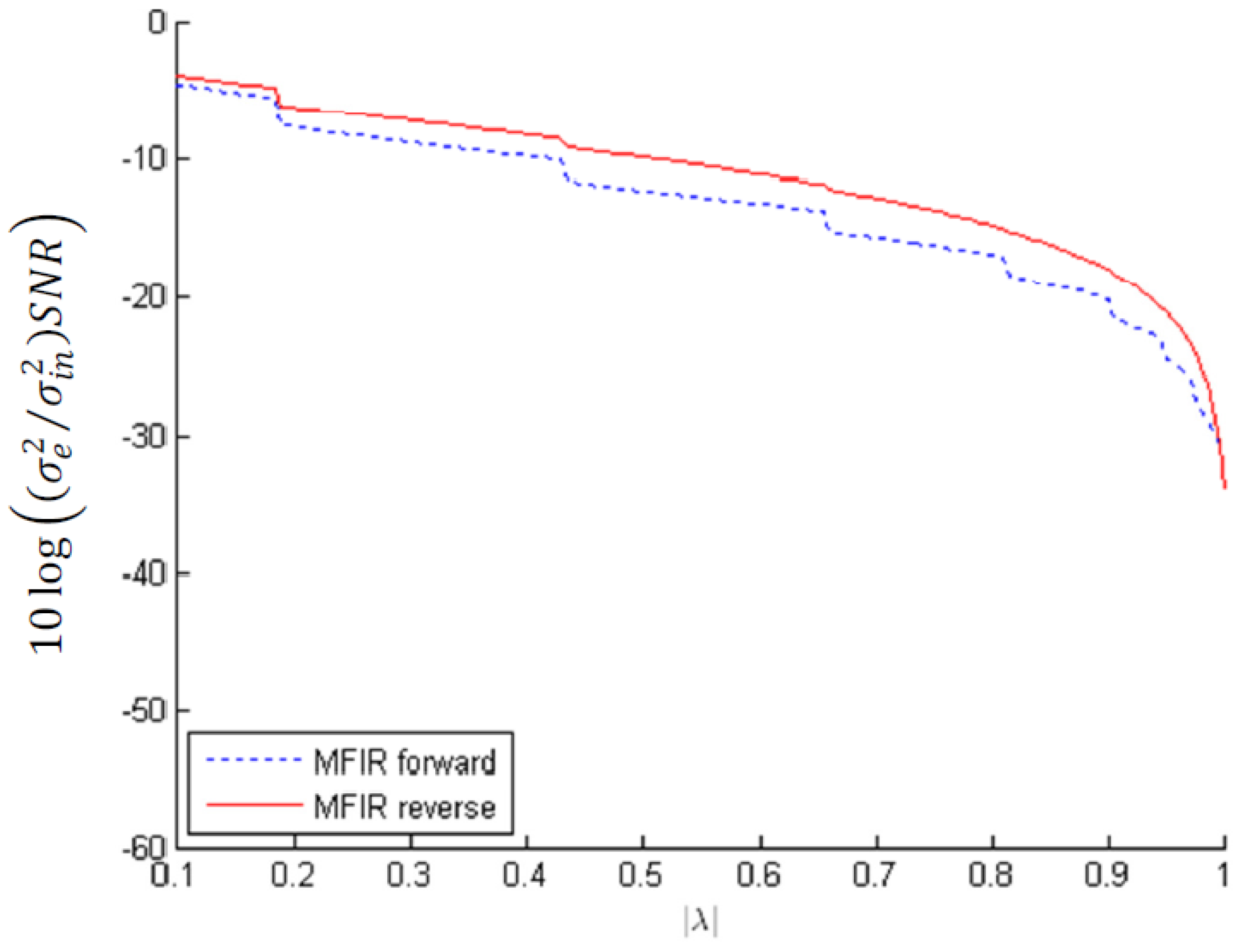
for real poles |λ| in the interval [0.1, 1) in case of L2 bound scaling. (The MFIR forward and MFIR reverse results are superimposed). for real poles |λ| in the interval [0.1, 1) in case of absolute or infinity bound scaling.
for real poles |λ| in the interval [0.1, 1) in case of absolute or infinity bound scaling.
for real poles |λ| in the interval [0.1, 1) in case of absolute or infinity bound scaling.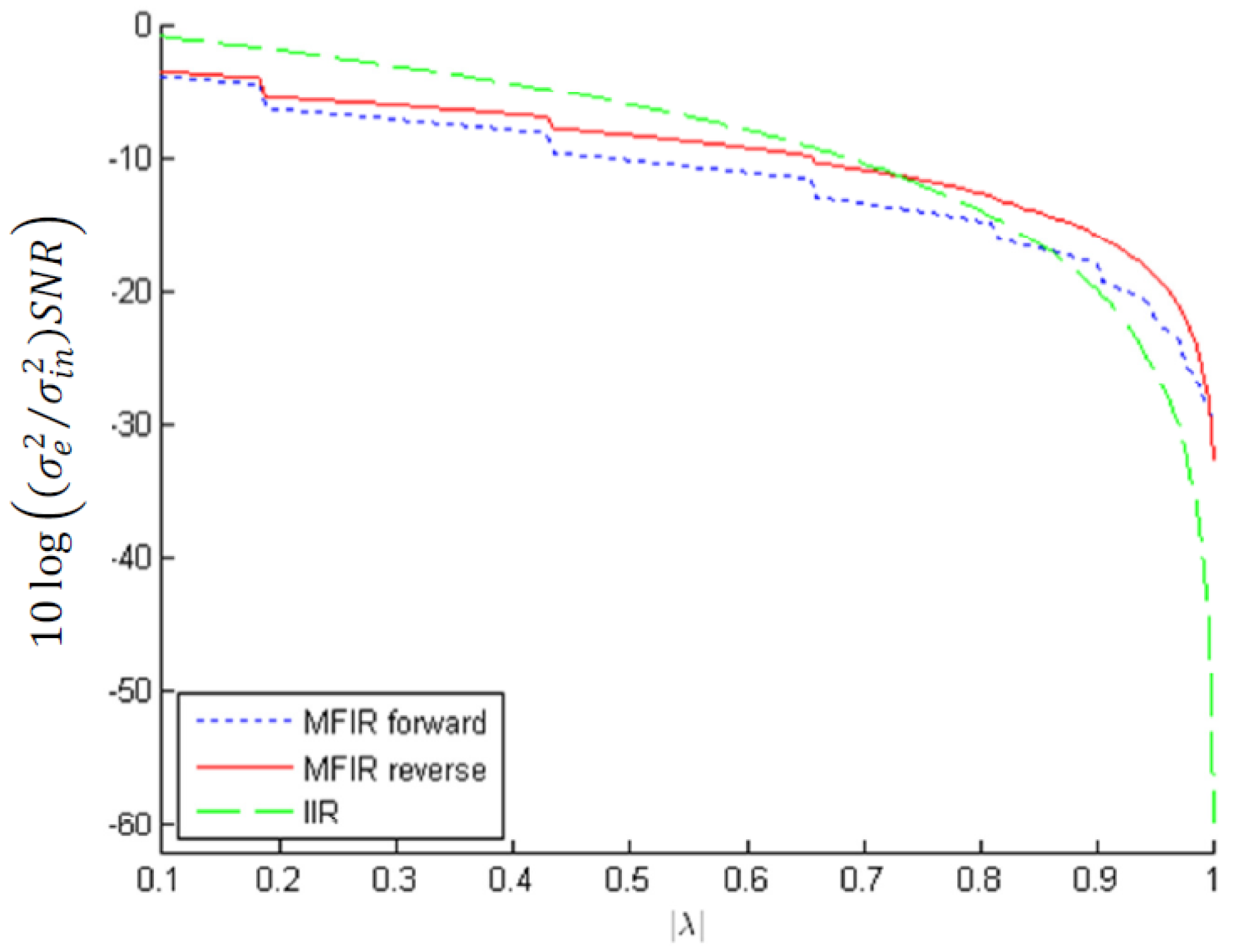 of MFIR filters approximating the squared magnitude response of real poles |λ| in the interval [0.1, 1) in case of L2 bound scaling. (The MFIR forward and MFIR reverse results are superimposed).
of MFIR filters approximating the squared magnitude response of real poles |λ| in the interval [0.1, 1) in case of L2 bound scaling. (The MFIR forward and MFIR reverse results are superimposed).
of MFIR filters approximating the squared magnitude response of real poles |λ| in the interval [0.1, 1) in case of L2 bound scaling. (The MFIR forward and MFIR reverse results are superimposed).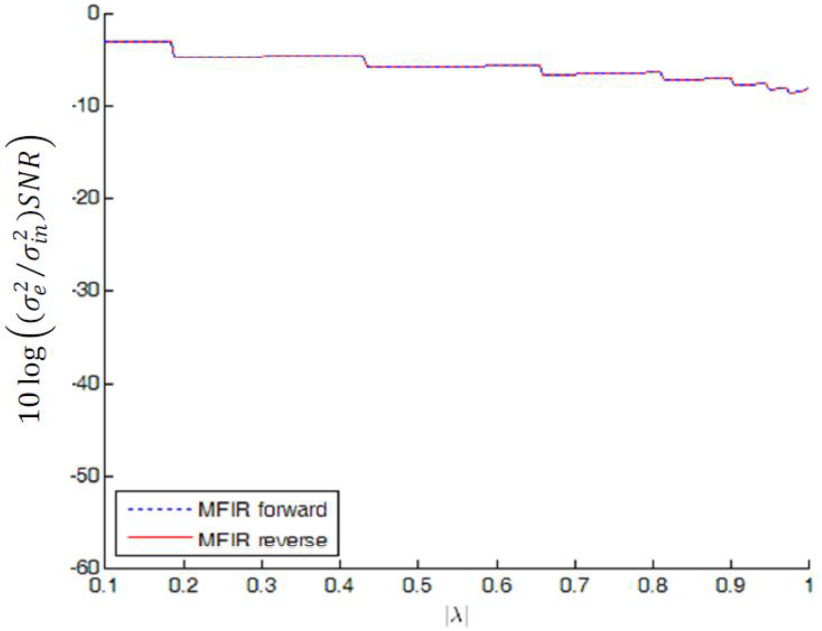 of MFIR filters approximating the squared magnitude response of real poles |λ| in the interval [0.1, 1) in case of absolute and/ or infinity bound scaling.
of MFIR filters approximating the squared magnitude response of real poles |λ| in the interval [0.1, 1) in case of absolute and/ or infinity bound scaling.
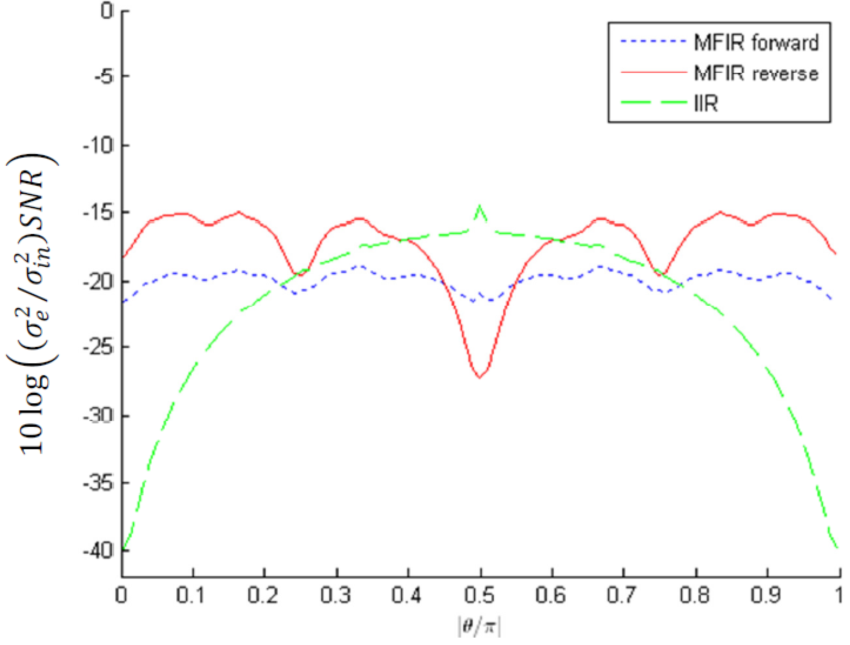
of MFIR filters approximating the squared magnitude response of real poles |λ| in the interval [0.1, 1) in case of absolute and/ or infinity bound scaling. for complex-conjugate pole pairs with magnitude 0.9 and L2 bound scaling; The MFIR approximation uses P = 7 stages. (The MFIR forward and MFIR reverse results are superimposed).
for complex-conjugate pole pairs with magnitude 0.9 and L2 bound scaling; The MFIR approximation uses P = 7 stages. (The MFIR forward and MFIR reverse results are superimposed).
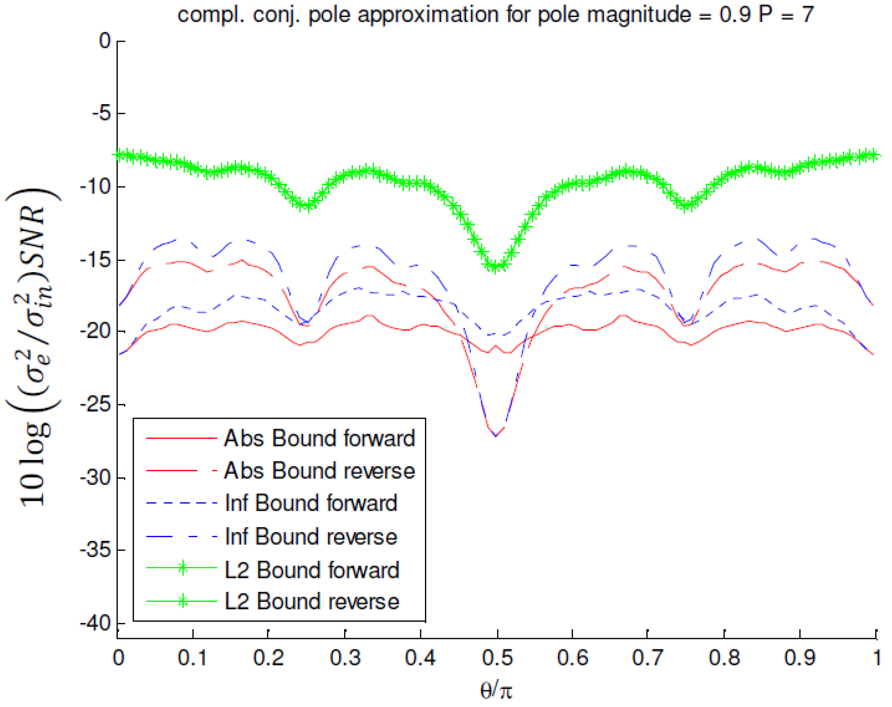
for complex-conjugate pole pairs with magnitude 0.9 and L2 bound scaling; The MFIR approximation uses P = 7 stages. (The MFIR forward and MFIR reverse results are superimposed). for complex-conjugate pole pairs with magnitude 0.9 and infinity bound scaling; The MFIR approximation uses P = 7 stages.
for complex-conjugate pole pairs with magnitude 0.9 and infinity bound scaling; The MFIR approximation uses P = 7 stages.
for complex-conjugate pole pairs with magnitude 0.9 and infinity bound scaling; The MFIR approximation uses P = 7 stages. 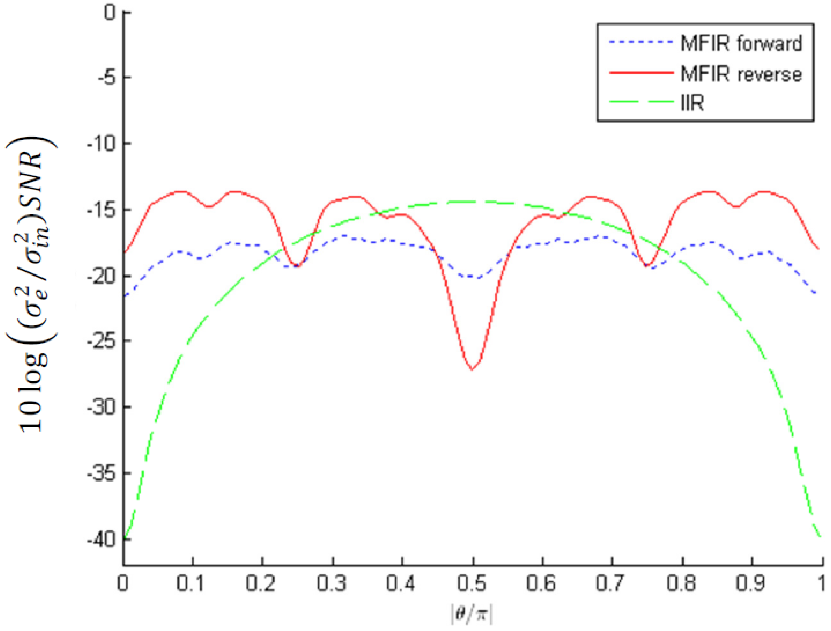 for complex-conjugate pole pairs with magnitude 0.9 and absolute bound scaling; The MFIR approximation uses P = 7 stages.
for complex-conjugate pole pairs with magnitude 0.9 and absolute bound scaling; The MFIR approximation uses P = 7 stages.
for complex-conjugate pole pairs with magnitude 0.9 and absolute bound scaling; The MFIR approximation uses P = 7 stages. in function of pole magnitude r and pole angle θ, in case of infinity bound scaling and reverse ordering. (surface = MFIR; discrete curves = IIR filter).
in function of pole magnitude r and pole angle θ, in case of infinity bound scaling and reverse ordering. (surface = MFIR; discrete curves = IIR filter).
in function of pole magnitude r and pole angle θ, in case of infinity bound scaling and reverse ordering. (surface = MFIR; discrete curves = IIR filter).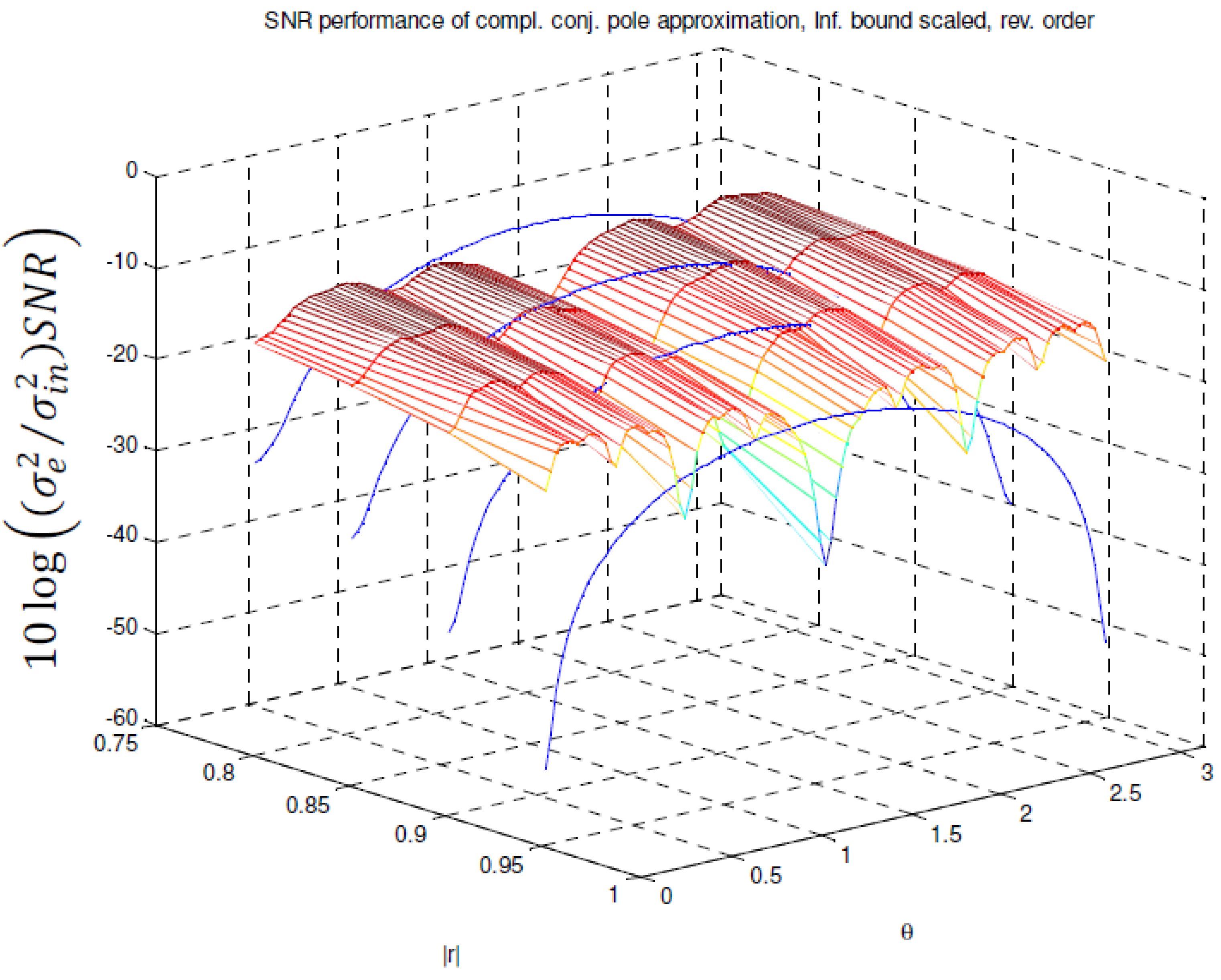 of an MFIR filter approximating a complex-conjugate pole pair with magnitude 0.9, and P = 7.
of an MFIR filter approximating a complex-conjugate pole pair with magnitude 0.9, and P = 7.
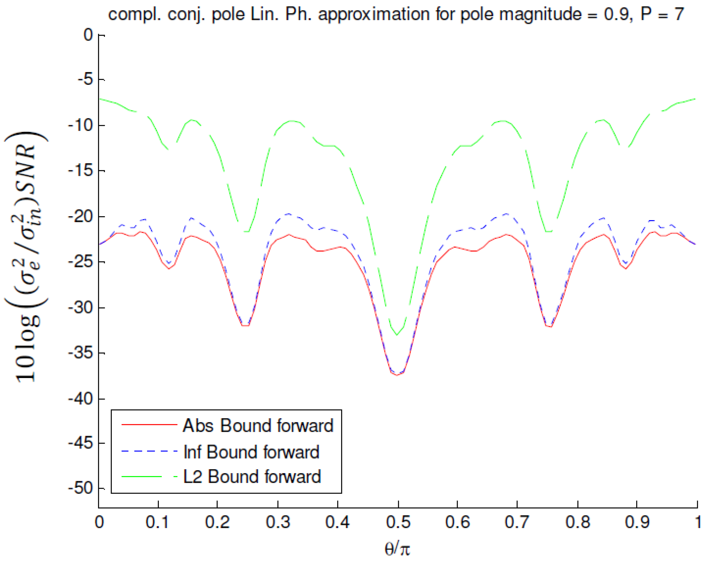
of an MFIR filter approximating a complex-conjugate pole pair with magnitude 0.9, and P = 7. of a linear phase MFIR filter approximating the squared magnitude response of a complex-conjugate pole pair with magnitude 0.9 and P = 7 in forward ordering.
of a linear phase MFIR filter approximating the squared magnitude response of a complex-conjugate pole pair with magnitude 0.9 and P = 7 in forward ordering.
of a linear phase MFIR filter approximating the squared magnitude response of a complex-conjugate pole pair with magnitude 0.9 and P = 7 in forward ordering. of a linear phase MFIR filter approximating the squared magnitude response of a complex-conjugate pole pair with magnitude 0.9 and P = 7 in reverse ordering.
of a linear phase MFIR filter approximating the squared magnitude response of a complex-conjugate pole pair with magnitude 0.9 and P = 7 in reverse ordering.
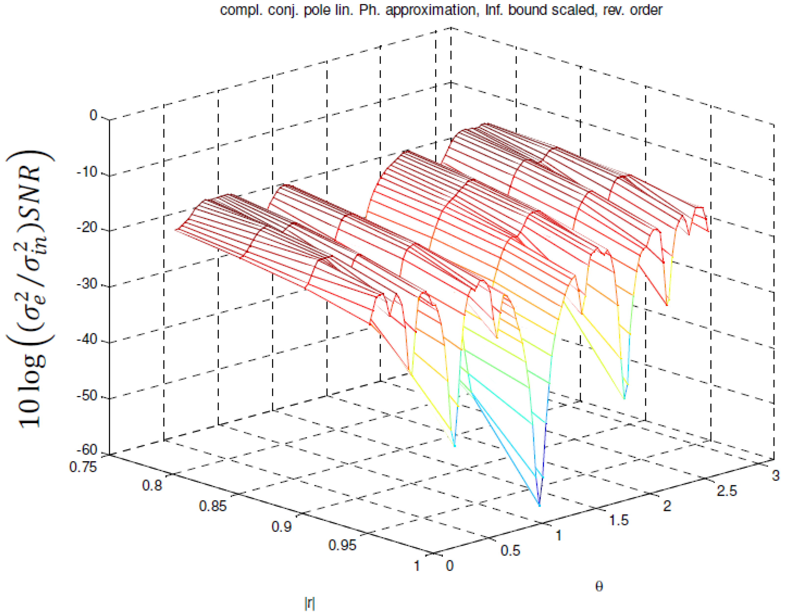
of a linear phase MFIR filter approximating the squared magnitude response of a complex-conjugate pole pair with magnitude 0.9 and P = 7 in reverse ordering.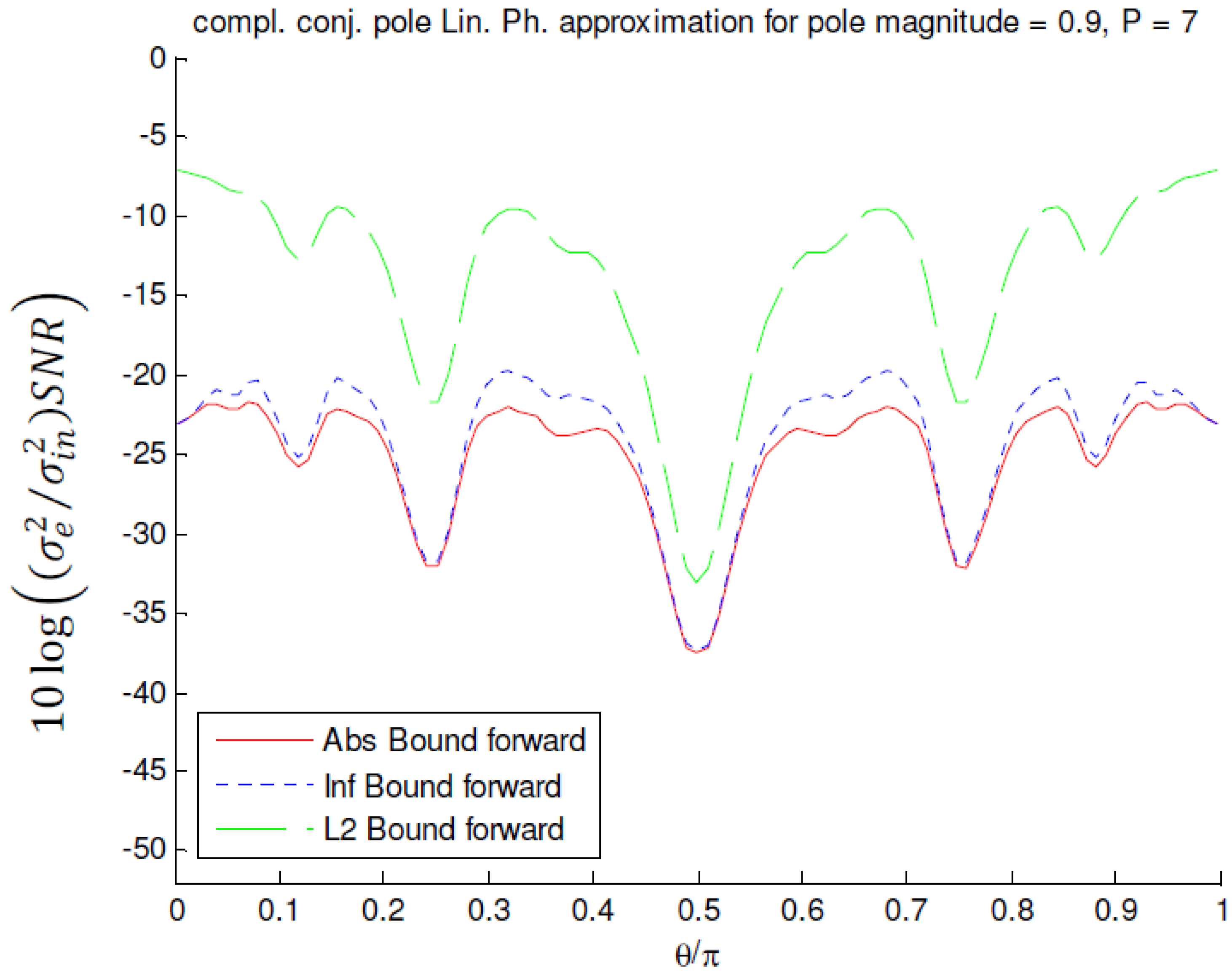 of a linear phase MFIR filter in function of the pole angle and magnitude in case of infinity bound scaling and reverse ordering.
of a linear phase MFIR filter in function of the pole angle and magnitude in case of infinity bound scaling and reverse ordering.
of a linear phase MFIR filter in function of the pole angle and magnitude in case of infinity bound scaling and reverse ordering.
5.3.3. SNR Performance of a Linear Phase MFIR Filter Approximating the Squared Magnitude Response of a Real Pole Filter
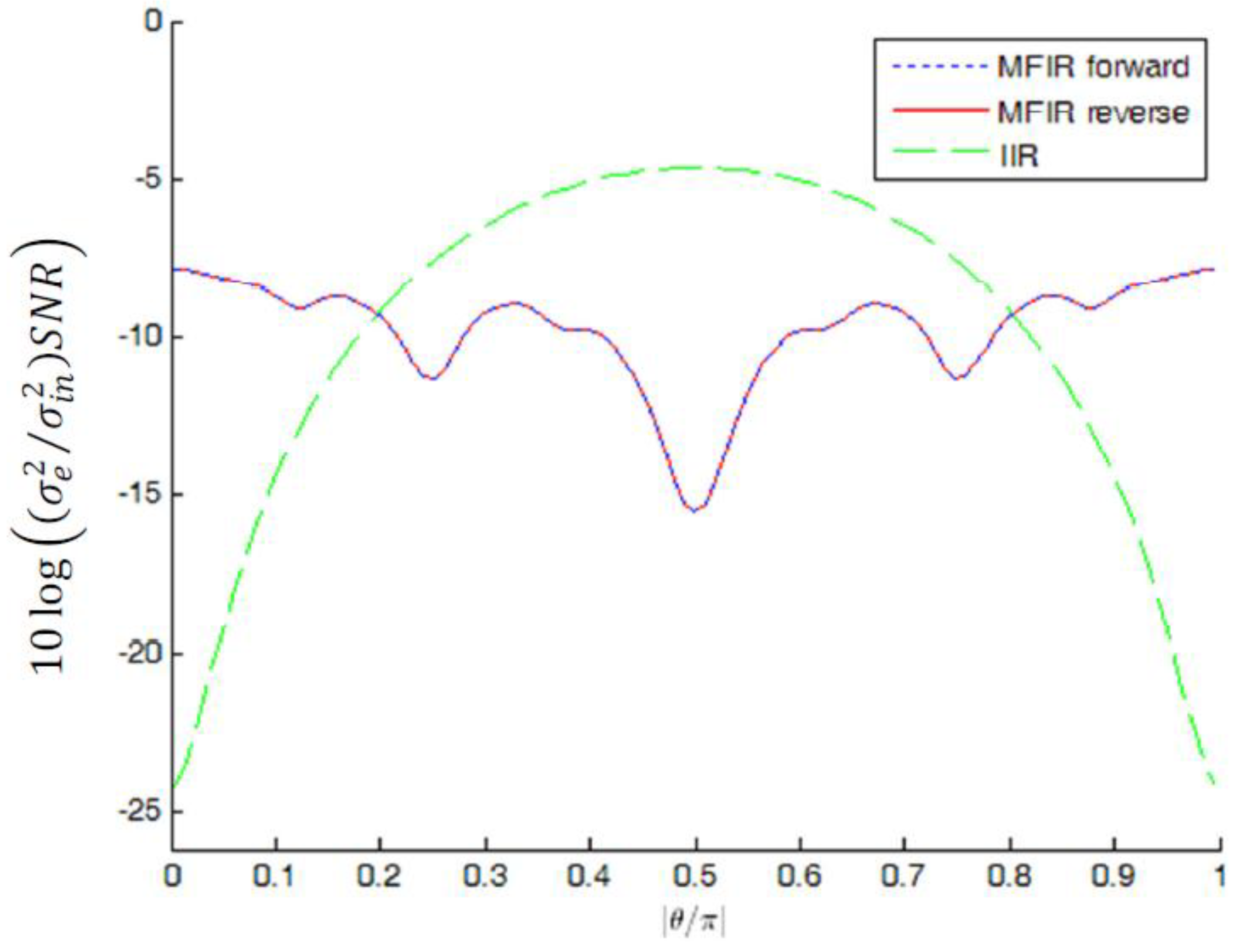
5.3.4. SNR Performance of an MFIR Filter Approximating a Complex-Conjugate Pole Pair Filter in Cascade
values when realizing pole pairs with a magnitude r = 0.9 and angles θ in the interval [0, π) in case of L2 bound scaling. Figure 11 and Figure 12 show the results in case of infinity bound scaling and absolute bound scaling respectively. In Figure 13 the values are calculated for the pole magnitudes: 0.8, 0.85, 0.9 and 0.95 approximated with P = 5, 6, 7, and 7 stages respectively in case of infinity bound scaling and reverse ordering. The surface plots are the values for the MFIR filters. The half circle shaped curves are the values for the corresponding IIR filters. Figure 14 compares the noise performances of the approximation of the complex-conjugate pole pair with a magnitude r = 0.9 and any angle between 0 and π, for several scaling methods and orderings.- is significantly better (up to 20 dB) than the noise performance of its corresponding IIR filter when the approximated poles are situated in the neighborhood of the real axis;
- is far less pole angle θ dependent in comparison with the corresponding IIR filter;
- is up to 2.5 dB better for infinity bound scaling than for absolute bound scaling (using reverse ordering);
- is always better for L2 bound scaling than for the other scaling methods (obeys Equation (44));
- is pole magnitude dependent, but not that much as the corresponding IIR filter;
- is fairly insensitive to an extra MFIR filter stage (typically 1 dB);
- is very sensitive to the stage ordering for absolute and infinity bound scaling;
- is ordering independent in case of L2 bound scaling;
- is in general better in reverse ordering than in forward ordering, except for pole angles in the neighborhood of π/2;
- is for pole angles in the neighborhood of π/2, for absolute and infinity bound scaling, better in forward ordering than in reverse ordering (It was already remarked in Section 4.2, from a theoretical point of view, that this situation could occur.);
- can be up to 6 dB worse than the corresponding IIR filter for pole angles in the neighborhood of π/2. The width of this region and the magnitude of the difference decreases however with increasing pole magnitude ;
5.3.5. SNR Performance of a Linear Phase MFIR filter Approximating the Squared Magnitude Response of a Complex-Conjugate Pole Pair Filter
values for pole pairs with magnitude r = 0.9 and angles θ in the interval [0, π) for forward ordering. Figure 16 shows the values for reverse ordering. In Figure 17, the in case of reverse ordering and infinity bound scaling for the pole magnitudes 0.8, 0.85, 0.9 and 0.95 approximated with P = 5, 6, 7 and 7 stages respectively, is shown. is more pole angle dependent. The dips at the pole angles π/4, π/2 and 3π/4 are also deeper. The figures show that the ordering of the stages has no effect when L2 bound scaling is used. In case of absolute or infinity bound scaling, reverse ordering performs better than forward ordering except in the regions where θ = π/4, π/2, and 3π/4. However, the width of these regions is pole magnitude dependent. Consequently, in practice both orderings will have to be considered when poles with angles in these regions are to be approximated.![Applsci 04 00099 i087]() factors in Equation (5) can have very large values when i is large,
factors in Equation (5) can have very large values when i is large,- cos (2i θ) factors in Equation (5) are for most stages close to unity implying the coefficients are not reduced by the cosine functions.

6. Conclusions
- when approximating a complex-conjugate pole pair having a pole angle in the neighborhood of π/2 and the cascade structure has been used;
- when approximating the squared magnitude response of a complex-conjugate pole pair filter in case the pole angles are situated in the neighborhood of π/4, π/2 and 3π/4 and the linear phase cascade structure has been used.
Conflicts of Interest
References
- Fam, A.T. MFIR filters: Properties and applications. IEEE Trans. Acoust. Speech Signal Process. 1981, 29, 1128–1136. [Google Scholar] [CrossRef]
- Vandenbussche, J.-J.; Lee, P.; Peuteman, J. Analysis of time and frequency domain performance of MFIR filters. In Proceedings of the 2008 International Conference on Embedded Systems and Applications, Las Vegas, NV, USA, 14–17 July 2008; Arabnia, H.R., Mun, Y., Eds.; CSREA Press: Las Vegas, NV, USA, 2008; pp. 323–329. [Google Scholar]
- Rademacher, H. Topics in Analytic Number Theory; Springer Verlag: New York, NY, USA, 1973; Chapter 12; pp. 213–214. [Google Scholar]
- Vandenbusschem, J.-J.; Leem, P.; Peutemanm, J. Linear phase approximation of real and complex pole IIR filters using MFIR structures. In Proceedings of the 5th European Conference on the Use of Modern Information and Communication Technologies, Gent, Belgium, 22–23 March 2012; De Strycker, L., Ed.; Nevelland: Gent, Belgium, 2012; pp. 221–231. [Google Scholar]
- Vandenbussche, J.-J.; Lee, P.; Peuteman, J. An FPGA based digital lock-in amplifier implemented using MFIR resonators. In Proceedings of the International Conference on Signal Processing, Pattern Recognition and Applications, Crete, Greece, 18–20 June 2012; Petrou, M., Sappa, A.D., Triantafyllidis, G.A., Eds.; Acta Press: Calgary, AB, Canada, 2012; Volume 778–034, pp. 92–99. [Google Scholar]
- Vandenbussche, J.-J.; Lee, P.; Peuteman, J. Design of an FPGA based TV-Tuner test bench using MFIR structures. Annu. J. Electron. 2013, 7, 21–25. [Google Scholar]
- Vandenbussche, J.-J.; Lee, P.; Peuteman, J. On the coefficient quantization of multiplicative FIR filters. Digit. Signal Process. 2013, 23, 689–700. [Google Scholar] [CrossRef]
- Jackson, L.B. On the interaction of roundoff noise and dynamic range in digital filters. Bell Syst. Tech. J. 1970, 49, 159–184. [Google Scholar] [CrossRef]
- Chan, D.S.K.; Rabiner, L.R. An algorithm for minimizing roundoff noise in cascade realizations for finite impulse response digital filter. Bell Syst. Tech. J. 1973, 52, 347–385. [Google Scholar] [CrossRef]
- Mitra, S.K. Digital Signal Processing: A Computer-Based Approach, 3rd ed.; Mc Graw Hill Higher Education: New York, NY, USA, 2006; pp. 665–738. [Google Scholar]
- Jackson, L.B. Round-off noise analysis for fixed point digital filters realized in cascade or parallel form. IEEE Trans. Audio Electroacoustics. 1970, 18, 107–122. [Google Scholar] [CrossRef]
- Chan, D.S.K.; Rabiner, L.R. Analysis of quantization errors in the direct form for finite impulse response digital filters. IEEE Trans. Audio Electroacoustics. 1973, 21, 354–366. [Google Scholar] [CrossRef]
- Fettweis, A. Roundoff noise and attenuation sensitivity in digital filters with fixed-point arithmetic. IEEE Trans. Circuit Theory 1973, 20, 174–175. [Google Scholar] [CrossRef]
- Mondal, K.; Mitra, S.K. Roundoff noise upper bounds for cascaded recursive digital filter structures. IEE Proc. Electron. Circuit Syst. 1982, 129, 250–256. [Google Scholar] [CrossRef]
- Lim, Y.C.; Liu, B. Design of cascade form FIR filters with discrete valued coefficients. IEEE Acoust. Speech Signal Process. 1988, 36, 1735–1739. [Google Scholar] [CrossRef]
- Montgomery Smith, L.; Henderson, M.E. Roundoff noise reduction in cascade realizations of FIR digital filters. IEEE Trans. Signal Process. 2000, 48, 1196–2000. [Google Scholar] [CrossRef]
- Dehner, G.F. Noise optimized IIR digital filter design-tutorial and some new aspects. Signal Process. 2003, 83, 1565–1582. [Google Scholar] [CrossRef]
- Shi, D.; Yu, Y.J. Design of discrete-valued linear phase FIR filters in cascade form. IEEE Trans. Circuits Syst. 2011, 58, 1627–1636. [Google Scholar] [CrossRef]
- Vandenbussche, J.-J. Analysis and Implementation of MFIR Filters in FPGA Technology. Ph.D. Thesis, University of Kent, Canterbury, UK, September 2012. [Google Scholar]
© 2014 by the authors; licensee MDPI, Basel, Switzerland. This article is an open access article distributed under the terms and conditions of the Creative Commons Attribution license (http://creativecommons.org/licenses/by/3.0/).
Share and Cite
Vandenbussche, J.-J.; Lee, P.; Peuteman, J. Round-Off Noise of Multiplicative FIR Filters Implemented on an FPGA Platform. Appl. Sci. 2014, 4, 99-127. https://doi.org/10.3390/app4020099
Vandenbussche J-J, Lee P, Peuteman J. Round-Off Noise of Multiplicative FIR Filters Implemented on an FPGA Platform. Applied Sciences. 2014; 4(2):99-127. https://doi.org/10.3390/app4020099
Chicago/Turabian StyleVandenbussche, Jean-Jacques, Peter Lee, and Joan Peuteman. 2014. "Round-Off Noise of Multiplicative FIR Filters Implemented on an FPGA Platform" Applied Sciences 4, no. 2: 99-127. https://doi.org/10.3390/app4020099
APA StyleVandenbussche, J.-J., Lee, P., & Peuteman, J. (2014). Round-Off Noise of Multiplicative FIR Filters Implemented on an FPGA Platform. Applied Sciences, 4(2), 99-127. https://doi.org/10.3390/app4020099