A Far-Field Helicopter Acoustic Detection Method Based on FRESH Adaptive Filtering

Abstract

Helicopter detection plays a vital role in obtaining critical aerial information promptly and ensuring the safety of lives and property. Since a helicopter’s aerodynamic noise primarily consists of main rotor noise, the cyclostationarity of this noise becomes our detection target. This paper proposes a filter based on the Frequency-Shift (FRESH) principle, which is updated using the Adam optimization algorithm. A smoothed global detector is presented to detect the cyclic frequency of rotor noise. The effectiveness of the proposed helicopter detection approach, comprising both the filter and the detector, has been validated through simulations and confirmed by far-field experiments with a ROBINSON R22 helicopter. In these tests, the proposed method was compared against a cyclostationarity adaptive filter based on the Normalized Least Mean Squares (NLMS) algorithm, as well as the traditional Detection of Envelope Modulation on Noise (DEMON) and Cyclic Modulation Coherence (CMC) algorithms. Experimental results demonstrate the superior robustness of the proposed method over these benchmarks. Even at extended ranges between 11 and 13 km, the system retains a consistent detection rate of 77.8%.

1. Introduction

Helicopters are vital in military and civilian fields, making their detection essential for low-altitude security. Since the emergence of helicopters in the early 20th century, detection technology has been continuously evolving. Traditionally, helicopter detection has relied on active detection technologies such as radar detection [1,2]. However, since radar systems were originally designed for fixed-wing aircraft, they often perform poorly when carrying out helicopter detection missions. Due to the low flight altitude and slow speed of helicopters, coupled with the interference of rotor blade echoes, radar echoes are often weak and subject to interference. Given these challenges and the unique noise characteristics generated by rotors, passive detection of helicopter acoustic signals has become an important alternative or supplement to traditional radar systems.

The noise of helicopters mainly comes from components such as the main rotor, tail rotor, engine, and fuselage. Despite the presence of numerous noise sources, the aerodynamic noise generated by the rotor dominates the overall sound pressure level. Therefore, existing studies typically use the aerodynamic noise level of the rotor as the standard for evaluating the overall acoustic impact of the helicopter [3,4,5,6].

Existing research on acoustic helicopter detection primarily focuses on rotor noise analysis [7,8,9,10,11]. Due to the limitations of experimental conditions, the measurement of rotor noise is usually carried out in a simulated environment, such as a silencing wind tunnel. To better simulate the acoustic detection and noise analysis scenarios in the real world, outdoor research on actual helicopter flights is considered more effective. Ground microphone arrays are usually used for far-field data acquisition, although they will face the challenges of SNR and environmental interference [12].

Researchers have developed passive detection systems by taking advantage of the acoustic characteristics of helicopters [13,14]. Most current methods prioritize harmonic characteristics. Yet, detecting these signals proves difficult because the main rotor’s tonal noise overlaps significantly with low-frequency environmental clutter. The rotational motion of rotor blades produces modulated aerodynamic noise, amenable to demodulation techniques such as DEMON (Detection of Envelope Modulation on Noise) [15], spectral kurtosis (SK) [16,17], and cyclostationary analysis [18,19]. However, DEMON relies on extensive experience, while SK struggles to identify precise frequency bands under low-SNR conditions for reliable results [20,21].

The theory of cyclostationarity was first proposed by William A. Gardner [22]. Cyclostationary signals are a special class of non-stationary random signals whose statistical properties vary periodically with time. Cyclostationary analysis is a method used to process signals with periodic statistical properties and is widely applied in fields such as communication signal processing, mechanical fault diagnosis, and target detection [23,24]. In reference [25], Z. Lin first introduced cyclostationary analysis to detect helicopter aerodynamic noise. However, in this paper, he only considered the first-order cyclostationary features and did not address far-field helicopter detection under strong interference conditions. Subsequently, L. Yu et al. investigated second-order cyclostationary characteristics of rotor signals and developed a model for helicopter rotor aerodynamic noise [26]. Cyclostationary analysis can extend the detection range of helicopters in low-SNR far-field scenarios. Angle-time cyclostationary analysis has been applied to isolate tonal and broadband noise components from counter-rotating open rotors [27,28].

Building on the cyclostationary properties of helicopter rotor noise, frequency-shift (FRESH) filtering emerges as a powerful technique for exploiting spectral correlation to remove interference and enhance signal detection in low-SNR environments [29]. Originally introduced for cyclostationary signals in communication systems, FRESH filters shift frequencies to align periodic components, offering advantages over traditional time-invariant filters like Wiener filters, particularly in rejecting noise from radar or communication signals [30]. This approach has been extended to time-varying variants for handling almost cyclostationary signals with non-commensurate cyclic frequency, as demonstrated in applications involving pulsed radar chirps [31].

In recent years, the field of aerial acoustic detection has seen significant advancements, particularly driven by data-driven approaches. Comprehensive reviews have highlighted the evolution from classical signal processing to modern deep learning techniques for Unmanned Aerial Vehicle and helicopter detection [32,33]. For instance, lightweight Convolutional Neural Networks (CNNs) and residual networks (ResNet) have been successfully applied to extract robust acoustic features from complex environmental noise, achieving high recognition accuracy [34]. Parallel to these learning-based methods, research into modern cyclostationary detection continues to evolve. Recent studies have demonstrated that combining machine learning classifiers with acoustic features—such as Mel-frequency cepstral coefficients (MFCCs) and cyclostationary signatures—can further enhance detection performance in low-SNR conditions [35]. However, while deep learning models offer impressive detection rates, they typically require large-scale annotated datasets and substantial computational resources, which may not always be available for specific helicopter targets in far-field scenarios. Therefore, adaptive filtering methods that explicitly exploit the physical cyclostationarity of rotor noise, such as the FRESH filter proposed in this work, remain a critical and efficient solution.

We propose a filter that combines the Adam optimizer [36] used in machine learning to accelerate gradient descent with the FRESH filter. This process starts with the Fast Spectral Correlation (FAST-SC) technology and is based on the Short-Time Fourier Transform (STFT) [37] for detecting the cyclic frequency. Subsequently, the obtained spectral features are used to construct the frequency-shifted version of the input signal of the FRESH filter. After obtaining the filtered signal, we construct a global detector to determine whether the filtered signal is the aerodynamic noise of the helicopter. The primary contributions of this work are as follows:

• By combining the Adam optimizer with the FRESH filter framework, a FRESH filter suitable for far-field helicopter sound detection was constructed. Unlike general frequency domain filters, this filter is designed to filter the cyclic frequencies of non-stationary signals with periodic characteristics, such as helicopter rotor noise.
• A global detector for multiple cyclic frequencies was designed to determine whether the signal filtered by FRESH is the aerodynamic noise of a helicopter. The global detector can adaptively calculate the statistical threshold while taking into account the random jitter of the cycle frequency.

The remainder of this paper is organized as follows. Section 2 describes the structure of the proposed FRESH adaptive filter. Section 3 presents an adaptive detection strategy. Section 4 validates both the filtering method and the detection strategy through simulations, with performance compared against the NLMS-based FRESH filter. Section 5 applies the entire detection method to a far-field helicopter experiment. Section 6 discusses the results and limitations. Finally, Section 7 provides the conclusions.

To ensure mathematical consistency and clarity throughout the paper, the key notations and parameters used in the proposed method are summarized in

Table 1. List of key notations and parameters.

Symbol	Description
L	Filter order (length of the coefficients)
N	Number of filter branches (cyclic frequencies)
i	Harmonic index ($i=1,\dots ,n$)
${\alpha }_k$	The k-th cyclic frequency
$x\left(t\right)$	Input signal
$y\left(t\right)$	Ideal reference signal
$\widehat{y}\left(t\right)$	Output of the FRESH filter
$S{C}_{2p}(\alpha ,f)$	Spectral coherence density
$G\left(\alpha \right)$	Detection indicator
$p_i$	Local peak within the i-th harmonic band
${\lambda }_{1-p_{fa}}$	Statistical threshold for a given false alarm rate
$Q_i$	Local quality score for the i-th harmonic
Q	Global detection score
$\theta$	Normalized decision threshold

.

2. FRESH Adaptive Filtering

2.1. Spectral Coherence Estimation

According to cyclostationary theory, a signal $x\left(t\right)$ is first-order cyclostationary if its ensemble average varies periodically. The tonal noise $P_{tonal}\left(t\right)$ is proven to be a first-order cyclostationary signal [26] and thus has an ensemble periodical average $m_p\left(t\right)$:

$$m_p\left(t\right)=\mathbb{E}\left\{P_{tonal}\left(t\right)\right\}=m_p(t+kT),$$

(1)

where $\mathbb{E}\left\{\right\}$ denotes the ensemble average, and T is the period.

A signal is second-order cyclostationary if its autocorrelation function varies periodically. The modulated broadband noise $p_b\left(t\right)$ due to blade rotation exhibits this property and is proven to be second-order cyclostationary [26]:

$$R_{2p}(t,\tau )=\mathbb{E}\left\{p_b(t+\tau /2)p_b^{*}(t-\tau /2)\right\}=R_{2p}(t+kT,\tau ),$$

(2)

Here, $\tau$ corresponds to the time delay variable, and the superscript * indicates the complex conjugate operation. The cyclic autocorrelation function $R_{2p}^{\alpha }$ is the Fourier series coefficient of $R_{2p}(t,\tau )$:

$$R_{2p}({\alpha }_k,\tau )={\displaystyle \frac{1}{T}}{\int }_{-T/2}^{T/2}{R}_{2p}(t,\tau )e^{-j2\pi {\alpha }_{k}t}dt$$

(3)

where ${\alpha }_k$ is the cyclic frequency of the kth. The spectral correlation density (SCD) $S_{2p}({\alpha }_k,f)$ is the Fourier transform of $R_{2p}({\alpha }_k,f)$:

$$S_{2p}({\alpha }_k,f)={\int }_{-\infty }^{\infty }{R}_p({\alpha }_k,f)e^{-j2\pi f\tau }d\tau =\mathbb{E}\left\{P_b(f+{\alpha }_k/2)P_b^{*}(f-{\alpha }_k/2)\right\},$$

(4)

where f represents the spectral frequency, while $P_b$ denotes the frequency-domain representation of the broadband noise component $p_b$. It characterizes how the signal’s power is distributed relative to the spectral frequency f at each specific cyclic frequency ${\alpha }_k$.

To address scaling effects in SCD that may obscure minor features under strong interference, the spectral coherence $S{C}_{2p}({\alpha }_k,f)$ provides a normalized method:

$$S{C}_{2p}({\alpha }_k,f)={\displaystyle \frac{cor{r}_{2p}(f+{\alpha }_k/2,f-{\alpha }_k/2)}{\sqrt{P(f+{\alpha }_k/2)P(f-{\alpha }_k/2)}}}={\displaystyle \frac{S_{2p}({\alpha }_k,f)}{\sqrt{S_{2p}(0,f+{\alpha }_k/2)S_{2p}(0,f-{\alpha }_k/2)}}}$$

(5)

where the term ${\mathrm{corr}}_{2p}$ denotes the autocorrelation in the frequency domain.

Traditional methods usually rely on fast approximation (FAM) [38]. However, considering the influence of FAM on noise and non-stationarity [39], the Fast-SC technique [37] was adopted in this study. This method is based on STFT and provides excellent stability in complex signal environments.

2.2. The Structure of FRESH Adaptive Filter

Unlike traditional filters, the FRESH filter excels in separating noise and signals with spectral overlap, making it a key technology for suppressing interference. Its operation is based on the cyclostationary theory, which holds that periodic statistical changes will generate predictable correlations among the distant spectral lines. We utilize the spectral correlation coefficient to quantify this redundancy, enabling the system to take advantage of the frequency-shifted signal version to achieve enhanced sensitivity in far-field applications with low SNR.

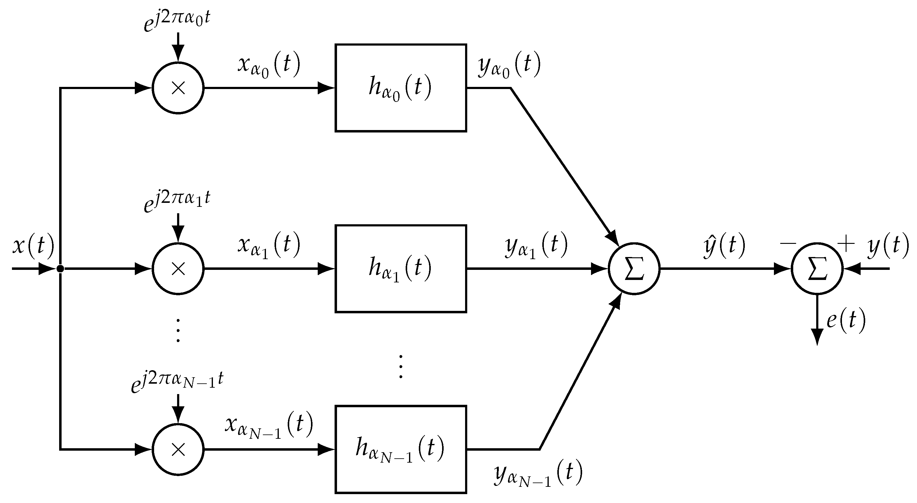
When $S{C}_{2p}=0$, the two spectral components are completely uncorrelated, indicating no redundancy between the components at frequencies $f+\alpha /2$ and $f-\alpha /2$. In contrast, $S{C}_{2p}=1$ signifies full correlation and complete spectral redundancy, where the components are linearly dependent, allowing one to cancel or recover the other. For cyclic signals, the spectral components at $f+\alpha /2$ and $f-\alpha /2$ are correlated. Based on this mechanism, we adopt the LMS criterion for helicopter aerodynamic noise and propose a filter structure as shown in Figure 1.

$x\left(t\right)$ represents the single-channel signal from an individual microphone; in our experiments, this corresponds to the audio captured by the center microphone of the array. $x_{a_i}\left(t\right)$ is a frequency-shifted version of $x\left(t\right)$, where the shift amounts ${\alpha }_0,\dots ,{\alpha }_{N-1}$ are obtained using the Fast-SC algorithm. The ideal signal $y\left(t\right)$ is acquired from close-range measurements of helicopter rotor noise with a high SNR. We can obtain the output $\widehat{y}\left(t\right)$:

$${\widehat{y}}_{{\alpha }_i}\left(n\right)=\sum _{k=0}^{L-1}{h}_{{\alpha }_i}\left(k\right)x_{{\alpha }_i}(n-k)={\mathbf{h}}_{{\alpha }_i}^{\mathrm{T}}{\mathbf{x}}_{{\alpha }_i}\left(n\right)$$

(6)

where

$${\mathbf{h}}_{{\alpha }_i}=\left(\begin{array}{c}{h}_{{\alpha }_i}\left(0\right)\\ h_{{\alpha }_i}\left(1\right)\\ ⋮\\ h_{{\alpha }_i}(L-1)\end{array}\right){\mathbf{x}}_{{\alpha }_i}\left(n\right)=\left(\begin{array}{c}{x}_{{\alpha }_i}\left(n\right)\\ x_{{\alpha }_i}(n-1)\\ ⋮\\ x_{{\alpha }_i}(n-L+1)\end{array}\right),$$

and $x_{{\alpha }_i}\left(k\right)=x\left(k\right)e^{j2\pi {\alpha }_{i}k}$.

The total output is

$$\widehat{y}\left(n\right)=\sum _{i=1}^N{\widehat{y}}_{{\alpha }_i}\left(n\right)=\sum _{i=1}^N{\mathbf{h}}_{{\alpha }_i}^{†}{\mathbf{x}}_{{\alpha }_i}\left(n\right)={\mathbf{H}}^{†}\mathbf{x}\left(n\right),$$

(7)

where

$$\mathbf{X}\left(n\right)={\left[{\mathit{x}}_{{\alpha }_1}^T\left(n\right){\mathit{x}}_{{\alpha }_2}^T\left(n\right)\cdots {\mathit{x}}_{{\alpha }_N}^T\left(n\right)\right]}^T,$$

(8)

$${\mathbf{H}}^{†}\left(n\right)=\left[{\mathit{h}}_{{\alpha }_1}^{†}{\mathit{h}}_{{\alpha }_2}^{†}\cdots {\mathit{h}}_{{\alpha }_N}^{†}\right],$$

(9)

† denotes the conjugate transpose. And the constraint equation is given by the following expression:

$$\begin{array}{cc}\hfill \underset{\mathbf{h}\left(n\right)}{\min }& \mathcal{L}\left(n\right)={\left|e\left(n\right)\right|}^2,\hfill \\ \hfill \mathrm{s}.\mathrm{t}.& e\left(n\right)=y\left(n\right)-\widehat{y}\left(n\right)=y\left(n\right)-{\mathbf{h}}^{†}\left(n\right)\mathbf{x}\left(n\right).\hfill \end{array}$$

(10)

In practical far-field detection scenarios, a synchronized ideal reference signal $y\left(n\right)$ is not always available. However, the proposed FRESH filter can operate in a blind adaptive mode by utilizing the received signal $x\left(n\right)$ itself as the reference (i.e., replacing $y\left(n\right)$ with $x\left(n\right)$ in Equation (10)).

This approach exploits the spectral redundancy of cyclostationary signals. The target helicopter noise exhibits strong correlation between its spectral components at frequencies f and $f+\alpha$, whereas the stationary environmental noise does not. Consequently, when the filter weights are updated to minimize the error between the output and the noisy input $x\left(n\right)$, the algorithm selectively preserves the cyclostationary components that are correlated with the frequency-shifted inputs ${\mathbf{x}}_{\alpha }\left(n\right)$ while suppressing the uncorrelated stationary noise. This mechanism ensures the robustness of the detector even without a clean reference signal.

The proposed FRESH filter is updated using the Adam algorithm [36]. Instead of a single, fixed step size, Adam computes an individual, adaptive learning rate for each filter weight. This is achieved by maintaining exponentially decaying averages of past gradients (first-order moment) and their squared magnitudes (second-order moment).

The update for the filter weight vector ${\mathbf{h}}_{{\alpha }_i}\left(n\right)$ of the i-th branch is performed as follows:

$${\mathbf{h}}_{{\alpha }_i}(n+1)={\mathbf{h}}_{{\alpha }_i}\left(n\right)+{\delta }_{{\alpha }_i}\left(n\right),$$

(11)

where ${\delta }_{{\alpha }_i}\left(n\right)$ is the adaptive update vector calculated by Adam at time step n. The calculation of ${\delta }_{{\alpha }_i}\left(n\right)$ involves the following steps.

First, compute the gradient vector ${\mathbf{g}}_{{\alpha }_i}\left(n\right)$ with respect to the filter weights ${\mathbf{h}}_{{\alpha }_i}\left(n\right)$:

$${\mathbf{g}}_{{\alpha }_i}\left(n\right)=e\left(n\right)·{\mathbf{x}}_{{\alpha }_i}^{*}\left(n\right),$$

(12)

where ${\mathbf{x}}_{{\alpha }_i}^{*}\left(n\right)$ is the conjugate of the input signal vector corresponding to the weight vector ${\mathbf{h}}_{{\alpha }_i}\left(n\right)$.

Update the first-order moment ${\mathbf{m}}_{{\alpha }_i}\left(n\right)$ (moving average of the gradient) and the second-order moment ${\mathbf{v}}_{{\alpha }_i}\left(n\right)$ (moving average of the squared gradient magnitude):

$$\begin{array}{cc}\hfill {\mathbf{m}}_{{\alpha }_i}\left(n\right)& ={\beta }_1·{\mathbf{m}}_{{\alpha }_i}(n-1)+(1-{\beta }_1)·{\mathbf{g}}_{{\alpha }_i}\left(n\right),\hfill \\ \hfill {\mathbf{v}}_{{\alpha }_i}\left(n\right)& ={\beta }_2·{\mathbf{v}}_{{\alpha }_i}(n-1)+(1-{\beta }_2)·{\left|{\mathbf{g}}_{{\alpha }_i}\left(n\right)\right|}^2,\hfill \end{array}$$

(13)

where ${\beta }_1$ and ${\beta }_2$ are exponential decay rates, typically 0.9 and 0.999, respectively.

Adjust the first and second moment estimates to compensate for the error caused by the initial 0:

$$\begin{array}{cc}\hfill {\widehat{\mathbf{m}}}_{{\alpha }_i}\left(n\right)& ={\displaystyle \frac{{\mathbf{m}}_{{\alpha }_i}\left(n\right)}{1-{\beta }_1^n}},\hfill \\ \hfill {\widehat{\mathbf{v}}}_{{\alpha }_i}\left(n\right)& ={\displaystyle \frac{{\mathbf{v}}_{{\alpha }_i}\left(n\right)}{1-{\beta }_2^n}}.\hfill \end{array}$$

(14)

In the final step, the adaptive update term ${\delta }_{{\alpha }_i}\left(n\right)$ is formulated by using the modified moment estimation. This vector replaces the traditional scalar step size update:

$${\delta }_{{\alpha }_i}\left(n\right)=\mu ·{\displaystyle \frac{{\widehat{\mathbf{m}}}_{{\alpha }_i}\left(n\right)}{\sqrt{{\widehat{\mathbf{v}}}_{{\alpha }_i}\left(n\right)}+ϵ}},$$

(15)

where $\mu$ represents the basic learning rate, and $ϵ$ denotes the numerical stability term added to avoid division by zero errors (usually ${10}^{-8}$).

3. Multi-Cyclic Frequency Peak Detection Approach

The helicopter acoustic signal passing through the FRESH filter has more distinct cyclic spectral peaks. Based on this, we propose a global detector for detecting multi-cycle spectral peaks. This global detector detects helicopter rotor noise that overlaps with noise on the spectrum by detecting multiple cyclic frequencies [40].

3.1. Problem Statement

The helicopter acoustic signal collected by the microphone $x\left(t\right)$ consists of two parts, the rotor noise $p\left(t\right)$ and environmental noise $n\left(t\right)$:

$$x\left(t\right)=p\left(t\right)+n\left(t\right).$$

(16)

Our goal is to detect rotor noise as much as possible, even if the characteristic harmonic features are severely damaged due to spectral interference. Therefore, we mathematically represent the detection problem within the framework of binary hypothesis testing:

$$\left\{\begin{array}{c}{\mathcal{H}}_0:d\left(n\right)=n\left(t\right)\hfill \\ {\mathcal{H}}_1:d\left(n\right)=p\left(t\right)+n\left(t\right),\hfill \end{array}\right.$$

(17)

where $d\left(n\right)$ represents the collected acoustic signal, ${\mathcal{H}}_0$ indicates that the collected acoustic signal is pure background noise, and ${\mathcal{H}}_1$ indicates that the collected acoustic signals are rotor noise and background noise.

This paper constructs specific detection statistics to perform binary hypothesis testing. Under the preset false alarm probability $p_{fa}$, by comparing this statistic with the decision threshold, it is determined whether to reject the null hypothesis ${\mathcal{H}}_0$.

3.2. Construction of the Detection Function

For robust far-field rotor noise identification, we formulate a detection index derived from the FRESH filter output $\widehat{y}\left(n\right)$. By utilizing the inherent cyclostationarity, the method effectively distinguishes the target signal from the environmental background noise, ensuring superior performance even in low-SNR environments.

Referring to the definition in Section 2.1, spectral coherence ${\widehat{SC}}_x(\alpha ,f)$ is used to standardize the cyclic spectrum. Therefore, we define the detection indicator $G\left(\alpha \right)$ as the integral of the spectral coherence over the frequency band B:

$$G\left(\alpha \right)={\int }_B∥{\widehat{SC}}_x(\alpha ,f)∥df\approx \mathrm{\Delta }f\sum _{f\in B}∥{\widehat{SC}}_x(\alpha ,f)∥,$$

(18)

where $\mathrm{\Delta }f$ is the frequency resolution. This is the basis of the hypothesis test in the Equation (17). The detection threshold ${\lambda }_{1-p_{fa}}$ is adaptively set by the percentile method, corresponding to the expected false alarm rate $p_{fa}$. This dynamic method ensures a constant false alarm rate (CFAR) under different noise conditions.

To account for rotor speed variations and Doppler shifts, search bands $R_i$ are defined around the i-th harmonic $i·{\alpha }_1$ (where ${\alpha }_1$ is the fundamental BPF):

$$\begin{array}{cc}\hfill {\alpha }_i^L& =(1-\delta )·i·{\alpha }_1\hfill \\ \hfill {\alpha }_i^U& =(1+\delta )·i·{\alpha }_1\hfill \\ \hfill B_i& =\left[{\alpha }_i^L,{\alpha }_i^U\right],\hfill \end{array}$$

(19)

where the factor $\delta$ determines the relative width of the search band. For example, the value $\delta =0.05$ corresponds to the search range ±5% near the theoretical harmonic frequency. This design ensures that the system can adapt to the subtle changes in the speed of the helicopter’s rotor during flight.

To identify the most significant response within the i-th harmonic band, the detection function $G\left({\alpha }_k\right)$ is evaluated across all candidate cyclic frequencies ${\alpha }_k$. The local peak $p_i$ is

$$p_i=\underset{{\alpha }_k\in B_i}{max}G\left({\alpha }_k\right).$$

(20)

The local quality score $Q_i$ for the i-th harmonic is

$$Q_i=\left\{\begin{array}{cc}{\displaystyle \frac{p_i-{\lambda }_{1-p_{fa}}}{p_i}}\hfill & p_i\ge {\lambda }_{1-p_{fa}},\hfill \\ 0\hfill & p_i<{\lambda }_{1-p_{fa}}.\hfill \end{array}\right.$$

(21)

The global detection score Q, fusing n harmonics, is

$$Q={\displaystyle \frac{1}{n}}\sum _{i=1}^n{Q}_i.$$

(22)

This Q score serves as an indicator for determining whether there are harmonic characteristics consistent with the rotor noise. To establish a comparative reference, calculate another statistic: the average amplitude of all spectral points that exceed the threshold ${\lambda }_{1-p_{fa}}$, denoted as $AM$:

$$AM={\displaystyle \frac{{\sum }_{k=1}^{k_{max}}G\left({\alpha }_k\right)·{\mathbf{1}}_{G\left({\alpha }_k\right)>{\lambda }_{1-p_{fa}}}}{N_b}},$$

(23)

where $N_b$ is the count of points on the entire cycle frequency axis that exceed ${\lambda }_{1-p_{fa}}$. The normalized threshold $\theta$ is

$$\theta ={\displaystyle \frac{AM-{\lambda }_{1-p_{fa}}}{AM}}.$$

(24)

Whenever the global probability score Q exceeds the threshold $\theta$, we assume that the target feature exists and supports hypothesis ${\mathcal{H}}_1$. If this threshold is not reached, the assumption ${\mathcal{H}}_0$ is supported. Although the instantaneous check $Q\left(q\right)>\theta \left(q\right)$ can provide immediate results for each window q, it is still vulnerable to the influence of instantaneous noise peaks. This type of artifact is usually manifested as isolated false positives, lacking the persistence of the real target. Therefore, we implemented the time post-processing module. This step utilizes the continuity of the helicopter’s acoustic characteristics to filter out occasional errors.

First, a binary decision sequence, $D\left(q\right)$, is generated from the instantaneous results:

$$D\left(q\right)=\left\{\begin{array}{cc}1,\hfill & \mathrm{if}Q\left(q\right)\ge \theta \left(q\right)\hfill \\ 0,\hfill & \mathrm{otherwise}\hfill \end{array}\right.$$

(25)

We pass the original detection results through a sliding window moving average filter, a time-smoothing technique designed to filter out transient noise spikes while maintaining the continuity of real helicopter features. The final robust determination $D_s\left(q\right)$ depends on the density of positive markers within a window of width w. Only when the local proportion exceeds the confirmation ratio $\gamma$ do we consider the target to exist ($D_s\left(q\right)=1$):

$$D_s\left(q\right)=\left\{\begin{array}{cc}1,\hfill & \mathrm{if}{\displaystyle \frac{1}{w}}\sum _{k=q-w/2}^{q+w/2-1}D\left(k\right)\ge \gamma \hfill \\ 0,\hfill & \mathrm{otherwise}\hfill \end{array}\right.$$

(26)

where w determines the duration of the time integral, while the scalar $\gamma$ serves as a proportional threshold, constrained by the interval $(0,1]$. The specific implementation steps of the proposed multi-cyclic frequency detection method are summarized in Algorithm 1.

Algorithm 1: Proposed Multi-Cyclic Frequency Detection Algorithm

By implementing this post-processing logic, we can suppress false alarms caused by instantaneous environmental noise, thereby protecting the true acoustic characteristics of the target. Each test result analyzed in this study is derived from this smoothed decision flow D_s(q).

4. Simulation

4.1. Simulation Signal Model and Experiment Setup

The effectiveness of the proposed method for detecting helicopter aerodynamic noise is validated through simulations. The simulated signal is modeled based on the cyclostationary properties of rotor noise, following the approach in [40], as expressed below.

$$p\left(t\right)=\underset{\mathrm{tonal}\mathrm{noise}}{\underbrace{\sum _i{A}_{i}cos2\pi f_{SF}t+\sum _i{B}_{i}cos2\pi f_{BF}t}}+\underset{\mathrm{broadband}\mathrm{noise}}{\underbrace{\left[1+\sum _i{A}_{i}cos2\pi f_{SF}t+\sum _i{B}_{i}cos2\pi f_{BF}t\right]·c\left(t\right),}}$$

(27)

where

• $f_{SF},f_{BF}$ represent the shaft rotation frequency (SRF) and the blade passing frequency (BPF) of the main rotor, respectively;
• $A_i,B_i$ represent the amplitudes of the ith components of SRF and BPF;
• $c\left(t\right)$ represents the stationary carrier of the broadband noise.

The synthesized signal model, incorporating additive noise, is thus given by

$$x\left(t\right)=p\left(t\right)+n\left(t\right).$$

(28)

To simulate the aerodynamic noise characteristics of the main rotor of a real helicopter, the key simulation parameters of the rotor shaft and the main rotor are shown in

Table 2. Simulation parameters of the helicopter main rotor.

Simulation Parameter	Parameter Layout
Sample frequency/kHz	51.2
Number of blades	4
Rotating speed/rpm	2051
$f_{SF}$/Hz	34.2
$f_{BF}$/Hz	136.8
i	15
$A_i$	$0.2/i$
$B_i$	$1/i$
$c\left(t\right)$	Gaussian white noise

. These parameters ensure the true periodic stability characteristics and are suitable for adaptive filtering analysis.

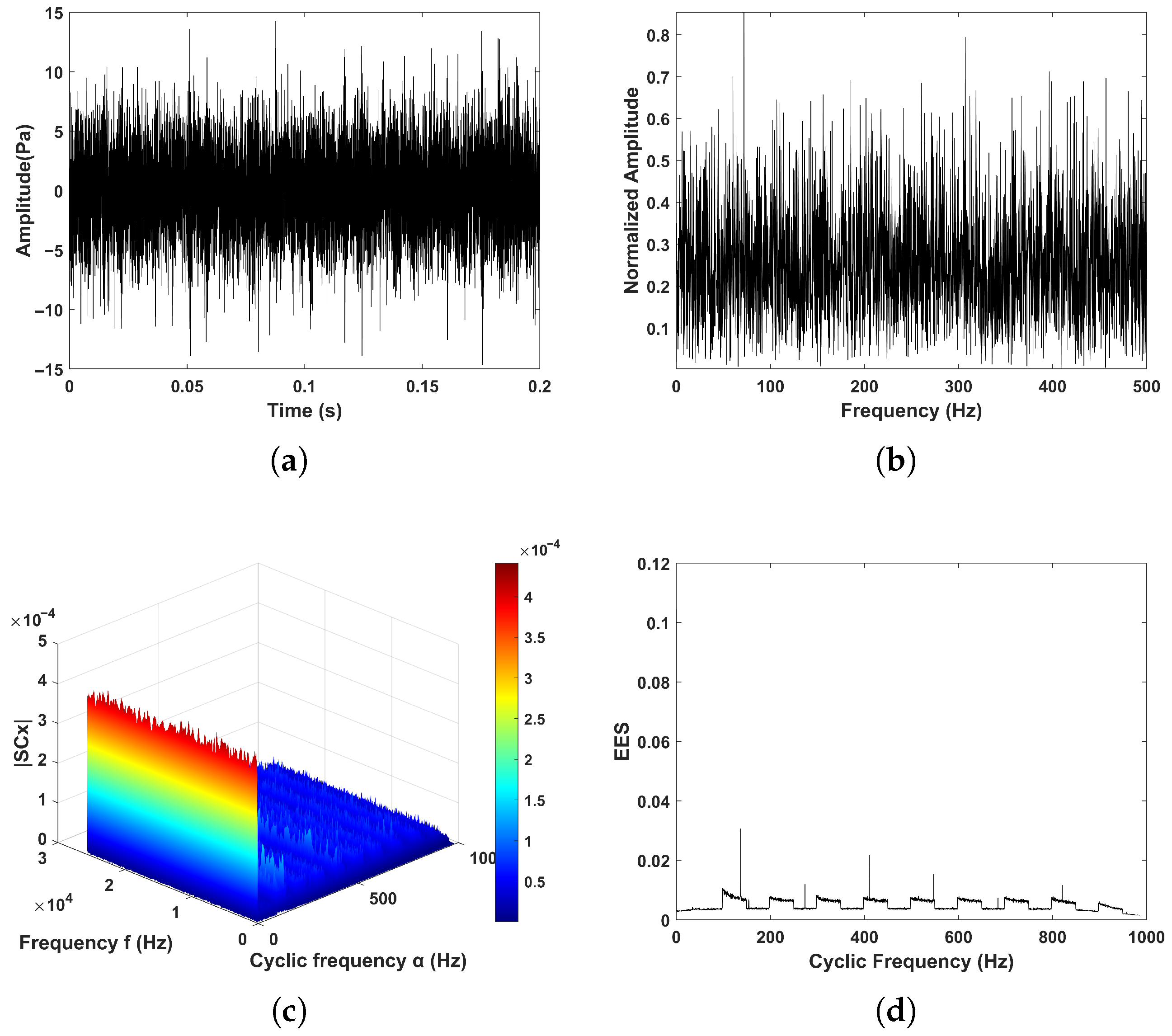
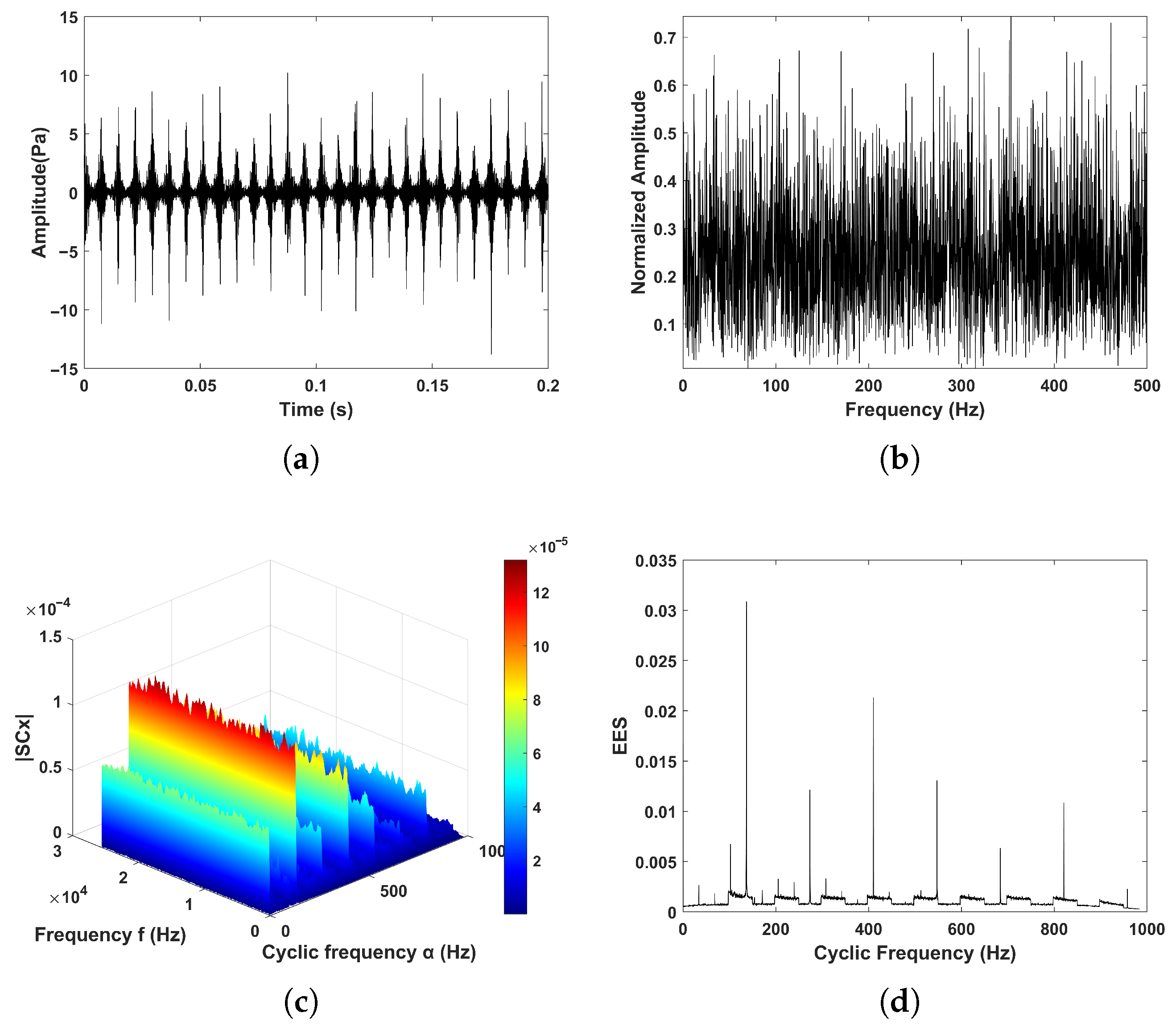
We applied the Fast-SC algorithm to estimate spectral coherence using a Hamming window of length $N_w=512$ with $95\%$ overlap. The FFT size was set to $N_{fft}=512$. The method was tested under two conditions: a noise-free signal and a noisy signal with an SNR of $-10$ dB. Figure 2 and Figure 3 present the respective time-domain waveforms and spectral coherence density plots. Specifically, panel (d) in each figure displays the mean density averaged along the spectral-frequency axis. While the noise-free spectrum (Figure 2) clearly reveals spectral lines corresponding to the cyclic frequency components, these features become obscured in the $-10$ dB case (Figure 3) due to significant Gaussian white noise interference.

4.2. Filtering and Performance Evaluation

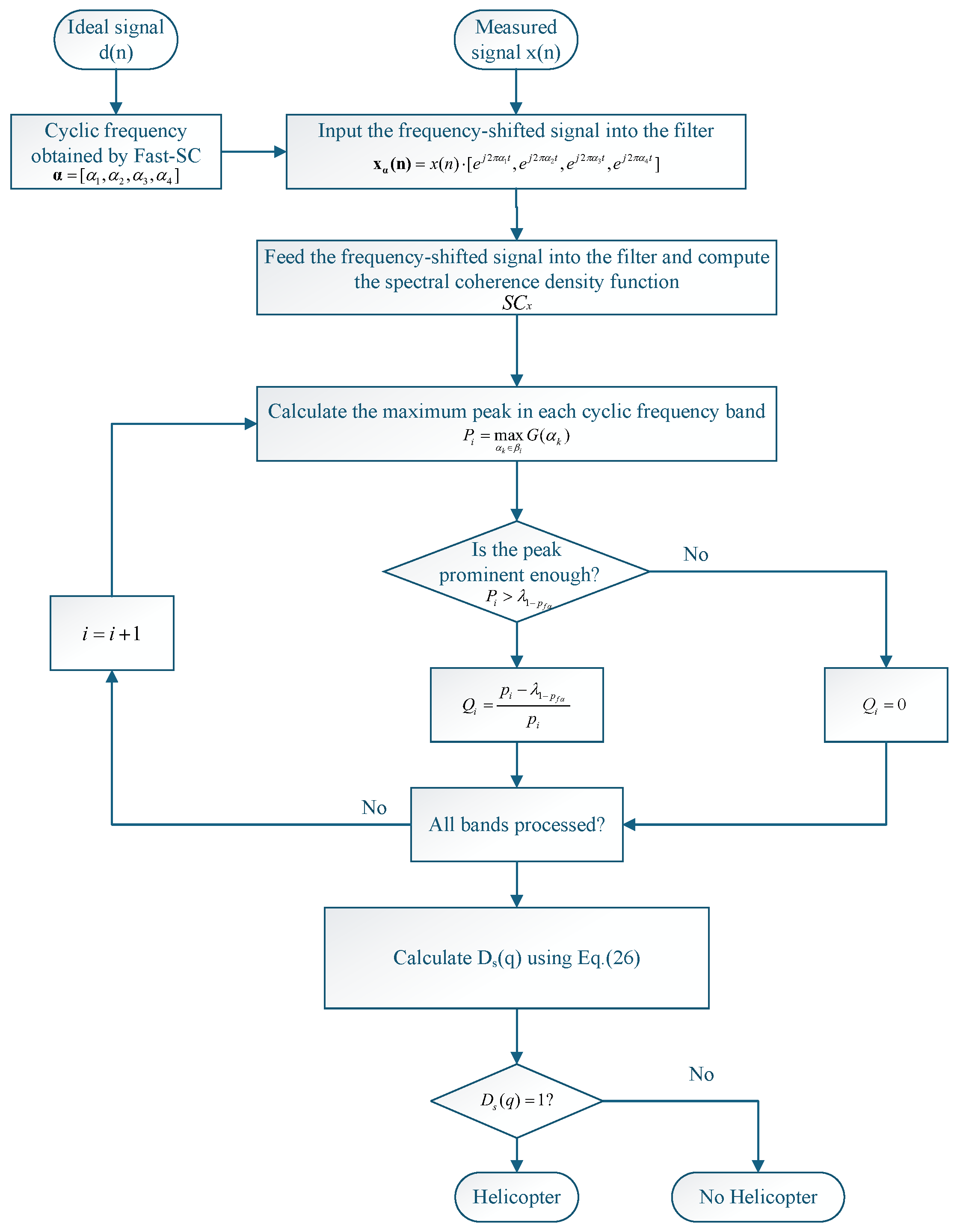
The FRESH adaptive filter is used to process simulated signals with SNRs ranging from $-20$ dB to 0 dB. The signals are generated using the model in Equation (27), with parameters as specified in Table 2. The frequency offsets $\alpha$ for the filter inputs are selected as the first four prominent cyclic frequencies from Figure 2d, namely $\mathbf{\alpha }=[136.866,273.532,410.398,547.265]\mathrm{Hz}$. The filtered output undergoes cyclic spectral analysis to compute the spectral coherence $S{C}_x$, which is then input to the proposed detector for helicopter detection. The complete filtering-detection workflow is depicted in Figure 4.Where the calculation formula for the EES is given by

$$EES\left(\alpha \right)={\int }_{f_1}^{f_2}S{C}_x(f,\alpha )df$$

(29)

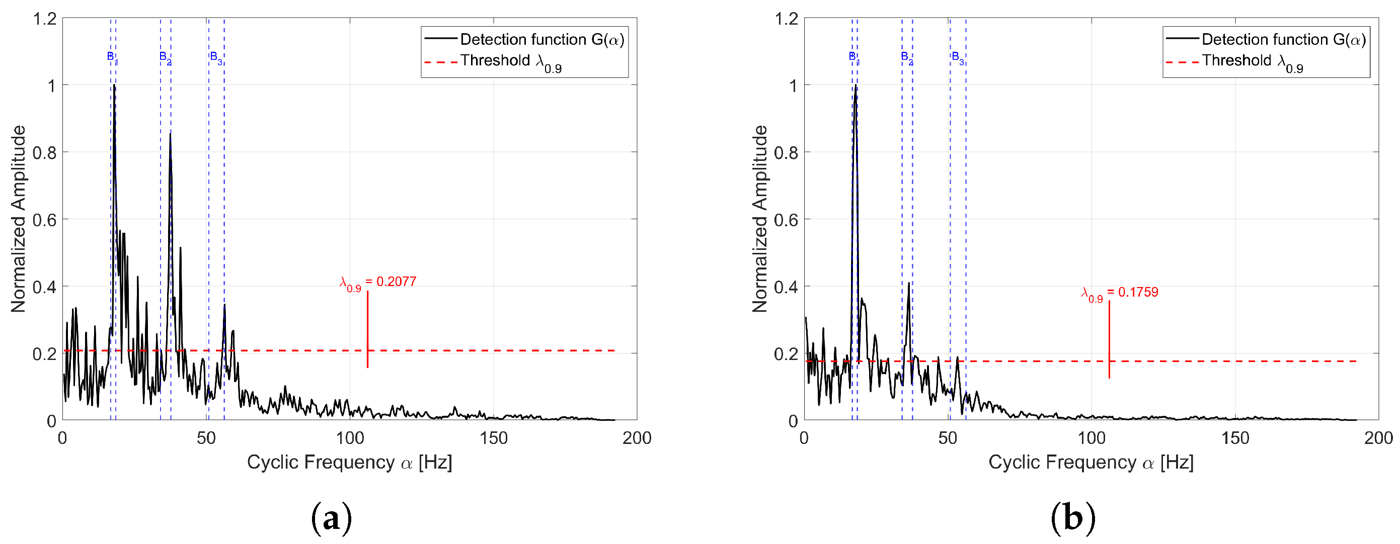
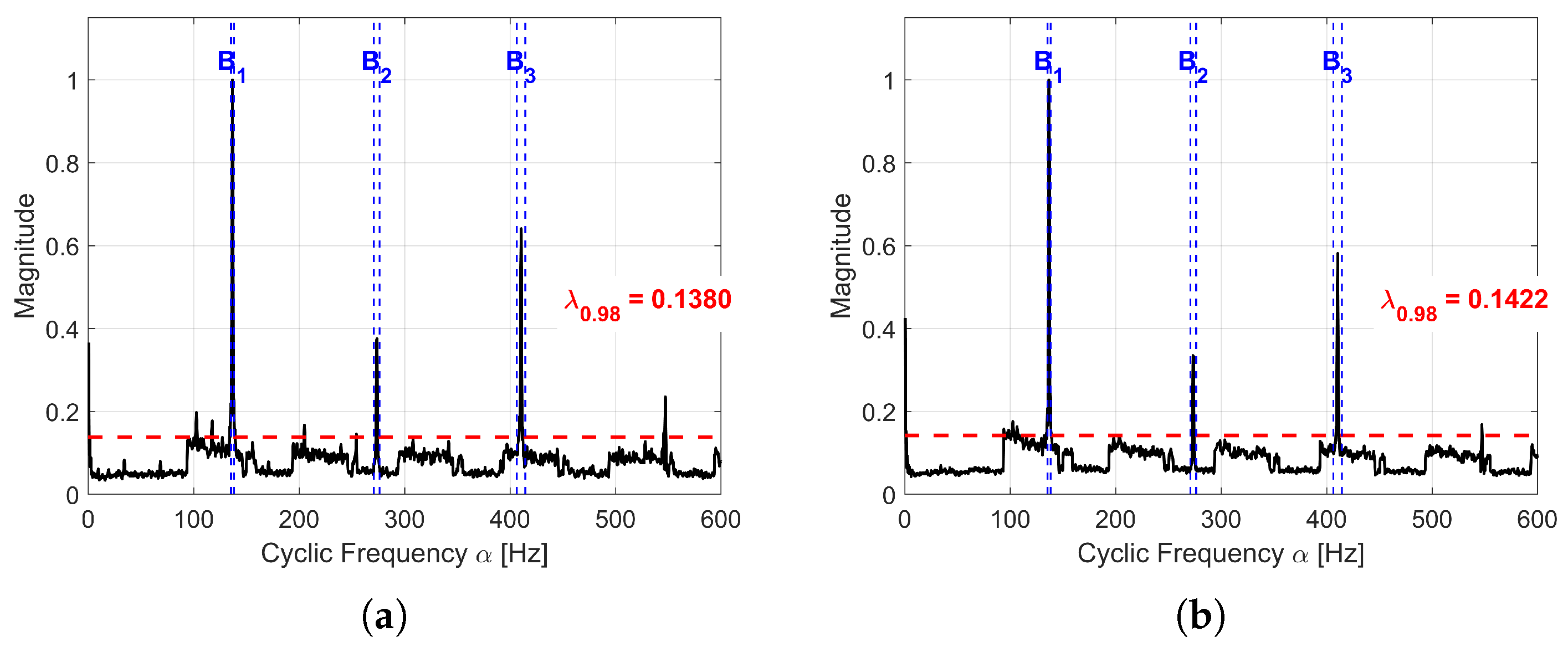
As illustrative examples, consider signals with SNRs of −1 dB and −5 dB. For SNR = −1 dB (Figure 5a), the detection threshold ${\lambda }_{p_{fa}}$ is set with $p_{fa}=0.02$, yielding ${\lambda }_{p_{fa}}=0.138$. The detector identifies three cyclic frequencies, with corresponding detection bands $B_1=[135.308,138.042]$ Hz, $B_2=[270.617,276.085]$ Hz, and $B_3=[406.424,414.634]$ Hz. The relationship between the detection function G and the threshold ${\lambda }_{p_{fa}}$ shows three distinct cyclic spectral peaks, and the computed indicator $G=0.4922$ exceeds the threshold $\theta =0.4794$, confirming successful detection. Similarly, for the signal with SNR = −5 dB as shown in Figure 5b, the threshold ${\lambda }_{p_{fa}}=0.1422$, and the global score $Q=0.4435$ also exceeds the threshold $\theta =0.4213$. It indicates that the detector can detect helicopter noise in both cases.

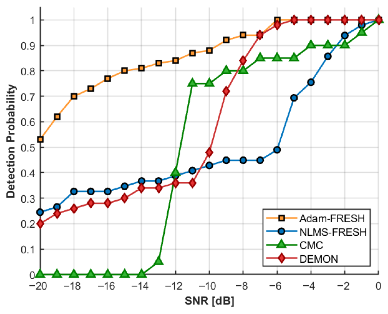
We evaluated the detection performance of the proposed FRESH filter using the Adam optimizer across an SNR range of $-20\mathrm{dB}$ to $0\mathrm{dB}$. For comparison, we benchmarked it against the FRESH filter using the NLMS algorithm, as well as the traditional CMC and DEMON algorithms. As shown in Figure 6, the detection probabilities for these four methods are presented under varying SNR conditions.

The simulation results indicate that the FRESH adaptive filter utilizing the Adam optimizer consistently outperforms the NLMS variant, as well as the CMC and DEMON algorithms, throughout the range from $-20\mathrm{dB}$ to $0\mathrm{dB}$. This performance advantage is particularly evident in the low-SNR region ($-20\mathrm{dB}$ to $-12\mathrm{dB}$), where the Adam-FRESH filter maintains significantly higher detection probabilities while traditional methods exhibit sharp degradation. Although the CMC algorithm shows a steep performance jump around $-13\mathrm{dB}$ and surpasses the NLMS filter in the moderate SNR range, it remains inferior to the Adam–FRESH filter. The DEMON algorithm generally requires higher SNR levels for reliable detection compared to the other methods. The superior robustness of the Adam–FRESH filter is attributed to Adam’s momentum-based adaptive learning rates, making it highly suitable for low-SNR applications in acoustic detection systems.

5. Experiment

5.1. Experimental Arrangement

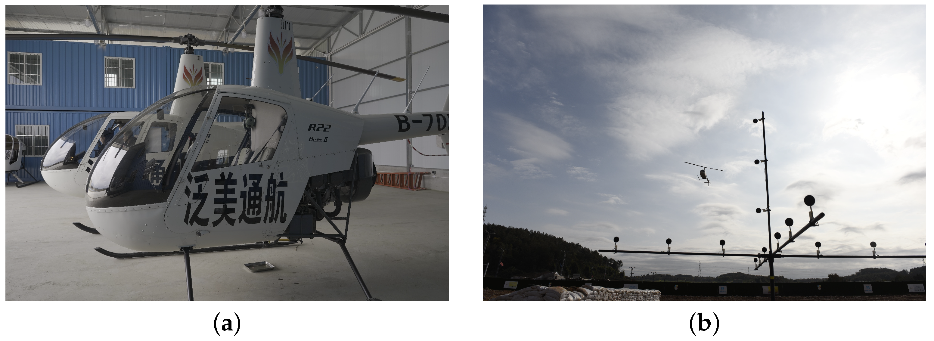
To verify the efficacy of the suggested detection scheme, a far-field flight trial was carried out in Mianyang, Sichuan Province, China. The test involved a ROBINSON R22 helicopter, as illustrated in Figure 7a, which is a light utility helicopter equipped with a two-bladed main rotor.

A cross-shaped microphone array was deployed in an open test field to capture acoustic signals, as shown in Figure 7b. The array consisted of 1/4-inch G.R.A.S. 46 BD pressure microphone sets arranged with a spacing of 0.5 m between adjacent sensors. These microphones feature a frequency range of $4\mathrm{Hz}$ to $100\mathrm{kHz}$, a dynamic range of $35\mathrm{dB}$ to $160\mathrm{dB}$, and a nominal sensitivity of $4\mathrm{mV}/\mathrm{Pa}$. To minimize wind noise interference during the experiment, windscreens were attached to all microphones as depicted in the figure.

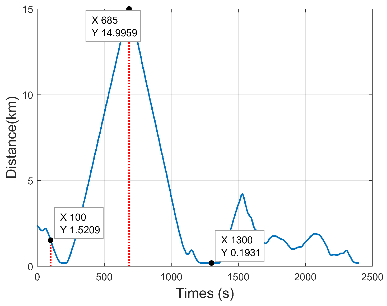
During the experiment, the helicopter took off near the microphone array, flew away to a maximum distance, and then returned, maintaining a flight altitude of approximately 50 m relative to the ground. The test lasted for approximately 2400 s, and the helicopter achieved a maximum distance of about 15 km at approximately 685 s. Considering that the rotor harmonics are mainly below 200 Hz, the data was recorded at a sampling rate of 5000 Hz, which conforms to the Nyquist sampling law to ensure no signal distortion. A Global Positioning System (GPS) was employed to track and record the real-time distance between the helicopter and the microphone array. For the handheld GPS, the Real-Time Kinematic (RTK) accuracy was 2.5 cm ± 1 ppm (tracking sensitivity −158 dBm), while the differential positioning device’s RTK accuracy was 1.5 cm ± 1 ppm. The measured range profile is illustrated in Figure 8, where the X-axis represents the time elapsed since the start of the experiment, and the Y-axis denotes the distance between the helicopter and the microphone array. The detailed list of experimental devices is shown in

Table 3. Experimental devices.

Measurement Equipment	Amount	Purpose
Data acquisition host computer	1	Running the helicopter acoustic detection data acquisition and processing software.
Controller/power box	1	Data acquisition equipment control and power supply.
Data acquisition equipment	9	Controlling microphones to capture noise/data relay.
Microphone array frame	9	Supporting and mounting the microphones.
Array transmission cable	9	Equipment power supply and signal transmission.
Microphone	9 × 15	Acquiring noise signals.
Dedicated mobile hard disk	1	Data storage.
Handheld GPS device	1	Recording helicopter position.
Differential positioning device	1	Recording the position of the microphone array.

.

5.2. Cyclic Frequency Detection

The primary objective of the cyclic adaptive filter is to enhance signals exhibiting specific, known cyclic frequencies. Therefore, the initial critical step involves accurately identifying the characteristic cyclic frequencies of the helicopter’s rotor noise. To accomplish this, a signal segment captured under high SNR conditions is analyzed to determine the target frequencies for the filter.

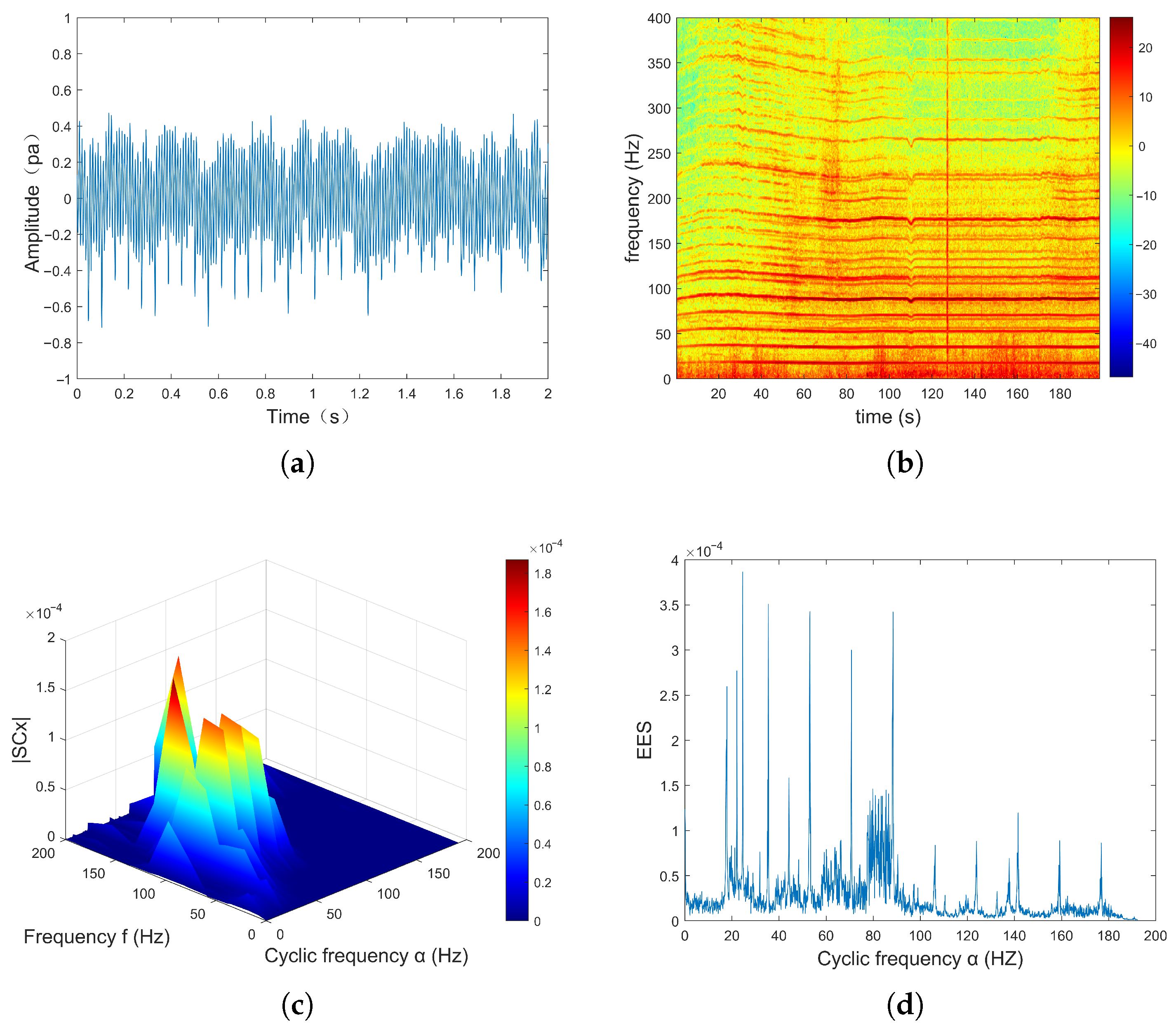
To investigate the cyclic spectral characteristics of the helicopter noise, a signal segment at 1300 s was selected, corresponding to a scenario where the helicopter was positioned at a close distance of 0.193 km from the microphone array. At this proximity, the signal strength is high and environmental interference is minimal, providing an ideal baseline for feature extraction.

The Fast-SC algorithm was applied to this 10-s data segment. The analysis parameters were configured as follows: a Hamming window was employed to mitigate spectral leakage, with the window length set to $N_w=256$. To ensure high resolution in the cyclic frequency domain and capture fine temporal variations, a window overlap of $95\%$ was utilized for the STFT calculation.

The resulting spectral coherence density is illustrated in Figure 9. Spectral inspection isolates a sequence of sharp peaks attributed to the rotor’s acoustic footprint. We pinpoint the fundamental Blade Passage Frequency (BPF) at ${\alpha }_1\approx 17.724$ Hz, accompanied by clearly defined higher-order harmonics: the second, third, and fourth. Leveraging these features, we initialize the cyclic adaptive filter with the frequency vector $\mathit{\alpha }=[17.724,35.446,53.173,70.896]$ Hz. Unless otherwise specified, this frequency vector and the aforementioned windowing parameters are consistently applied to all subsequent experimental analyses in this chapter.

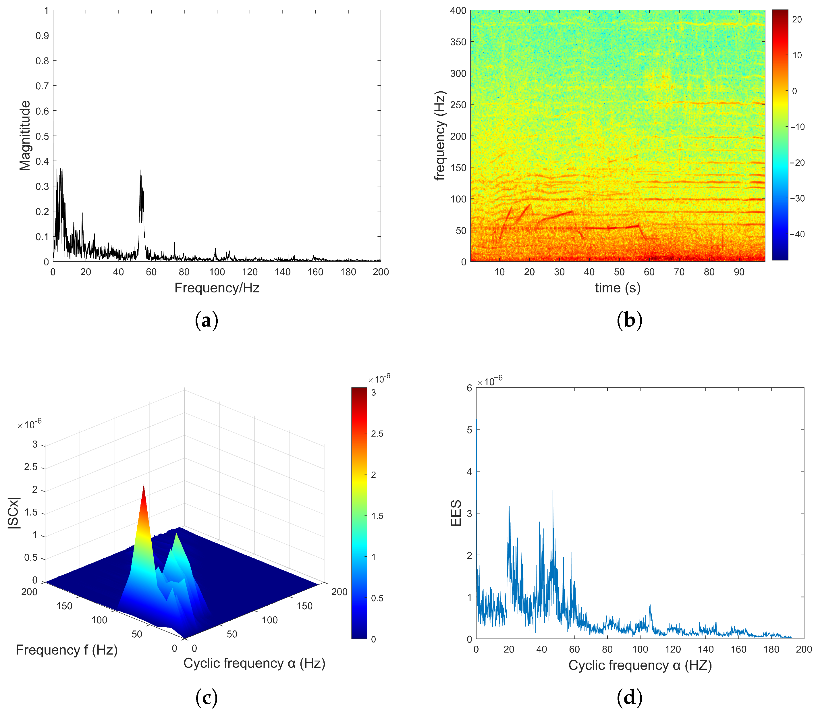
As a comparison, Figure 10 shows the spectral analysis of the helicopter at a distance of approximately 4 km at 1000 s. In this case, due to the significant attenuation of the helicopter’s noise energy, the target’s cyclic frequency signal is submerged in the background noise. This energy loss indicates that direct spectral analysis is not effective at long distances. To overcome this limitation, we adopted the proposed cyclic adaptive filter to extract the weak signals embedded in the noise by targeting the predetermined modulation frequency.

5.3. Cyclic Adaptive Filtering

We verified the effectiveness of the proposed FRESH filter using the Adam optimizer through actual far-field experiments. Therefore, the complete 2400 s acoustic dataset of the flight test was processed through two different optimization strategies: the Adam algorithm and the standard NLMS method. The filter parameters are configured as follows: filter order L = 32, cyclic frequencies $\mathit{\alpha }=[17.724,35.446,53.173,70.896]$ Hz (corresponding to the fundamental BPF and its first three harmonics), Adam hyperparameters ${\beta }_1=0.9$, ${\beta }_2=0.999$, $ϵ=1\times {10}^{-8}$, and initial learning rate $\mu =0.001$, and NLMS step size $\mu =0.001$. These settings take advantage of the cyclic frequency of rotor noise and ensure numerical stability.

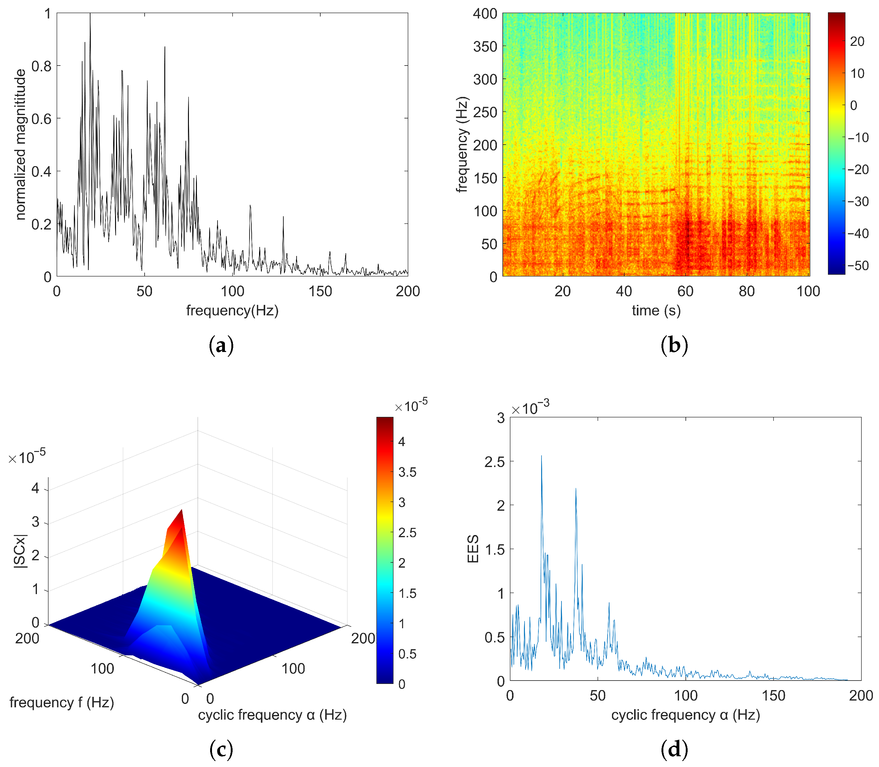
To evaluate the performance under low-SNR conditions, we selected data ranging from 185 s to 1085 s. The 900 s data represented the sound signal collected by the microphone of the helicopter when it reached a maximum distance of about 15 km and flew back to the nearest 200 m at approximately 685 s. The filtered frequency-domain spectra in Figure 11a confirm the effectiveness of this method: The FRESH filter extracts periodic rotor components, providing a spectrum characterized by sharp peaks in EES. Figure 11c shows the spectral coherence density of the noise after filtering. The resulting spectrum features sharp and distinct peaks located at specific cycle frequencies. This clarity validates the filter’s ability to restore and amplify weak cyclic stationary patterns masked by environmental noise.

5.4. Detection

To verify the overall effectiveness of the framework, we input both the 900 s filtered far-field helicopter data and the 400 s pure background noise recording from the previous text into our global detector and post-processing logic. Before filtering, we standardized all signals through normalization to ensure amplitude consistency.

We demonstrated the effect of the detector using the results of passing through the filter and detector in 1000 s (4 km) and 385 s (5 km). The frequency shift version of the signal used requires the cycle frequencies obtained from spectral estimation of the signal at approximately 200 m: 17.724, 35.446 and 53.173 Hz. Figure 12 shows the relationship between the detection function and the threshold $\lambda$. For a 1000 s sample, the global metric Q reaches 0.5834, safely exceeding the decision threshold $\theta$ of 0.3913. Similarly, at 385 s, the value of Q was 0.4866, also exceeding the required threshold of 0.4178. Therefore, the system recorded valid detection results in both of these instances.

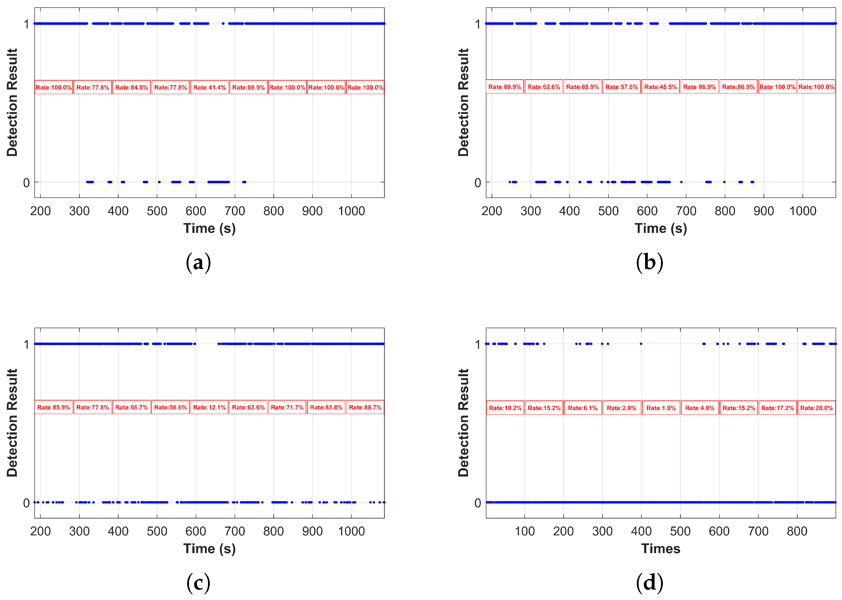
To comprehensively evaluate the performance of the proposed method, we conducted a comparative experiment involving the FRESH filter based on the Adam optimizer, the FRESH filter based on NLMS, the classic DEMON algorithm, and the CMC algorithm. The detection results were computed at 100 s intervals, and the comparisons are presented in Figure 13.

The results indicate significant differences in detection capabilities among the four algorithms. The CMC algorithm (Figure 13d) exhibited the poorest performance under the experimental conditions, with detection rates generally below 20%, failing to effectively extract the target signal. In contrast, while the DEMON algorithm and the NLMS-based FRESH filter showed improved performance, they still suffered from considerable fluctuations during low SNR periods. The FRESH filter utilizing the Adam optimizer (Figure 13a) demonstrated a distinct advantage, maintaining the highest detection rates and stability across most time intervals. This result aligns with the simulation findings, confirming that the Adam-based FRESH filter offers superior robustness and detection performance compared to CMC, DEMON, and traditional NLMS algorithms in far-field acoustic detection scenarios.

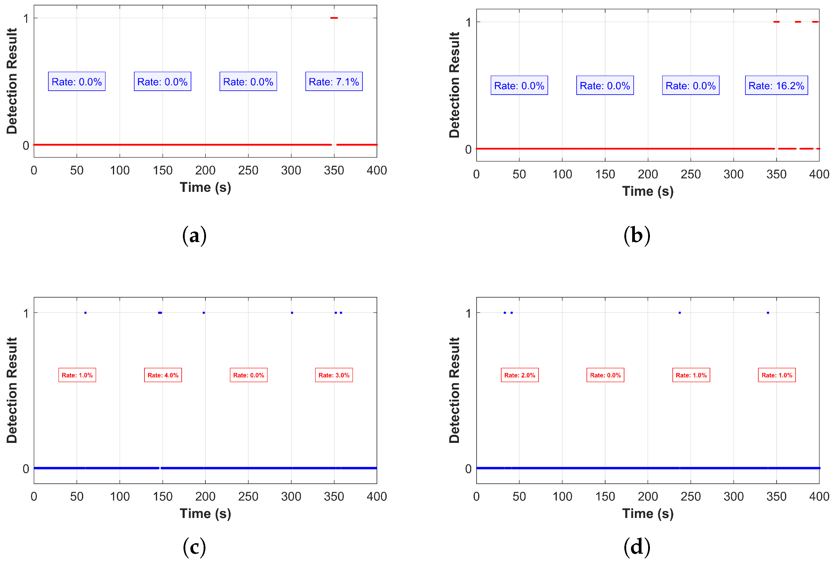
Additionally, 400 s of background noise were collected and processed using the same procedure to evaluate the detector’s false alarm rate under a CFAR design of 10%. False alarm rates were computed at 100 s intervals. The results for background noise using the proposed Adam-optimized FRESH filter, the NLMS-based FRESH filter, the DEMON algorithm, and the CMC algorithm are presented in Figure 14a, b, c, and d, respectively.

Notably, the false alarm rates remain at 0% across the 0–300 s interval for both the Adam-optimized and NLMS-based filters. In the 300–400 s interval, the false alarm rate is 7.1% for the Adam-optimized filter, compared to 16.2% for the NLMS-based filter. In contrast, the DEMON algorithm (Figure 14c) exhibits sporadic false alarms throughout the recording, with rates ranging from 0.0% to 4.0% in different intervals. Similarly, the CMC algorithm (Figure 14d) shows consistent low-level false alarms, ranging between 0.0% and 2.0%. These results demonstrate that the proposed filtering and detection framework maintains a superior low false alarm rate profile under pure noise conditions while achieving a detection rate of 77.8% at a distance of 11–13 km.

6. Discussion

Both simulation and experimental results show that the proposed FRESH filter based on Adam optimization performs effectively under far-field conditions. The helicopter signal achieved a detection rate of 77.8% when detected at distances from 11 km to 13 km, maintaining a relatively low false alarm rate under a constant false alarm rate design of 10%. In comparison, the traditional CMC algorithm exhibited limited effectiveness in these far-field scenarios, with detection rates generally falling below 20%. Similarly, the DEMON algorithm required higher SNR for reliable detection and suffered from performance fluctuations. Specifically, for background noise, the false alarm rate of the proposed method remains at 0% within the 0–300 s range, and it is 7.1% within the 300–400 s range. In contrast, the NLMS-based filter exhibits a significantly higher false alarm rate of 16.2% in the same interval. The overall false alarm rate of the Adam optimization method is 4.02%, indicating that it possesses higher robustness and lower volatility in low-SNR far-field acoustic environments compared to the NLMS algorithm.

However, the FRESH filter shows sensitivity in the selection of the cycle frequency. In the experiment, the helicopter’s return flight towards the microphone array introduced a Doppler frequency shift, causing a deviation in the estimated cycle frequency and thereby reducing the detection performance. In future work, the Doppler frequency shift can be calculated to achieve more accurate cyclic frequency estimation, which may enhance the adaptability of filters in dynamic electronic detection systems.

7. Conclusions

Due to signal attenuation, detecting the rotor noise of helicopters at a long distance is a well-known difficult problem. To address this issue, our research proposes a detection method that utilizes the characteristics of cyclostationary signals. This architecture combines the FRESH adaptive filter and the Adam optimizer, providing a solution suitable for low-SNR environments. To further enhance reliability, the global detector adopts a smooth operation of multi-cycle frequency detection, effectively suppressing false alarms.

To verify the practical effectiveness, this study compared the proposed method with the FRESH filter using NLMS algorithm, as well as the traditional DEMON and CMC algorithms. Verification relies on simulation data and real far-field acoustic records obtained from ROBINSON R22 flight tests. During the flight test, the FRESH filter optimized by Adam successfully extracted the key cycle frequency features, achieving a detection rate of 77.8% from 11 km to 13 km while maintaining a low false alarm rate.

References

1. Monakov, A. Radar detection and recognition of a hovering helicopter. In Proceedings of the 2021 Wave Electronics and Its Application in Information and Telecommunication Systems (WECONF), St. Petersburg, Russia, 31 May–4 June 2021; IEEE: New York, NY, USA, 2021; pp. 1–7. [Google Scholar]
2. Misiurewicz, J.; Kulpa, K.S.; Czekala, Z.; Filipek, T.A. Radar detection of helicopters with application of CLEAN method. IEEE Trans. Aerosp. Electron. Syst. 2012, 48, 3525–3537. [Google Scholar] [CrossRef]
3. Schmitz, F.H. The Challenges and Possibilities of a Truly Quiet Helicopter 29th Alexander A. Nikolsky Honorary Lecture. J. Am. Helicopter Soc. 2016, 61, 041001. [Google Scholar] [CrossRef]
4. George, A.R. Helicopter noise: State-of-the-art. J. Aircr. 1978, 15, 707–715. [Google Scholar] [CrossRef]
5. Lowson, M.; Ollerhead, J. A theoretical study of helicopter rotor noise. J. Sound Vib. 1969, 9, 197–222. [Google Scholar] [CrossRef]
6. Yang, Y.; Pröbsting, S.; Liu, Y.; Zhang, H.; Li, C.; Li, Y. Effect of dual vortex shedding on airfoil tonal noise generation. Phys. Fluids 2021, 33, 075102. [Google Scholar] [CrossRef]
7. Yu, L.; Wu, H.; Antoni, J.; Jiang, W. Extraction and imaging of aerodynamically generated sound field of rotor blades in the wind tunnel test. Mech. Syst. Signal Process. 2019, 116, 1017–1028. [Google Scholar] [CrossRef]
8. Yu, L.; Gong, Z.; Chu, N.; Ning, Y.; Zheng, Y.; Hou, P. Adaptive imaging of sound source based on total variation prior and a subspace iteration integrated variational Bayesian method. IEEE Trans. Instrum. Meas. 2021, 70, 1–17. [Google Scholar] [CrossRef]
9. Guo, Y.; Zhou, Y.; Guan, L.; Bao, M. Acoustic helicopter recognition via convolutional neural network. In Proceedings of the 2018 IEEE 23rd International Conference on Digital Signal Processing (DSP), Shanghai, China, 19–21 November 2018; IEEE: New York, NY, USA, 2018; pp. 1–5. [Google Scholar]
10. Greenwood, E.; Schmitz, F.H. A parameter identification method for helicopter noise source identification and physics-based semiempirical modeling. J. Am. Helicopter Soc. 2018, 63, 1–14. [Google Scholar] [CrossRef]
11. Chu, N.; Ning, Y.; Yu, L.; Liu, Q.; Huang, Q.; Wu, D.; Hou, P. Acoustic source localization in a reverberant environment based on sound field morphological component analysis and alternating direction method of multipliers. IEEE Trans. Instrum. Meas. 2021, 70, 1–13. [Google Scholar] [CrossRef]
12. Greenwood, E.; Schmitz, F.H. Separation of main and tail rotor noise from ground-based acoustic measurements. J. Aircr. 2014, 51, 464–472. [Google Scholar] [CrossRef]
13. Damarla, T.R.; Ufford, D. Helicopter detection using harmonics and seismic-acoustic coupling. In Proceedings of the Unattended Ground, Sea, and Air Sensor Technologies and Applications X, Orlando, FL, USA, 6–20 March 2008; SPIE: Bellingham, WA, USA, 2008; Volume 6963, pp. 259–264. [Google Scholar]
14. Akhtar, S.; Elshafei-Abmed, M.; Ahmed, M.S. Detection of helicopters using neural nets. IEEE Trans. Instrum. Meas. 2001, 50, 749–756. [Google Scholar] [CrossRef]
15. Lee, J.H.; Han, J.M.; Park, H.G.; Seo, J.S. Application of signal processing techniques to the detection of tip vortex cavitation noise. J. Hydrodyn. 2013, 25, 440–449. [Google Scholar] [CrossRef]
16. Antoni, J. Fast computation of the kurtogram for the detection of transient faults. Mech. Syst. Signal Process. 2007, 21, 108–124. [Google Scholar] [CrossRef]
17. Lee, J.H.; Seo, J.S. Application of spectral kurtosis to the detection of tip vortex cavitation noise. Mech. Syst. Signal Process. 2013, 40, 222–236. [Google Scholar] [CrossRef]
18. Antoni, J.; Hanson, D. Detection of surface ships from interception of cyclostationary signature with the cyclic modulation coherence. IEEE J. Ocean. Eng. 2012, 37, 478–493. [Google Scholar] [CrossRef]
19. Gao, Y.; Cain, T.; Cooper, P. Automatic detection of underwater propeller signals using cyclostationarity analysis. Mech. Syst. Signal Process. 2021, 146, 107032. [Google Scholar] [CrossRef]
20. Antoni, J.; Randall, R.B. The spectral kurtosis: Application to the vibratory surveillance and diagnostics of rotating machines. Mech. Syst. Signal Process. 2006, 20, 308–331. [Google Scholar] [CrossRef]
21. Liu, Z.; Yang, S.; Liu, Y.; Lin, J.; Gu, X. Adaptive correlated Kurtogram and its applications in wheelset-bearing system fault diagnosis. Mech. Syst. Signal Process. 2021, 154, 107511. [Google Scholar] [CrossRef]
22. Gardner, W.; Franks, L. Characterization of cyclostationary random signal processes. IEEE Trans. Inf. Theory 1975, 21, 4–14. [Google Scholar] [CrossRef]
23. Antoni, J.; Bonnardot, F.; Raad, A.; El Badaoui, M. Cyclostationary modelling of rotating machine vibration signals. Mech. Syst. Signal Process. 2004, 18, 1285–1314. [Google Scholar] [CrossRef]
24. Antoni, J. Cyclostationarity by examples. Mech. Syst. Signal Process. 2009, 23, 987–1036. [Google Scholar] [CrossRef]
25. Lin, Z. Detection of helicopter signals using cyclostationarity. In Proceedings of the 1995 International Conference on Acoustics, Speech, and Signal Processing, Detroit, MI, USA, 8–12 May 1995; IEEE: New York, NY, USA, 1995; Volume 3, pp. 1952–1955. [Google Scholar]
26. Yu, L.; Yu, L.; Wang, J.; Wang, R.; Chen, Z. Cyclostationary modeling for the aerodynamically generated sound of helicopter rotors. Mech. Syst. Signal Process. 2022, 168, 108680. [Google Scholar] [CrossRef]
27. Antoni, J.; Leclère, Q.; Dinsenmeyer, A.; Julliard, E.; Bouley, S.; Picard, C.; Sijtsma, P. Stand-alone extraction of cyclostationary broadband components from aeroacoustic signals. AIAA J. 2022, 60, 1817–1832. [Google Scholar] [CrossRef]
28. Antoni, J.; Leclère, Q.; Dinsenmeyer, A.; Julliard, E.; Bouley, S.; Picard, C.; Sijtsma, P. Standalone extraction of tonal components from aeroacoustic signals. AIAA J. 2022, 60, 844–859. [Google Scholar] [CrossRef]
29. Zhang, J.; Wong, K.M.; Jin, Q.; Wu, Q. A new kind of adaptive frequency shift filter. In Proceedings of the 1995 International Conference on Acoustics, Speech, and Signal Processing, Detroit, MI, USA, 8–12 May 1995; IEEE: New York, NY, USA, 1995; Volume 2, pp. 913–916. [Google Scholar]
30. Adlard, J.F. Frequency Shift Filtering for Cyclostationary Signals. Ph.D. Thesis, University of York, Heslington, UK, 2000. [Google Scholar]
31. Carrick, M.; Reed, J.H. Exploiting the cyclostationarity of radar chirp signals with time-varying filters. In Proceedings of the 2017 IEEE Global Conference on Signal and Information Processing (GlobalSIP), Montreal, QC, Canada, 14–16 November 2017; IEEE: New York, NY, USA, 2017; pp. 274–277. [Google Scholar]
32. Al-Emara, M.; Al-Saegh, A.; Al-Entry, M. From classical approaches to recent advancements: A holistic review of acoustic detection for unmanned aerial vehicles. AIP Adv. 2025, 15, 120701. [Google Scholar] [CrossRef]
33. Na, Z.; Cheng, L.; Sun, H. Survey on UAV detection and identification based on deep learning. J. Signal Process. 2024, 40, 609–624. [Google Scholar]
34. Wang, Y.; Chen, X.; Zhang, J. Deep Learning-Based Acoustic Recognition of UAVs in Complex Environments. Drones 2025, 9, 389. [Google Scholar] [CrossRef]
35. Tejera-Berengué, D.; Zhu-Zhou, F.; Rosa-Zurera, M. Acoustic-Based Detection of UAVs Using Machine Learning: Analysis of Distance and Environmental Effects. Sensors 2023, 23, 6456. [Google Scholar]
36. Kingma, D.P.; Ba, J. Adam: A method for stochastic optimization. arXiv 2014, arXiv:1412.6980. [Google Scholar]
37. Antoni, J.; Xin, G.; Hamzaoui, N. Fast computation of the spectral correlation. Mech. Syst. Signal Process. 2017, 92, 248–277. [Google Scholar] [CrossRef]
38. Roberts, R.S.; Brown, W.A.; Loomis, H.H.; Loomis, H.H., Jr. Computationally efficient algorithms for cyclic spectral analysis. IEEE Signal Process. Mag. 1991, 8, 38–49. [Google Scholar] [CrossRef]
39. Antoni, J. Cyclic spectral analysis of rolling-element bearing signals: Facts and fictions. J. Sound Vib. 2007, 304, 497–529. [Google Scholar] [CrossRef]
40. Yu, L.; Yu, L.; Wang, R.; Wei, C.; Xu, K.; Wang, R. Passive sound detection of the helicopter in the far-field with a spectral coherence decomposition method. Mech. Syst. Signal Process. 2023, 185, 109754. [Google Scholar] [CrossRef]
Figure 1. Structure of FRESH adaptive filter.
Applsci 16 01303 g001
Figure 2. (a) Time domain waveform of the simulated signal within 0.2 s (without n ( t ) ). (b) Frequency spectrum of the simulated signal. (c) Spectral coherence of the simulated signal. (d) Enhanced envelope spectrum of the simulated signal.
Applsci 16 01303 g002
Figure 3. (a) Time domain waveform of the simulated signal at SNR = 10 dB. (b) Frequency spectrum of the simulated signal at SNR = 10 dB. (c) Spectral coherence of the simulated signal at SNR = 10 dB. (d) Enhanced envelope spectrum of the simulated signal at SNR = 10 dB.
Applsci 16 01303 g003
Figure 4. The flowchart of the filtering and detection process.
Applsci 16 01303 g004
Figure 5. (a) Detection function of the simulated signal at SNR of 1 dB. (b) Detection function of the simulated signal at SNR of 5 dB.
Applsci 16 01303 g005
Figure 6. Performance comparison of Adam-FRESH, NLMS, CMC, and DEMON algorithms across varying SNRs.
Applsci 16 01303 g006
Figure 7. (a) The helicopter ROBINSON R22. (b) The microphone array.
Applsci 16 01303 g007
Figure 8. The distance between the Robinson R22 helicopter and the microphone array.
Applsci 16 01303 g008
Figure 9. Spectral analysis of the filtered signal from 1299 s to 1301 s at approximately 0.193 km distance: (a) Time domain waveform. (b) Spectrogram (1150 s to 1349 s), where the color scale represents the amplitude in dB. (c) Spectral coherence. (d) Enhanced envelope spectrum.
Applsci 16 01303 g009
Figure 10. Spectral analysis of the original signal from 1000 s to 1002 s at approximately 4 km distance: (a) Frequency-domain spectrum. (b) Spectrogram (949 s to 1050 s), where the color scale represents the amplitude in dB. (c) Spectral coherence. (d) Enhanced envelope spectrum.
Applsci 16 01303 g010
Figure 11. Spectral analysis of the filtered signal from 1000 s to 1002 s at approximately 4 km distance: (a) Frequency-domain spectrum. (b) Spectrogram (949 s to 1050 s), where the color scale represents the amplitude in dB. (c) Spectral coherence. (d) Enhanced envelope spectrum.
Applsci 16 01303 g011
Figure 12. (a) Detection function in 1000 s (4 km). (b) Detection function in 385 s (5 km).
Applsci 16 01303 g012
Figure 13. Detection results of the helicopter during 185–1085 s: (a) FRESH adaptive filter with Adam optimizer. (b) FRESH adaptive filter with NLMS algorithm. (c) DEMON algorithm. (d) CMC algorithm.
Applsci 16 01303 g013
Figure 14. (a) False alarm rate for background noise using the proposed Adam-optimized FRESH filter. (b) False alarm rate for background noise using the NLMS-based FRESH filter. (c) False alarm rate using the DEMON algorithm. (d) False alarm rate using the CMC algorithm.
Applsci 16 01303 g014