Article

The Application of Lite-GRU Embedding and VAE-Augmented Heterogeneous Graph Attention Network in Friend Link Prediction for LBSNs

School of Computer Science, China University of Geosciences (Wuhan), Wuhan 430078, China
*
Author to whom correspondence should be addressed.
Appl. Sci. 2025, 15(8), 4585; https://doi.org/10.3390/app15084585
Submission received: 15 January 2025 / Revised: 15 April 2025 / Accepted: 16 April 2025 / Published: 21 April 2025

Abstract

:
Friend link prediction is an important issue in recommendation systems and social network analysis. In Location-Based Social Networks (LBSNs), predicting potential friend relationships faces significant challenges due to the diversity of user behaviors, along with the high dimensionality, sparsity, and complex noise in the data. To address these issues, this paper proposes a Heterogeneous Graph Attention Network (GEVEHGAN) model based on Lite Gate Recurrent Unit (Lite-GRU) embedding and Variational Autoencoder (VAE) enhancement. The model constructs a heterogeneous graph with two types of nodes and three types of edges; combines Skip-Gram and Lite-GRU to learn Point of Interest (POI) and user node embeddings; introduces VAE for dimensionality reduction and denoising of the embeddings; and employs edge-level attention mechanisms to enhance information propagation and feature aggregation. Experiments are conducted on the publicly available Foursquare dataset. The results show that the GEVEHGAN model outperforms other comparative models in evaluation metrics such as AUC, AP, and Top@K accuracy, demonstrating its superior performance in the friend link prediction task.

1. Introduction

With the rapid development of the internet, social platforms have built a bridge between the online virtual world and offline real life [1], becoming an indispensable part of modern society. Friend link prediction, as one of the core areas of social network research, plays a significant role in optimizing the user experience on social platforms. It also provides solid support for application scenarios such as targeted marketing [2], event promotion [3], and career development [4]. At the same time, accurate friend relationship prediction can help social platforms recommend new friends that align with users’ interests, promoting interaction and communication, thereby effectively increasing user activity and platform value. Location-Based Social Networks, with their recorded user location activity information, provide new opportunities for friend link prediction [5].
Friend link prediction methods can be primarily divided into traditional methods and deep learning methods. The models based on similarity and probabilistic statistics can be classified as traditional methods. Similarity-based methods are the simplest approach in link prediction. They predict unobserved links by calculating the similarity score for each pair of nodes. This score is usually computed based on the structure or attributes of the nodes, with node pairs that have higher scores considered as potential links. Common similarity methods include Common Neighbors (CNs) [6], Random Walk with Restart (RWR) [7], and Local Random Walk Index [8]. Probabilistic models [9,10,11] construct a model consisting of multiple parameters by optimizing the objective function. They use conditional probability to assess the likelihood of a link’s existence, such as in probabilistic tensor factorization [12] and stochastic Markov models [13]. In addition to relying on structural information, probabilistic models also require additional edge attribute knowledge, which is often difficult to extract. Moreover, the applicability of these models is limited because their performance depends on accurate parameter tuning. Therefore, these models are less suited for handling large-scale networks. The complexity of LBSN data also makes traditional prediction methods less effective in practical applications.
In recent years, deep learning technologies have continuously advanced, and researchers have proposed various deep learning-based methods to improve the effectiveness of link prediction. Li et al. [14] proposed the Conditional Temporal Restricted Boltzmann Machine (CTRBM) to capture the link structure in dynamic networks. Wang et al. [15] conducted link prediction for static/dynamic networks based on structural features, but this method has performance limitations. To improve performance, Wang et al. [16] designed a hierarchical Bayesian model that combines structural and node features. Schlichtkrul et al. [17] introduced the Relational Graph Convolutional Network (R-GCN), which represents relational data (such as knowledge graphs) as directed multi-graphs and uses Graph Convolutional Networks (GCNs) to model nodes and relationships, enabling node classification and link prediction. Meanwhile, Kipf et al. [18] proposed the Variational Graph Auto-Encoder (VGAE) framework, which learns latent representations of graph-structured data using GCN and reconstructs them through simple inner products. These methods, by combining techniques like Graph Neural Networks and generative models, are capable of more accurately capturing complex relationships in dynamic networks, thereby significantly improving the performance of node and link prediction.
However, despite the opportunities that Graph Neural Networks (GNNs) [19] provide for more accurate and efficient friend link prediction, effectively extracting user features from vast and sparse information and integrating complex and diverse data has become a new challenge. Most GNN-based friend link prediction methods do not fully leverage the heterogeneous data of LBSNs. For example, Heterogeneous Graph Neural Network (Heter-GCN) [20] and Walk2Friends [21] mainly use simple heterogeneous graphs with limited connection types to model relationships in LBSNs, There is no modeling of edge attribute information, neglecting geographical and temporal information. Therefore, they fail to represent the complexity and diversity of relationships in the real world. Multi-View Matching Network (MVMN) [22] distinguishes between social networks and user trajectories, ignoring the importance of spatiotemporal information in user trajectories for predicting friend links. Additionally, many graph models, such as Graph SAmple and aggregate (GraphSAGE) [23], focus on extracting node-level features while overlooking edge features closely related to link prediction tasks. Graph Attention Network (GAT) [24] introduces an attention mechanism based on GNN to effectively capture node dependencies and performs well in multitask settings but is not suitable for heterogeneous graphs. Heterogeneous Graph Attention Network (HAN) [25], although introducing both node-level and semantic-level attention mechanisms to learn node importance and metapaths, still faces challenges in fully capturing the rich semantic information in heterogeneous graphs. Motif-Based Heterogeneous Graph Attention Network (MBHAN) [26] incorporates a motivational-level attention mechanism to learn global node information in heterogeneous graphs and the impact of node types on downstream tasks, but such methods still struggle to distinguish the semantic differences between edges and nodes when handling heterogeneous graphs in LBSNs. As a result, they are susceptible to irrelevant information, which negatively impacts their performance in tasks like friend link prediction.
For LBSNs, which contain rich spatiotemporal and semantic information in heterogeneous graphs, existing methods often fail to simultaneously consider time, location, and social relationships, making it difficult to efficiently extract valuable information. To overcome the limitations of these methods, this paper proposes the Heterogeneous Graph Attention Network model based on Lite-GRU embedding and VAE enhancement. The model aims to combine graph embedding and deep learning techniques to optimize data processing and friend link prediction in LBSNs.
The main contributions of this paper are as follows:
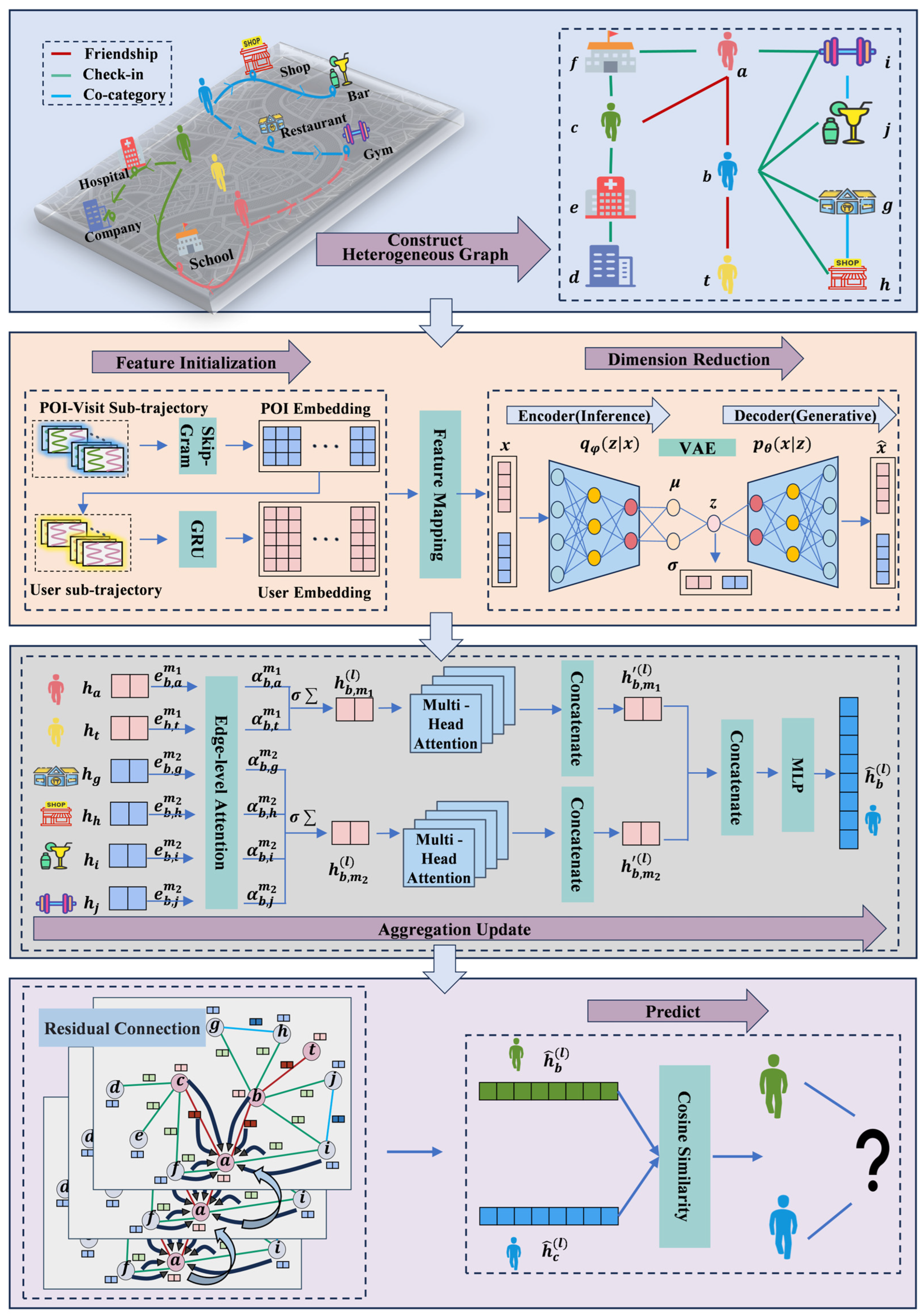
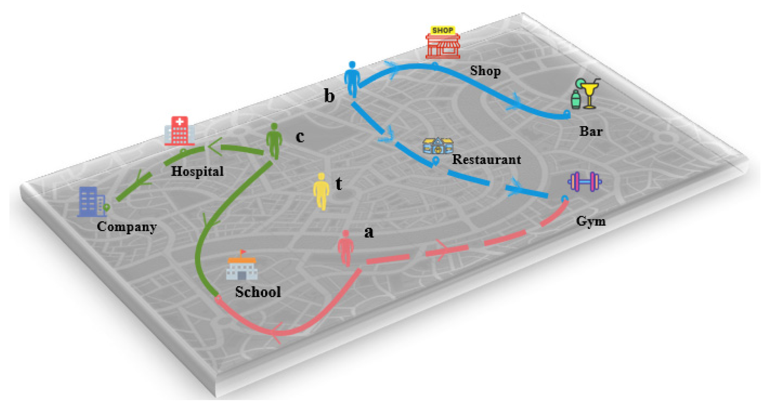
  • Heterogeneous Graph Construction: In response to the difficulty of processing rich heterogeneous data in LBSNs and the challenge that traditional graph models face in balancing complexity and information extraction, this paper proposes a heterogeneous graph model consisting of two types of nodes and three types of edges. This model can extract topological and semantic information from the network, enabling a better understanding and utilization of the complex structure in LBSNs.
  • Node Feature Embedding Learning Module: To address the difficulty of extracting precise and effective node features from the complex spatiotemporal data in Location-Based Social Networks (LBSNs), a strategy combining Skip-Gram and Lite-GRU is employed. Skip-Gram effectively captures the contextual relationships between POIs. In this paper, user trajectories are divided by day. Considering that sub-trajectory nodes are relatively few and contain dependencies, Lite-GRU, with its simplified gating mechanism, offers superior computational efficiency compared with LSTM and Transformer models. Unlike the bidirectional structure of BiLSTM, Lite-GRU uses unidirectional information flow, avoiding redundant information, and is more suited to the non-sequential nature of check-in behavior. While Transformer has advantages in modeling long sequences, its dense positional encoding mechanism can lead to overfitting under sparse data and cold start problems. In contrast, Lite-GRU handles temporal dependencies more effectively through a dynamic gating mechanism. Therefore, we use the Skip-Gram model to learn POI embeddings and combine it with Lite-GRU to learn user embeddings with temporal data processing capabilities, ultimately generating high-quality embedding vectors.
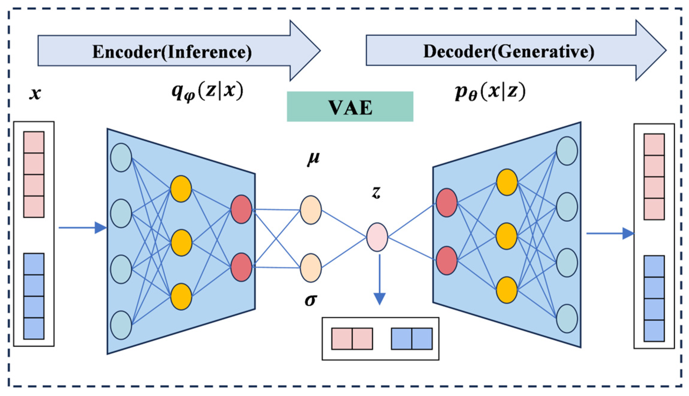
  • VAE Module: To tackle the high dimensionality and noise problems of LBSN data, this paper introduces VAE, which can extract useful features from high-dimensional noisy data, reduce dimensionality, and mitigate noise interference, thereby enhancing the model’s robustness. Considering that VAE can better capture complex nonlinear relationships while maintaining global topological structures, it overcomes the linear limitations of Principal Component Analysis (PCA), avoids the overfitting issues that may arise with AutoEncoder (AE), and is more efficient than t-Distributed Stochastic Neighbor Embedding (t-SNE) when handling large-scale datasets.
  • Edge-Level Attention: In response to the challenge of effectively parsing the complex network structure in LBSNs, where traditional methods fail to fully leverage edge properties and weights to accurately extract features and propagate information, this paper introduces an edge-level attention mechanism. By considering the properties and weights of edges, it learns the importance of different types of edges to enhance information propagation and feature extraction. Additionally, by combining node residual connections and multi-head attention, the node aggregation and propagation process is further optimized, effectively integrating the diverse information contained in different types of nodes and edges to obtain better node representations.
The rest of this paper is organized as follows: Section 2 introduces related work; Section 3 presents the research problem and relevant definitions; Section 4 provides a detailed description of the GEVEHGAN model; Section 5 designs experiments and analyzes the results; Section 6 concludes this paper’s findings.

2. Related Work

LBSNs combine geographical location information with social network functionality, allowing users to share location information and interact with others through mobile devices. The data on such platforms typically include user check-in records, review content, social relationships, and geographical location information, providing crucial support for various research and practical applications. The application scenarios of LBSNs are broad, covering areas such as POI recommendation [27,28,29], friend recommendation [30,31,32], spatiotemporal analysis [33,34], social interaction [35,36], and privacy protection [37,38,39]. In the context of friend recommendation, identifying potential friend relationships from massive data has become a critical issue that needs to be addressed. This section will explore the traditional methods and Graph Neural Network methods in detail.

2.1. Traditional Methods

Friend link prediction is a core problem in social network analysis, essentially predicting potential links by calculating the similarity between nodes. Traditional methods for friend link prediction mainly rely on the local topological structure of nodes. Common similarity measurement metrics include Jaccard [40], AA Adamic–Adar (AA) [41], Preferential Attachment (PA) [42], Resource Allocation (RA) [43], and the Salton index (SI) [44]. These methods evaluate similarity by analyzing the adjacency relationships of nodes. For example, CN assumes that two nodes with more common neighbors are more likely to be similar. Additionally, some path-based methods, such as Local Path (LP) [45], the Katz index [46], and Shortest Path (SP), consider path lengths and weights. For instance, the Katz index weights all paths and gives shorter paths higher importance, making the contribution of short path nodes to similarity more prominent.
In recent years, several methods have been proposed to improve the accuracy and efficiency of link prediction. Rafiee et al. [47] proposed the CNDP algorithm, which combines topological features such as the network’s average clustering coefficient and the number of shared neighbors, and calculates node similarity using an adaptive penalty method, enhancing prediction accuracy. Yuliansyah et al. [48] proposed the DGLP method inspired by Newton’s law of gravitation, which addresses the cold-start problem for new users joining the network, enhancing the model’s adaptability to new nodes. Aziz et al. [49] combined the Katz index and the AA index, using local path information and local information within a specified distance to further improve prediction accuracy. Ayoub et al. [50] introduced a non-parametric similarity measure combining local and global features to reduce the impact of high node degrees on prediction, effectively reducing biases when node degrees are large. In practice, these methods are often used in combination, with some studies combining local and global similarity metrics or introducing other network features (such as node degree centrality, closeness centrality, betweenness centrality) to enhance accuracy and robustness.
Although these traditional methods improve prediction performance to some extent, they mainly rely on the local topological structure. They also have clear limitations when dealing with the rich heterogeneous data and spatiotemporal characteristics in LBSNs. As the complexity of LBSN data increases, the effectiveness of traditional methods gradually diminishes, particularly when considering heterogeneous nodes and edges, where the prediction accuracy significantly declines. Therefore, how to incorporate geographic, social, and interest information from LBSNs into graph structures for friend link prediction has become a key problem in the current research.

2.2. Graph Neural Network Methods

With the development of deep learning technologies, Graph Neural Networks (GNNs) have become an important tool for solving social network link prediction problems. GNNs can effectively integrate node information and topological structure, providing strong support for modeling user behavior in LBSN data. Depending on the graph structure, GNN models can be divided into three categories: homogeneous graphs, heterogeneous graphs, and hypergraphs.

2.2.1. Homogeneous Graph Methods

Models like GCN [51] effectively capture the local structure and feature representations of nodes through semi-supervised learning, widely applied in link prediction within social networks. However, they incur significant computational overhead in large-scale graphs and fail to fully account for heterogeneous information. The Light Graph Convolutional Network (LightGCN) [52] simplifies the neighbor aggregation operation in the GCN model, improving training efficiency and reducing computational complexity, but it is less effective than more complex GNN models at capturing intricate interactions. GraphSAGE generates low-dimensional embedding representations to predict unobserved connections by sampling and aggregating neighborhood features, reducing computation in large-scale graphs but potentially overlooking some low-frequency and important adjacency information. The Multiscale Spatio Graph Convolution Network (MSGCN) [53] integrates multiple social relationships to generate personalized friend recommendations, capturing complex user behavior, but still suffers from data sparsity. The graph autoencoder proposed by Berg et al. [54] generates latent features via convolutional layers, suitable for structured data but less effective in large-scale graphs. Hamilton et al. [23] mitigated this issue by using neighborhood sampling methods. Velivckovic et al. introduced GAT, which weighs the importance of adjacent nodes using attention mechanisms, overcoming the limitations of the traditional GCN in aggregating neighbor information.

2.2.2. Heterogeneous Graph Methods

However, the inherent heterogeneity in real-world data presents new challenges, leading the current research focus to shift toward Heterogeneous Graph Neural Networks.
Heterogeneous Graph Neural Networks (HetGNNs) [55], metapath2vec [56], HAN [25], and Metapath Aggregated Graph Neural Networks (MAGNNs) [57] are typical methods from earlier studies. HetGNN strengthens node content representation through a combination of random walks and Bi-LSTM, especially encoding heterogeneous content such as text and images. However, it was not specifically designed to handle spatiotemporal trajectory information in LBSNs. HAN is the first hierarchical attention model that simultaneously considers both node-level and semantic-level importance. However, it only focuses on the two terminal nodes and ignores the information between them. MAGNN overcomes this limitation by aggregating information both within and between metapaths, effectively extracting structural and semantic information from different types of nodes and edges. However, MAGNN relies on manually designed metapaths to guide information propagation and lacks a dedicated mechanism to handle spatiotemporal information and dynamic changes. Thus, it is limited when dealing with user behaviors with spatiotemporal characteristics in LBSNs. The Heterogeneous Temporal Graph Neural Network (HTGNN) [58] focuses on capturing the dynamic changes of social relationships, suitable for modeling temporal information, but does not model the noise characteristics in LBSNs, which may limit its robustness when faced with noisy data. Some subsequent studies have also focused on processing heterogeneous graphs. HeteroGraphRec [59] uses graph convolution to analyze user interest similarities and considers multiple connection paths. The H2Re [60] model uses a random walk strategy to generate node sequences, combining homogeneous and heterogeneous information to improve recommendation accuracy, but the sparsity issue may affect convergence speed. and the model is highly sensitive to edge weights, which may ignore some important information.

2.2.3. Hypergraph Methods

In the hypergraph domain, methods like Hypergraph Convolutional Networks (HyperGCNs) [61], Hypergraph Networks with Hyperedge Neurons (HNHNs) [62], and Hypergraph Neural Networks (HGNNs) [63] rely on hypergraph Laplacian operators based on GCN. The HyperGCN method treats the learning problem as an approximation of graph learning by pairing the vertices connected by hyperedges to approximate the hyperedges in the hypergraph. Other hypergraph models, such as the Universal Graph Neural Network (UniGNN) [64], extend several GNN models to hypergraphs and propose a unified framework for explaining message-passing methods in Graph and Hypergraph Neural Networks. AllSet [65] is also the latest unified framework for Hypergraph Neural Networks, implementing Hypergraph Neural Network layers as a combination of two multi-set functions: AllDeepSets and AllSetTransformer. However, all of these hypergraph models ignore the heterogeneous semantic information in hypergraphs, which is one of the reasons for our research on GEVEHGAN.
Although existing Graph Neural Network methods have made progress in handling heterogeneous information in LBSNs, they still face challenges in integrating spatiotemporal trajectory information and addressing high-dimensional noise. Therefore, this paper combines the Lite-GRU module to learn user mobility trajectory information, effectively capturing the dynamic changes in check-in trajectories in LBSNs, making it particularly suitable for modeling spatiotemporal features. Additionally, the VAE module is introduced to leverage the dimensionality reduction capabilities of Variational Autoencoders, effectively reducing high-dimensional noise in LBSN data, thereby improving the usability and robustness of the data.

3. Problem and Definition

3.1. Problem Description

The aim of this study is to fully utilize user social relationships and historical check-in information to construct a heterogeneous graph G , and, based on this graph, learn a model: F u i , u j 0 ,   1 . The objective is to predict the probability F ( u i , u j ) that two users, u i and u j , will establish a friend link in the future. In this context, the heterogeneous graph G is defined as: G = V , E , R , C , a t t r v , a t t r e , where the components are as follows:
V : the set of nodes (users and POIs).
E : the set of edges (relationships between users or between users and POIs).
R : the set of node types (e.g., user nodes, POI nodes).
C : the set of edge types (e.g., social relationships, check-ins).
a t t r v : a function that defines the attributes of nodes.
a t t r e : a function that defines the attributes of edges.

3.2. Relevant Definitions

Definition 1.
User and POI: In LBSN data, the set  U = u 1 , u 2 , . . . , u m  represents  M  users, and the set   V = v 1 , v 2 , . . . , v n  represents  N  POIs. The information of each POI  v V  includes its geographical coordinates  l v  (latitude and longitude) and the category of the POI  c v , such as cinema, restaurant, etc.
Definition 2.
Friendship relationship  u i , u j  represents a friendship relationship between user  u i U  and user  u j U . If there is a friendship definition between them, it is labeled as  y i , j = 1 ; otherwise,  y i , j = 0 . The set  F u i = u 1 , u 2 , . . .  represents the friend list of user  u i , and  F U = F u 1 , F u 2 , . . . , F u m  represents the friend lists of all  M  users.
Definition 3.
Check-In Activity: For each user   u i U , each check-in record is denoted by  ( u i , v j , t k ) , indicating that user   u i  visited POI  v j  at time  t k . By combining the definition check-in record of user  u i  with the POI’s location and category, we obtain the check-in activity of user  u i , represented as 5-tuple  H u i t k = ( u i , v j , t k , l v j , c v j ) , where user  u i  visited POI  v j  at time  t k , and the location of POI  v j  is  l v j , with the category  c v j .
Definition 4.
User’s Historical Check-In Trajectory: All check-in activities of use  u i U  form their historical check-in trajectory  H u i = H t 1 u i , H t 2 u i , . . . , H t 3 u i . The set  H U = H u 1 , H u 2 , . . . , H u m  represents the historical check-in trajectories of all  M  users.
Definition 5.
Co-Category: if category  c i  of POI   v i V  is the same as category  c j  of POI   v j V , then there exists a co-category relationship between POI  v i  and POI  v j .

4. Methods

In this section, we provide a detailed introduction to the GEVEHGAN model, which is a Heterogeneous Graph Attention Network for friend link prediction. The model consists of five components: heterogeneous graph construction, node embedding learning based on Skip-Gram and Lite-GRU, VAE dimensionality reduction and denoising, feature aggregation and update based on edge-level attention, multi-head attention, and residual connections, and finally, friend link prediction. Figure 1 presents an overview of our framework. Although our model mainly focuses on capturing location check-ins and social relationships, there are some potential factors that have not been considered. The current model only captures directly connected social relationships, while ignoring multi-hop social influence and text-based interactions. Multi-hop social influence refers to the idea that users’ social relationships are not limited to directly connected friends but instead affect each other indirectly through multiple social links. This is particularly important in large-scale social networks, especially those with significant long-tail effects. Furthermore, text-based interactions (such as comments and likes between users) play a crucial role on many social platforms and may influence relationships between users. However, our current research mainly focuses on location check-ins and social relationships, without incorporating text-based interactions into the model. Future research could consider including these factors to further improve the model’s accuracy and generalization ability.

4.1. Constructing a Heterogeneous Graph

Although adding more types of nodes and edges can enhance the expressive power of a heterogeneous graph, an excessive number of node and edge types can significantly increase computational complexity and resource demands, potentially introducing information redundancy and noise, which could affect model performance. On the other hand, having too few types of nodes and edges may lead to insufficient information representation, making it difficult to capture the complex relationships between user behaviors and POIs, thereby reducing prediction accuracy. Therefore, when constructing the heterogeneous graph, it is necessary to strike a balance between maintaining the complexity of the graph and ensuring computational efficiency.
In this study, a user–POI heterogeneous graph is constructed based on users’ historical check-in records and social relationships in LBSN. This graph consists of user nodes, POI nodes, and three types of edges: friend edges, check-in edges, and co-class edges. The initial features of each type of relationship edge are as follows:
Friend edges: connect two users with a friendship relationship, and the feature of the edge is the distance between the approximate activity centers of these two users.
Check-in edges: connect a user to a POI they have visited, and the feature of the edge is the frequency of the user’s check-ins during different time periods, and the distance between the user and the POI.
Co-class edges: connect POIs with the same category, and the feature of the edge is whether the category labels of these two POIs are the same, along with the geographical distance between them.

4.2. Node Feature Learning

Node feature learning is a critical step in heterogeneous graph processing. Especially when dealing with large-scale and sparse POI data, choosing the appropriate embedding learning method is crucial. To capture the local relationships between nodes while balancing computational efficiency and sparsity issues, we use the Skip-Gram model to learn the embeddings for POI nodes. The Skip-Gram [66] model learns high-quality word vector representations by predicting context words, effectively capturing the spatial semantic relationships between different POIs. To improve training efficiency, hierarchical softmax and negative sampling techniques are used, significantly reducing computational complexity and speeding up the training process. In this way, Skip-Gram can efficiently train on large-scale datasets and learn high-quality vectors that represent the potential relationships between POIs.
For large-scale user behavior data, considering its sequential nature and long-term and short-term dependencies, we use the Lite-GRU model to learn the embeddings for user nodes, while making a trade-off between computational efficiency and robustness. Lite-GRU [67] is a lightweight recurrent neural network unit that merges gating mechanisms and uses the ReLU activation function, reducing the parameter count by over 30% while maintaining strong temporal modeling capabilities. This feature makes Lite-GRU particularly well suited for handling large-scale user trajectory data, offering significant advantages in applications that require efficient computation and real-time processing.

4.2.1. Learning POI Embeddings

In LBSN data, the historical check-in records H u i = H t 1 u i , H t 2 u i , . . . of each user u i U are represented as a user trajectory sequence T u i , where the user check-in trajectory is shown in Figure 2. To reduce computational complexity and capture richer semantic patterns of movement, we divide the original trajectory T u i of each user u i by day, thus obtaining a series of continuous sub-trajectories T u i = T 1 u i , T 2 u i , . . . .
Subsequently, we use a Skip-Gram-based model to learn the sub-trajectories of all users to obtain the embedding of POI v j V . The Skip-Gram model, commonly used for learning word embeddings, maps words to a low-dimensional vector space while preserving semantic relationships. In this paper, POIs are treated as “words”, and user sub-trajectories are treated as “sentences”. To incorporate more temporal information, the initial feature Ψ v j of POI v j not only includes spatial features like geographic location l v j and venue category c v j , but also considers the average visit frequency m of the location as a temporal feature. For a given POI v j V , we define its context as C ( v j ) , where C ( v j ) = { v j c , . . . , v j + c } , and c represents the sliding window size. The embedding of POI v j   Ψ v j is learned by maximizing the probability of predicting its context, i.e., the probability of the co-occurrence of context POIs with POI v j in the sub-trajectory T k u i containing v j , as shown in Equation (1):
max v l C ( v j ) exp ( Ψ v j T Ψ v l ) v = 1 | c | exp { Ψ v j T Ψ v }
For each POI v j , the final embedding vector Ψ v j f i n a l of POI v j is obtained by averaging the learned embedding vectors Ψ v j across all sub-trajectories containing v j .

4.2.2. User Embedding Learning

After learning the embeddings of all POIs, the user sub-trajectory T k u i T u i is fed into the Lite-GRU-based model, where the sub-trajectory T k u i contains T k time steps, and x k , t represents the feature input at time step t for sub-trajectory T k u i , i.e., the embedding of POI v , Ψ v f i n a l R d , where R represents the set of real numbers.
First, the hidden state h k , 0 R d is initialized, and, then, at each time step t , the reset gate r k , t is computed as shown in Equation (2), the update gate z k , t is calculated as shown in Equation (3), the candidate hidden state h ~ k , t is calculated as shown in Equation (4), and the hidden state h k , t is updated as shown in Equation (5).
To reduce computational redundancy and decrease the model storage requirements, we merge the reset gate and update gate into a single common gate by sharing the weight matrices. The computation method is shown in Equation (2):
z k , t = σ ( W · [ h k , t 1 , x k , t ] + b )
To avoid the gradient vanishing problem of tanh, we use the ReLU activation function to compute the hidden state, which effectively improves the training performance of deep networks. The final hidden state h k , t is calculated as shown in Equation (3):
h k , t = ( 1 z k , t ) h k , t 1 + z k , t R e L U ( W h · [ z k , t h k , t 1 , x k , t ] + b h )
where W R d × d , W h   R d × d represent the shared weight matrix and the candidate hidden state weight matrix, respectively, and b R d ,   b h R d represent the biases for the merged gate and candidate hidden state, respectively. σ · is the nonlinear activation function of the neuron, the sigmoid function, whose calculation method is shown in Equation (4):
f ( x ) = 1 1 + e x
Finally, the embedding of sub-trajectory T k u i is represented by the hidden state at the last time step h k , T k , and the embedding of user u i , E u i , is obtained by averaging the embeddings of all sub-trajectories of user u i , as shown in Equation (5):
E u i = 1 N N k = 1 h k
where E u i is the embedding of user u i , N is the total number of sub-trajectories for user u i , and h k is the final hidden state of the k -th sub-trajectory of user u i .

4.2.3. Feature Mapping

Since the user nodes, POI nodes, and various relationship edges in the heterogeneous graph have different semantics and feature spaces, their sizes, ranges, and distributions are typically not uniform. Therefore, after feature initialization, we map the features of the nodes and edges so that they are represented in the same dimension and feature space. The feature mapping calculations for nodes and edges are shown in Equations (6) and (7):
h v = W r v · X v
where h v R d n o t e represents the mapped feature of node v V , X v R d r v is the original feature of node v , r v R is the node type of v , and W r v R d n o d e × d r v is the mapping matrix specific to node type r v .
h e = W c e · X e
where h e R d e d g e represents the mapped feature of edge e ε , X e R d c e is the original feature of edge e , c e C is the edge type of e , and W c e R d n o d e × d c e is the mapping matrix specific to edge type c e .

4.3. VAE Dimensionality Reduction and Denoising

In LBSNs, node features are typically high-dimensional and susceptible to noise interference due to factors such as the randomness of user behavior, measurement errors in location data, or inaccuracies during the network propagation process. Even after feature initialization, the node features may still contain a significant amount of noise, which can affect model performance. To address this issue, Variational Autoencoders as a generative model, can effectively perform dimensionality reduction while denoising. The architecture is illustrated in Figure 3.
The basic framework of VAE consists of three parts: encoder, latent variables, and decoder. First, the encoder network q z | x maps the input data x to the latent space z . Then, the decoder p x | z generates reconstructed data x ^ based on the latent variable z . The entire process can be achieved by optimizing the variational lower bound. Through this approach, VAE retains the main features of the data while removing noise during dimensionality reduction.

4.3.1. Encoder and Latent Space

The encoder is a neural network that maps the input data x to the latent space z . VAE assumes that the latent representation of the input data follows a Gaussian distribution and models the latent structure of the data through this distribution. Specifically, the encoder outputs the mean μ ( x ) and standard deviation σ ( x ) of the latent variable z , as shown in Equation (8):
q ( z | x ) = N ( z ; μ ( x ) , σ 2 ( x ) )
To sample from this distribution, VAE introduces the reparameterization trick, generating the latent variable z using Equation (9):
z = μ ( x ) + σ ( x ) ε , ε ~ N ( 0 , I )
where ε is noise sampled from a standard normal distribution, and μ ( x ) and σ ( x ) are the mean and standard deviation output by the encoder network. The symbol “⊙” represents element-wise multiplication.

4.3.2. Decoder and Data Reconstruction

The decoder is a neural network that maps the latent variable z back to the input space, generating reconstructed data x ^ based on the latent variable z . The output of the decoder is the conditional probability of the data, typically assumed to follow a Gaussian distribution, as shown in Equation (10):
p ( x | z ) = N ( x ; x ^ , I σ 2 )
where x ^ is the reconstructed data generated by the decoder based on the latent variable z , N represents a Gaussian distribution, σ 2 is the predefined reconstruction variance hyperparameter (which controls the denoising strength), and I denotes the identity matrix.

4.3.3. Variational Lower Bound

VAE is trained by maximizing the log-likelihood log p ( x ) of the data. However, directly computing p x is infeasible, Therefore, VAE uses variational inference by maximizing the variational lower bound (ELBO) to accurately reconstruct user behavior data and capture the interactions between users and locations, while ensuring that the latent space structure is reasonable, thereby learning the latent interests and behavior patterns of users.
The ELBO is calculated as shown in Equation (11):
L ( θ , ϕ ; x ) = E q ( z | x ) [ log p ( x | z ) ] D K L ( q ( z | x ) | | p ( z ) )
where θ and ϕ represent the neural network parameters of the decoder and encoder networks, respectively.
q z | x is the approximate posterior distribution of the latent variable zzz output by the encoder network, typically a Gaussian distribution;
p x | z is the conditional probability of the reconstructed data generated by the decoder;
D K L ( q ( z | x ) | | p ( z ) ) is the KL divergence, measuring the difference between the approximate posterior distribution q z | x and the prior distribution p z .
By maximizing the variational lower bound, VAE can optimize the representation in the latent space while maintaining the essential information of the data, thereby achieving dimensionality reduction.

4.4. Node Aggregation and Update

In heterogeneous graphs, the importance of a target node can be influenced by the types of edges and neighboring nodes, as different types of nodes and edges carry different semantic information.
To efficiently aggregate information from various types of nodes and edges in a heterogeneous graph, a more refined aggregation strategy is required. Specifically, we concatenate the target node features, neighbor node features, and edge features to create a joint input, ensuring the completeness of the information. Then, we apply a multi-head attention mechanism for parallel computation, and the outputs of each head are concatenated and passed through a multi-layer perceptron for nonlinear transformation. Finally, through cross-edge-type concatenation and residual connections, we achieve multi-level feature fusion, effectively enhancing the model’s nonlinear interaction ability, preserving the integrity of heterogeneous information, and optimizing the information aggregation process, thereby improving the model’s expressive power.

4.4.1. Edge-Level Attention

Assume that the target node i V and the neighboring node j V are connected by an edge e i j m 1 , where m 1 denotes the edge type. We compute the edge-type attention weight α i , j m 1 to measure the importance of node j to target node i through the edge e i j m 1 . The edge-type attention is based on improvements made in GAT and GATv2 [68]. While GAT performs excellently on homogeneous graphs, it cannot be directly applied to heterogeneous graphs because it ignores the types of nodes and edges. GATv2 improves upon this by optimizing the attention mechanism and adjusting the order of calculating attention coefficients, with scalar mappings placed last, thereby enabling dynamic attention and enhancing expressive capacity. In this paper, by extending the original graph attention mechanism and integrating improvements from GATv2, we introduce edge-type attention to more finely aggregate information in heterogeneous graphs. Specifically, edge-type information is incorporated into the attention calculation. The calculation is given by the following Equation (12):
α i , j m 1 = exp ( a T L e a k y Re L U ( W h [ h i | | h j | | h e i j m 1 ] ) ) n N i m 1 exp ( a T L e a k y Re L U ( W h [ h i | | h n | | h e i n m 1 ] ) )
The edge-level attention mechanism designs independent learnable parameters for each edge type, splicing the features of the target node, neighbor node, and edge, calculating the original score after linear transformation and LeakyReLU activation, and finally normalizing by softmax to obtain the attention weight α, which is different from the standard GAT only considering the node features. It explicitly models the edge-type features (such as social relationship strength, spatiotemporal information, etc.). The model can distinguish the different functions of user–user edge (focusing on interest influence) and user–place edge (focusing on behavior preference), and capture the social relationship between users and the diversified interaction between users and places more accurately.
Here, α i , j m 1 represents the attention weight between node i and node j connected by the edge of type m 1 , n N i m 1 denotes the set of neighboring nodes connected to target node iii via edges of type m 1 , h i , h j , h n R d n o d e represent the feature vectors of nodes i , j , n , respectively, h e i j m 1 R d e d g e represents the feature vector of the edge e i j m 1 , and h e i n m 1 represents the feature vector of the edge e i n m 1 connecting target node i and node n , with edge type m 1 . α T R d is the learnable edge-type attention vector, and W h R d × 2 d n o d e + d e d g e is the learnable edge-level attention weight matrix. The symbol | | indicates concatenation, and L e a k y R e L U · is the activation function.

4.4.2. Residual Connections

To capture the complex interactions in the user–POI heterogeneous graph and enhance the model’s expressive power, this paper adopts a multi-layer propagation structure to explore higher-order information. However, in GNNs, stacking multiple propagation layers may lead to issues such as gradient vanishing or over-smoothing, which can affect the model’s training performance. To address this problem, this paper introduces node pre-activation residual connections [69,70,71] to alleviate the negative effects of deep networks.
Residual connections help preserve the uniqueness of node representations and prevent feature loss and reduced distinguishability between nodes caused by deep propagation. By adding residual connections at each propagation layer, the model can effectively avoid over-smoothing of information, making node features easier to learn. The update of node representations by edge type m 1 is shown in the following equation:
h i , m 1 ( l ) = σ ( n N i m 1 α i , n m 1 ( l ) W ( l ) [ h n ( l 1 ) | | h e i n m 1 ( l 1 ) ] + W r e s ( l ) h i , m 1 ( l 1 ) )
User behavior data and the interactions between users and locations often involve multi-level complex dependencies. Residual connections help preserve key information in user behavior and interaction data, allowing the model to retain important details while facilitating deeper learning without the risk of losing critical information during the aggregation process.
Here, l denotes the l -th layer, h i , m 1 ( l ) represents the target node i ’s representation connected by edge type m 1 in the current layer, σ · is the activation function, W l represents the learnable weight matrix for aggregating the neighboring node representations and edge representations at the current layer, and W r e s ( l ) R d l + 1 × d l is the learnable residual connection transformation matrix, which maps the node representation from the previous layer to the current layer’s dimension when there is a dimensionality change.

4.4.3. Multi-Head Attention

Multi-head attention enables the model to obtain richer graph information by computing attention weights from different heads in parallel, thereby enhancing its expressive power. The target node i is connected to its neighboring node set N i m 1 via edge type m 1 , and the multi-head attention mechanism is used to aggregate the information from these neighboring nodes. Specifically, the representation of the target node i is updated by each attention head. The computation is given by Equations (14) and (15):
h ^ i , m 1 , k ( l ) = n N i m 1 α i , n , k ( l ) W k ( l ) [ h n ( l 1 ) | | h e i n m 1 ( l 1 ) ]
h i , m 1 ( l ) = σ ( | | k = 1 K h ^ i , m 1 , k l + W r e s ( k ) ( l ) h i , m 1 ( l 1 ) )
where h ^ i , m 1 , k ( l ) represents the aggregated feature of the k -th head through the m 1 -type edge at the l -th layer for the neighboring node set, K denotes the number of attention heads, and k represents the k -th attention head. h ^ i , m 1 ( l ) is the representation of target node i through the m 1 -type edge at the l -th layer.
Finally, to integrate the results from the multi-head attention mechanism, the outputs corresponding to different edge types are concatenated using the concatenation operation and mapped nonlinearly through a Multi-Layer Perceptron (MLP) to obtain the final node representation h ^ i l . The computation is given by Equations (16) and (17):
h ^ i l = | | z = 1 Z h i , m z ( l )
h ^ i l = M L P ( h ^ i l ) = R e L U ( W 2 R e L U ( W 1 h ^ i l + b 1 ) + b 2 )
Each head in the multi-head attention mechanism focuses on different aspects of the edge type. For example, at the check-in edges, one head might focus more on the type of location (e.g., restaurant, tourist spot), while another head might focus on the frequency of user behavior at these locations. By using the multi-head attention mechanism, the model can learn different influencing factors in parallel for different types of edges, enabling it to more accurately understand the multiple factors influencing user behavior. This improves the model’s predictive accuracy regarding user interests and behavior.
Where | | represents the concatenation operation, Z is the number of edge types, W 1 , W 2 are the weight matrices, b 1 , b 2 are the biases, and ReLU is the activation function.

4.5. Link Prediction

We use cosine similarity to measure the similarity between users and design a new joint loss function to ensure that the model learns effective user representations.

4.5.1. Cosine Similarity

After obtaining the final node representations for user node i and user node j , cosine similarity is used to evaluate the potential friendship link between users i and j , denoted as s ( i , j ) . The computation is shown in Equation (18):
s ( i , j ) = h ^ i L h ^ j L | | h ^ i L | | | | h ^ j L | |
where h ^ i L and h ^ j L represent the final node representations of user i and user j , respectively, and · denotes the vector norm.

4.5.2. Joint Loss Function

The computations are shown in Equations (19)–(22):
L B C E = 1 N ( i , j ) ( E N ) [ y i j l o g ( s ( i , j ) ) + ( 1 s ( i , j ) ) l o g ( 1 s ( i , j ) ) ]
L R E C = 1 N i = 1 N ( x i x ^ i ) 2
L K L = 1 2 i ( 1 + log ( σ i 2 ) μ i 2 σ i 2 )
L t o t a l = λ 1 L B C E + λ 2 L R E C + λ 1 L K L
where y i , j 0,1 represents the true positive or negative label for the pair of users u i and u j , and the datasets for positive and negative samples are denoted as P (positive sample dataset) and N (negative sample dataset). N represents the sample size, L B C E represents the cross-entropy loss, L R E C represents the reconstruction loss, and L K L represents the KL divergence loss. λ 1 , λ 2 , and λ 3 represent their respective weights.

5. Experimental Setup

5.1. Dataset

In this paper, we select the check-in data from six cities—New York (NY), Tokyo (TKY), São Paulo (SP), Jakarta (JK), Istanbul (IST), and Kuala Lumpur (KL)—from the Foursquare dataset, based on a comprehensive consideration of geographic coverage, cultural diversity, data completeness, and city size. These cities represent different geographic regions (North America, Asia, South America, Europe, and Southeast Asia), encompass diverse cultural backgrounds (Western, East Asian, and Islamic), and provide complete user check-in and social relationship data. This enables the dataset to adequately reflect the diversity of user behavior and social relationships in LBSNs. To ensure a balanced ratio of positive and negative samples, negative samples are randomly selected from pairs of users without friendship relationships within the LBSN.
In the data preprocessing stage, UTC time is first converted to Unix timestamps and parsed into structured time information to normalize the raw check-in records, supporting subsequent time modeling. Next, POI data are enhanced through standardizing identifiers, adding semantic information, and other processing. The total number of check-ins for each POI and user in the dataset is calculated, and, based on prior research [29,72], low-frequency POIs with fewer than 10 check-ins are removed to suppress noise and enhance the model’s ability to capture stable user patterns. At the same time, users with fewer than or equal to 2 check-ins are filtered out to ensure the data effectively reflect social behavior patterns. Finally, based on the cleaned data, three types of heterogeneous edge relations are constructed: user–POI check-in relations, user–user friendship relations, and POI–POI co-category relations. Different edge features (such as visit frequency, geographic distance, category labels, etc.) are defined to comprehensively quantify user preferences, social relationships, and potential associations between POIs, providing high-quality input for subsequent heterogeneous graph modeling. The data are then randomly split into training, validation, and test sets at a 7:2:1 ratio. The details of the preprocessed data are shown in Table 1.

5.2. Evaluation Metrics

To ensure the results are reasonable and fair, we adopt three widely used evaluation metrics for the friend link prediction task. These include the Area Under the ROC Curve (AUC), Average Precision (AP), and Top@K accuracy to evaluate model performance. The formulas for these metrics are provided in Equations (23)–(25).
A U C = i M + N ( s p > s n ) + 0.5 i M + N ( s p s n ) M N
M and N represent the number of positive and negative samples, respectively, and s p and s n represent the scores for positive and negative samples, respectively. ( s p > s n ) and ( s p s n ) represent a pair of positive and negative samples where the positive sample’s score is greater than or less than or equal to the negative sample’s score.
A P = 1 N k = 1 N ( P ( k ) r e l ( k ) )
N represents the total number of recommended results, P k is the precision at the top k recommendations, and r e l k is the relevance of the k -th recommendation. If relevant, r e l k = 1 , otherwise r e l k = 0 .
T o p @ K = m K
K represents the total number of the top K recommendations, and m represents the number of correctly recommended results among the top K recommendations.

5.3. Parameter Settings

The model training is conducted using PyTorch1.12. The experimental environment configuration of the model is shown in Table 2. The main parameters involved in the GEVEHGAN model during the experiment are shown in Table 3.

5.4. Baseline Methods

To comprehensively evaluate the performance of the GEVEHGAN model, we compare it with two categories of different methods.

5.4.1. Experimental Methods for Homogeneous Graphs

GCN: Utilizes Graph Convolutional Networks to learn node representations, assisting in node classification and prediction through information propagation. It captures node similarity and structural information.
GAT: Introduces an attention mechanism to automatically learn importance weights between nodes and update node representations. It can specifically learn the strength of node relationships in friend link prediction, improving accuracy.
GraphSAGE: Learns node representations by sampling and aggregating neighbor node features. It is efficient for training on large-scale homogeneous graphs and is suitable for friend link prediction using local neighbor information.

5.4.2. Experimental Methods for Heterogeneous Graphs

Metapath2vec: Leverages metapaths to learn node representations and performs random walks on heterogeneous graphs using the word2vec model. In friend link prediction, it can uncover potential relationships between different types of nodes, but its adaptability to complex social network structures is limited.
Heter-GCN: Used for processing heterogeneous graphs containing multiple types of nodes and edges. In friend link prediction, it can fully utilize the rich information in heterogeneous graphs.
MAGNN: Learns multi-layer node representations via meta-graphs to enhance expressiveness. In friend link prediction, it can capture complex social relationships by constructing different meta-graph structures.
AllSetTransformer [65]: this is the latest general hypergraph framework proposed by AllSet, with an attention-based set Transformer layer.
By comparing with these methods, the performance of the GEVEHGAN model can be more comprehensively evaluated, providing insights into its strengths and weaknesses in handling graph-structured data.

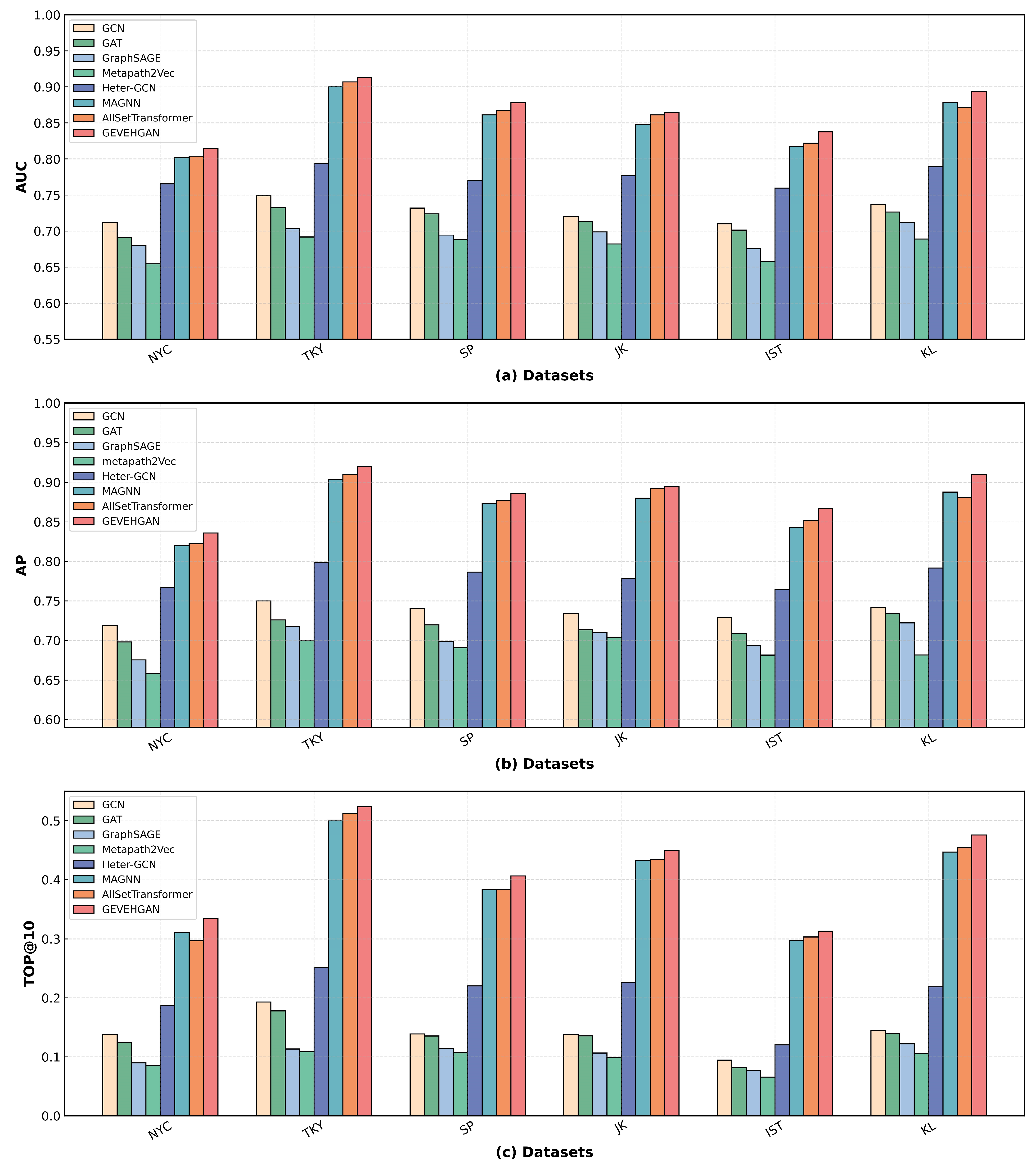
5.5. Comparative Experiments

We compare the GEVEHGAN model with six baseline methods, conducting ten repeated experiments for each model. The average values of AUC, AP, and Top@10 results from five repeated experiments are used as the final results. The experimental results are shown in Figure 4.
In the comparative experiments, we evaluate the performance of the GEVEHGAN model against seven other baseline models on six datasets. The results show that the GEVEHGAN model outperforms all other baseline models. Specifically, compared with the best performance of the baseline models, the GEVEHGAN model shows an average improvement of 1.52%, 1.61%, and 2.18% in AUC, AP, and Top@K, respectively. Notably, the performance improvements in the IST and KL datasets are significant. This is likely due to the rich information available in these datasets, such as user, POI, and friend numbers, which provide sufficient resources for the GEVEHGAN model to effectively mine topological and semantic information.
Among the seven models, Metapath2vec shows a relatively average performance. As an unsupervised learning method that mines heterogeneous graphs through random walks and learns node relationships using the heterogeneous Skip-Gram model, Metapath2vec fails to adequately consider the differences in node types and relationship types. It also does not fully exploit edge features, spatiotemporal information, or semantic information in the heterogeneous graph, limiting its performance in the friend link prediction task.
GraphSAGE performs similarly to Metapath2vec. Although GraphSAGE is a homogenous graph model, it aggregates neighbor information and stacks multiple layers to obtain higher-level node representations. Thus, it somewhat competes with Metapath2vec’s heterogeneous graph approach. However, the neighbor node sampling strategy of GraphSAGE reduces computational complexity but also limits its ability to fully leverage neighbor information.
GCN and GAT show similar performance and outperform GraphSAGE, which is also a homogenous graph method. This may be because GCN and GAT are more refined in capturing relationships between nodes, allowing them to more effectively utilize information from the graph structure. In contrast, GraphSAGE’s sampling strategy may lead to the loss of information.
Heter-GCN shows a significant improvement over both homogenous graph methods and Metapath2vec, demonstrating the importance of heterogeneous information in friend link prediction tasks. MAGNN AllSetTransformer performs even better than Heter-GCN. This may be because Heter-GCN fails to fully consider the rich spatiotemporal and semantic information in the LBSN data when constructing the heterogeneous graph. MAGNN, by incorporating metapaths and attention mechanisms, is able to capture higher-order interactions between nodes and better understand the importance of different nodes and metapaths, The higher-order set relationship modeling of hypergraphs connects multiple nodes through hyperedges, supporting cross-type and cross-hierarchy interaction propagation, further enhancing its performance in friend link prediction.
In the comparison between the GEVEHGAN model and the other seven models, an in-depth qualitative analysis is conducted across multiple dimensions, including graph model construction, node embedding, and dimensionality reduction denoising, along with information aggregation and propagation.
From the perspective of heterogeneous graph creation, GEVEHGAN combines two types of nodes—users and POIs—within the heterogeneous graph and explicitly models the multi-dimensional interactions of social, spatiotemporal, and semantic aspects through three relationships: friend edges, check-in edges, and co-occurrence edges. Unlike traditional homogeneous graph models (such as GCN, GAT, and GraphSAGE), GEVEHGAN provides a more comprehensive reflection of user behavior characteristics through multi-type edge fusion. Compared with Metapath2vec, Heter-GCN, and MAGNN, GEVEHGAN avoids the loss of semantic information and simplifies the model by directly modeling edge attributes (such as time and geographical distance). When compared with AllSetTransformer, GEVEHGAN is more precise in handling fine-grained user–POI interactions in LBSNs and can accurately distinguish edge semantics.
From the perspective of node embedding and dimensionality reduction denoising, GEVEHGAN significantly improves node embedding quality through multimodal embedding joint modeling and generative denoising. Compared with traditional models that rely on neighborhood aggregation (such as GCN, GAT, and GraphSAGE), GEVEHGAN reduces noise and captures the temporal dependencies in POI co-occurrence semantics and user trajectories. Through probabilistic compression of high-dimensional embeddings using VAE, GEVEHGAN effectively filters random check-in noise. Compared with Metapath2vec and Heter-GCN, GEVEHGAN’s Lite-GRU can capture short-term behavior sequences and enhance robustness through VAE, mitigating interference from sparse data. In comparison with MAGNN and AllSetTransformer, GEVEHGAN balances spatiotemporal continuity and semantic correlation, better adapting to the dynamic nature of user behavior in LBSNs, providing high-discriminatory low-noise embeddings for downstream tasks.
From the perspective of information aggregation and propagation, GEVEHGAN significantly enhances information aggregation and propagation through its edge-level attention mechanism and residual-enhanced heterogeneous information fusion architecture. Compared with traditional homogeneous models (such as GCN, GAT, and GraphSAGE), GEVEHGAN avoids edge-type semantic confusion caused by node-level attention and uniform aggregation, preserving key spatiotemporal behavioral information. It dynamically computes the weights of the three types of edges and combines multi-head attention with residual connections, improving edge semantic modeling accuracy. Compared with static heterogeneous models (such as Metapath2vec and Heter-GCN), GEVEHGAN flexibly handles the diversity of user–POI interactions in LBSNs and captures complex behavior patterns. Compared with more complex heterogeneous frameworks (such as MAGNN and AllSetTransformer), GEVEHGAN avoids noise introduction and over-smoothing issues by dynamically adjusting the intensity of information propagation and using residual connections. The precise-edge semantic modeling and multi-dimensional attention capture the synergistic influence of spatiotemporal, social, and interest factors, satisfying the heterogeneity and dynamics requirements of LBSN data.
Overall, heterogeneous graph methods are better at mining and utilizing the richer semantic and topological information in heterogeneous social networks, compared with homogenous graph methods that rely solely on topological information in social networks. The GEVEHGAN model proposed in this chapter, compared with previous heterogeneous graph methods, does not require manually designed metapaths but learns node representations directly from the entire heterogeneous graph. It not only considers the high-dimensional noise in LBSN data and the temporal features of user mobility trajectories but also takes into account the importance of different types of nodes and edges. These features enable the GEVEHGAN model to achieve better results in friend link prediction tasks.

5.6. Ablation Study

To evaluate the effectiveness of each module in the GEVEHGAN model, we conduct an ablation study using two representative datasets: NYC and TKY. A series of experiments are designed to evaluate the impact of the node feature learning module, VAE module, the edge-type attention mechanism, and the node residual connection mechanism. The specific experimental setups are as follows:
  • GEVEHGAN-Init: The node feature initialization module in the input layer is removed, and the heterogeneous graph node features are randomly initialized with small values. Other parts of the model remain unchanged.
  • GEVEHGAN-Vae: The Variational Autoencoder module is removed, and the initialized features are directly used. Other parts of the model remain unchanged.
  • GEVEHGAN-Att: The edge-type attention mechanism in the node feature learning process is removed, and the importance of neighbor nodes remains the same. Other parts of the model remain unchanged.
  • GEVEHGAN-Res: The node pre-activation residual connection mechanism is removed, and the traditional GNN node aggregation update method is used. Other parts of the model remain unchanged.
The results of the ablation study are shown in Figure 5. The experiments analyze the impact of each component on model performance, as detailed below:
  • Node Feature Embedding Module: After removing the node feature embedding module, the node’s initial features loses the semantic associations and temporal patterns obtained through pretraining, resulting in a reduction in the information available to the model when understanding user behavior and interests. The three metrics of the GEVEHGAN-Init model decrease by 4.11%, 4.51%, and 3.81%, respectively. This indicates that the features learned through Skip-Gram and Lite-GRU as the initial node features for the heterogeneous graph provide richer information for the nodes, significantly enhancing the model’s performance.
  • Variational Autoencoder Module: After removing the VAE module, the model fails to perform noise reduction on high-dimensional sparse features, leading to more irrelevant data being included in the information, thus reducing the clarity and usability of the features. The three metrics of the GEVEHGAN-Vae model decrease by 2.17%, 2.47%, and 2.42%, respectively. This shows that the VAE module condenses the key information from the original node features, removes redundancy and noise, and provides the model with more refined feature representations.
  • Edge-Type Attention Mechanism: After removing the edge-type attention mechanism, the model is unable to dynamically adjust the weights of the edges, resulting in an imbalance in the propagation of information across multiple relations, with key information not receiving enough attention. The three metrics of the GEVEHGAN-Att model decrease by 5.45%, 5.76%, and 4.42%, respectively. This demonstrates that the edge-type attention mechanism helps focus on key edge information, integrates multiple relationships to enhance feature representation, and improves information utilization efficiency through adaptive information selection and optimized propagation paths.
  • Node Residual Connection Mechanism: After removing the node residual connection mechanism, the information gradually diminishes during propagation through the deeper layers of the network, causing the model to lose the ability to maintain differentiation between nodes, leading to gradient vanishing and learning difficulties during training. The three metrics of the GEVEHGAN-Res model decrease by 3.06%, 3.87%, and 3.51%, respectively. This suggests that the node residual connection mitigates gradient issues, improves backpropagation, facilitates parameter updates, and prevents information loss. Additionally, it further improves feature fusion, leading to better representations and enhanced model performance.
Ablation experiments show that the four core components of GEVEHGAN make significant contributions to performance. These components ensure information quality through different mechanisms, e.g., feature initialization provides semantic priors, VAE performs noise filtering and dimensionality reduction, edge attention enables differentiated information propagation, and residual connections ensure effective training of deep networks. Overall, the collaborative effect of these components significantly improves the accuracy and robustness of the model in social relationship prediction tasks.

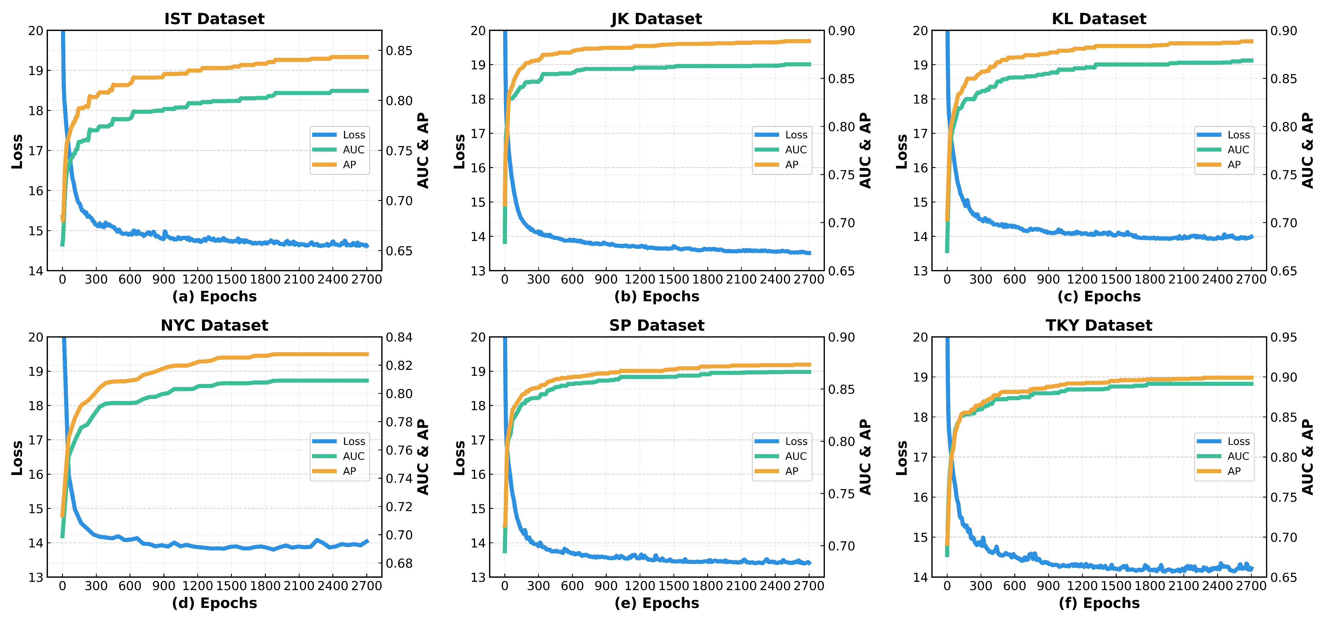
5.7. Model Performance Evaluation Experiment

We design model performance evaluation experiments on six datasets, monitoring the changes in metrics such as AUC, AP, loss, and Top@K across training epochs, in order to analyze the model’s performance optimization process.
As shown in Figure 6, both AUC and AP increase with the number of epochs. The rise in AUC reflects the improved ability of the model to distinguish between positive and negative samples, while the increase in AP indicates improved accuracy in predicting positive samples. Both metrics demonstrate improvements in the model’s learning and prediction accuracy. At the same time, loss decreases with epochs, meaning the deviation between model predictions and true labels reduces, indicating better fitting of the model.
As shown in Figure 7, Top@1 to Top@20 increase horizontally with the increase in epoch, indicating that the model’s prediction accuracy for each predefined ranking position continues to improve, allowing for more precise determination of the results at the corresponding ranks. At the same time, its vertical increase with epoch reflects that the model’s overall prediction capability across the entire ranking range has been comprehensively enhanced, with the result quality at all ranking positions being optimized.

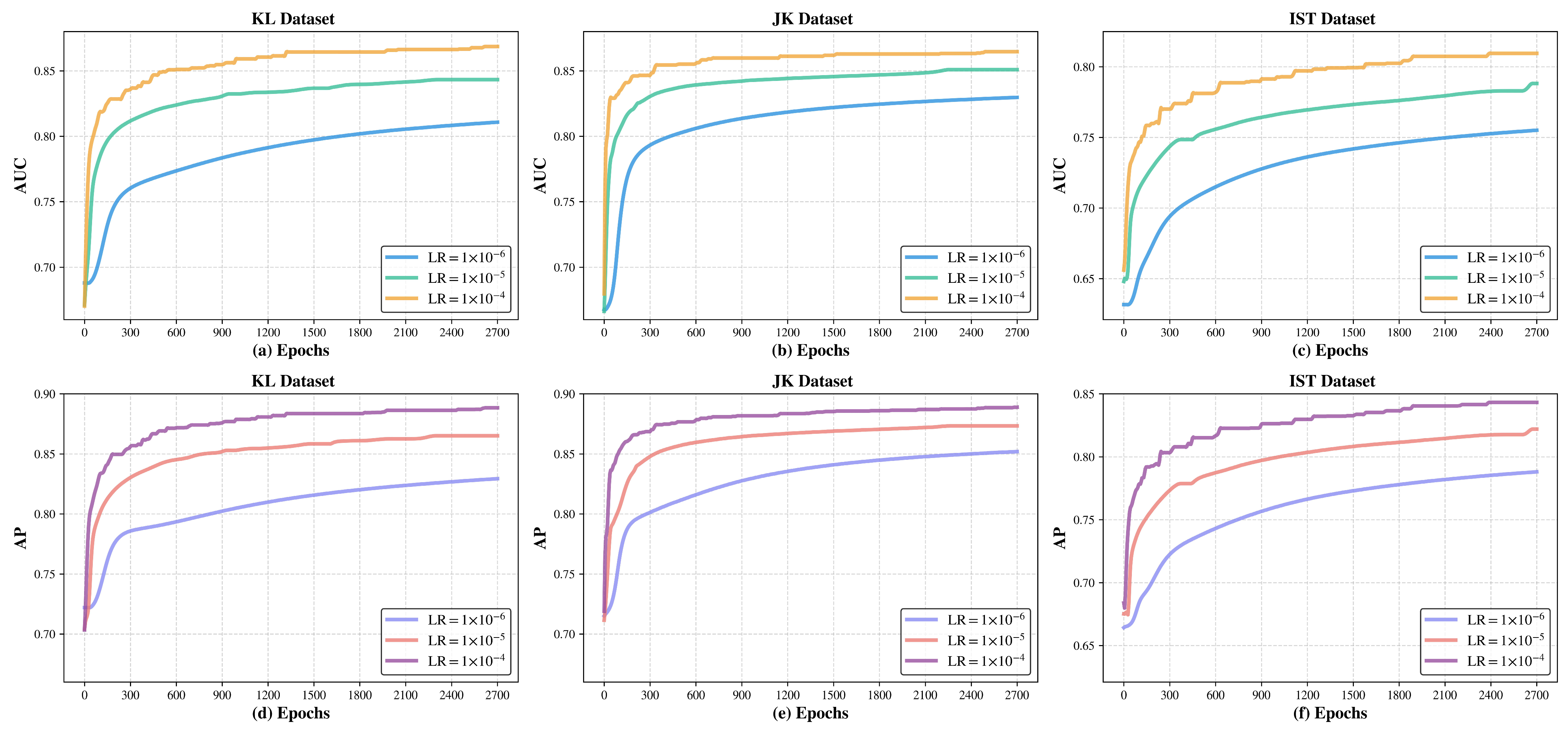
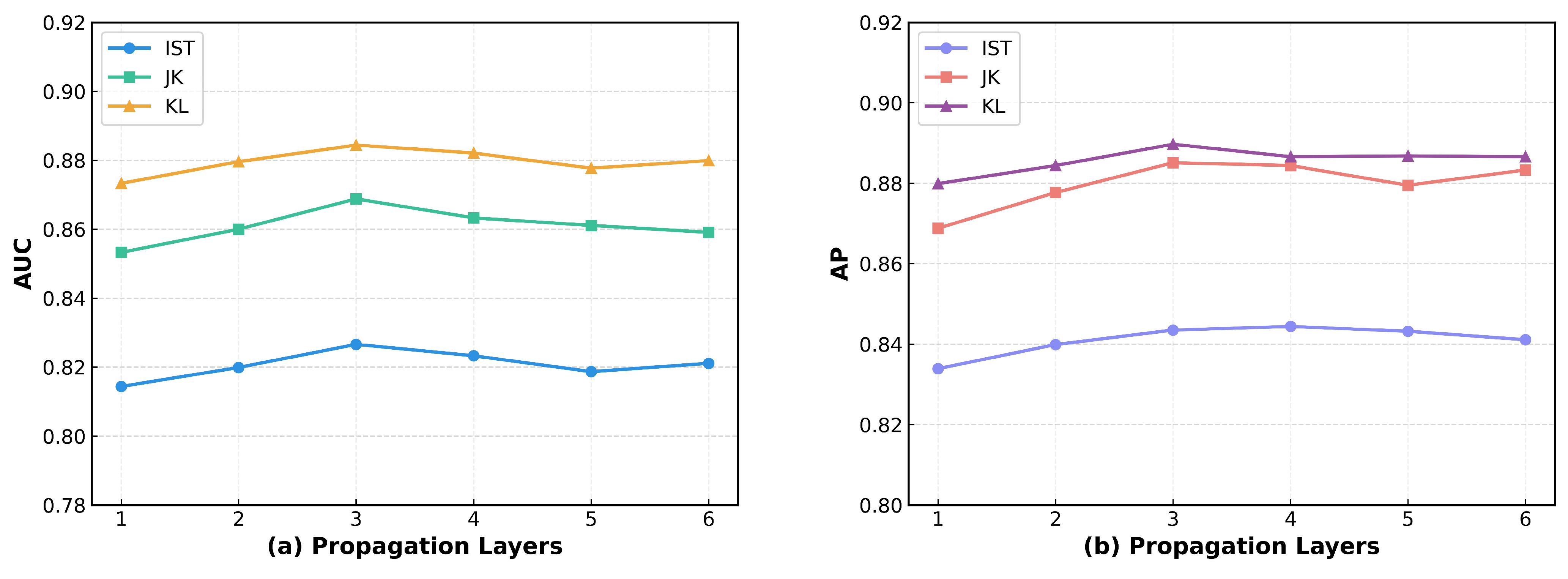
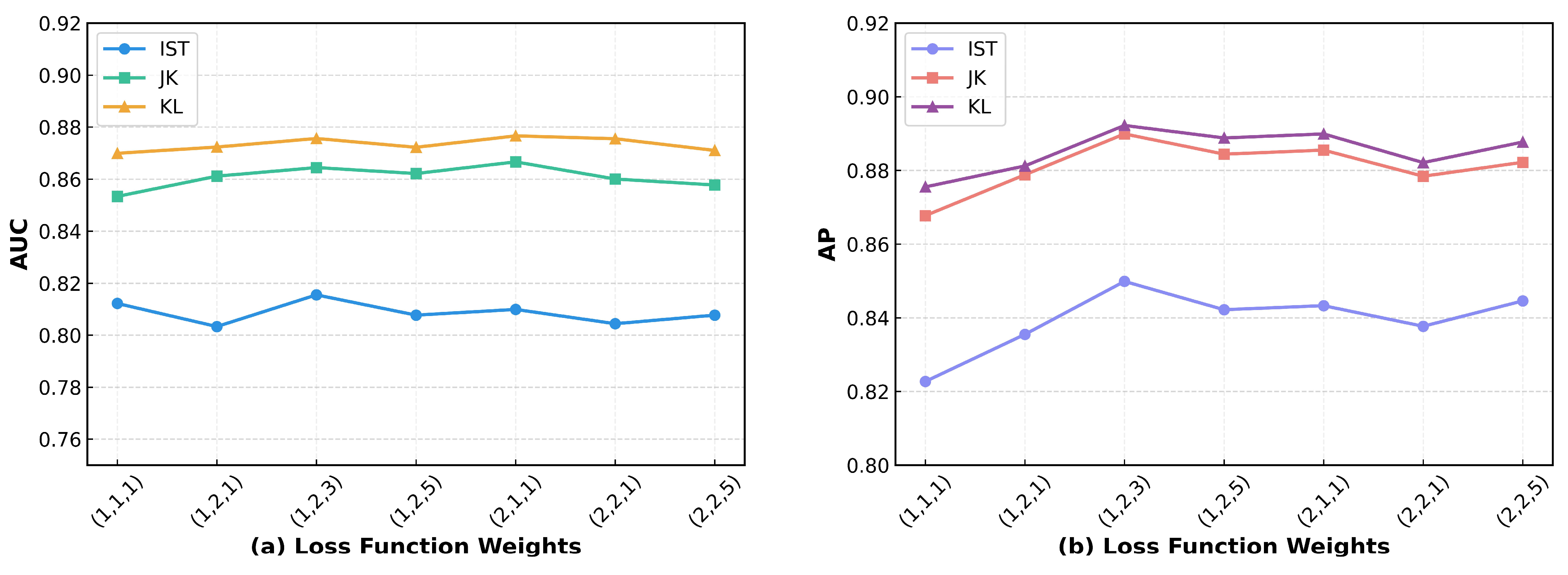
5.8. Hyperparameter Tuning Experiment

We use grid search to obtain the optimal hyperparameter configuration. Then, we fix the remaining hyperparameters and individually adjust each one, observing its impact on the model’s performance. This helps us to assess the importance of each hyperparameter on model performance, optimize the hyperparameter selection process, and enhance the model’s robustness and usability.
For model performance optimization, we design a series of hyperparameter tuning experiments to explore the impact of learning rate, model depth, the number of attention heads, and loss function weights on performance. The experiments are conducted on three representative and diverse datasets: JK, IST, and KL. The experimental results are summarized as follows:
As shown in Figure 8, when investigating the impact of the learning rate on the model, we find that a learning rate of 1 × 10⁻⁴ significantly improves the AUC and AP metrics, allowing the model to quickly converge to a high-performance state, making it the optimal choice. A learning rate of 1 × 10⁻⁵ shows limited performance improvement, while 1 × 10⁻⁶ is too low, leading to poor training results and almost no improvement in model performance.
As shown in Figure 9, when investigating the impact of the number of propagation layers on the model, both the AUC and AP metrics reach high and stable performance levels for the KL, IST, and JK datasets when the number of propagation layers is set to 3. Too few layers lead to insufficient feature extraction, while the 3-layer setup allows for the sufficient capture of data features. Increasing the layers beyond 3 may cause overfitting, increase computational complexity, and offer limited performance improvement. Therefore, the 3-layer propagation configuration is the optimal choice for balancing model performance and resource consumption.
As shown in Figure 10, when investigating the impact of the number of attention heads in the model’s attention mechanism, we find that the KL dataset is insensitive to the configuration of the number of heads, with stable and good performance at 4 heads; the IST dataset exhibits significant dependence on the number of heads, reaching peak AUC and AP at 4 heads; the JK dataset’s performance improves with an increasing number of heads, being optimal at 8 heads, but nearly reaching the peak at 4 heads. Overall, a 4-head configuration effectively balances the performance across the KL, IST, and JK datasets, making it the optimal strategy for enhancing the model’s prediction performance across different datasets.
As shown in Figure 11, when exploring the impact of loss function weight values on the model, we find that adjusting the weight significantly affects AP, while having a smaller impact on AUC. Properly increasing the weight of the KL divergence loss can improve AP, but excessive adjustment harms convergence. After balancing the relationship between model performance improvement and convergence stability, the optimal loss weight configuration is determined as follows: binary cross-entropy loss weight, reconstruction loss weight, and KL divergence loss weight. This configuration ensures good model convergence while maximizing AP performance.

6. Conclusions and Future Work

Due to the difficulty of traditional methods in effectively handling the complex spatiotemporal information in LBSNs and the limitations imposed by high-dimensional redundancy and noise in the data, we propose a Heterogeneous Graph Attention Network (GEVEHGAN) based on Lite-GRU embedding and VAE enhancement for friend link prediction. This model integrates Skip-Gram and Lite-GRU to deeply mine spatiotemporal information in LBSNs and construct efficient feature representations. The VAE module plays a key role in dimensionality reduction, optimizing data dimensions and information representation, and reducing the interference of redundancy and noise on the model. The introduction of edge-level attention mechanisms allows the model to focus precisely on the edge information in the heterogeneous graph that has a significant impact on friend link prediction, significantly improving the model’s performance. Experimental results fully demonstrate the superiority of this model in key metrics such as accuracy and recall rate.
However, the model still has some limitations. It does not explicitly model the multi-hop propagation mechanism of social influence, which may lead to a limited scope of recommendations. Additionally, it mainly focuses on location check-in behavior and does not cover other social network features such as text interactions or user comments, which may affect the model’s generalization ability. Furthermore, privacy risks and data misuse are significant ethical concerns in LBSN tasks. When using LBSN data, privacy protection regulations should be followed, ensuring data de-identification and encryption to avoid unethical behaviors such as excessive commercialization or manipulation.
Future research will explore more refined feature fusion strategies to fully leverage the multi-dimensional information in LBSNs. GEVEHGAN will be applied to practical scenarios such as personalized recommendation and social network influence analysis to verify its broad applicability, providing a new perspective for research in the LBSN field.
In summary, the GEVEHGAN model has significant theoretical and practical value in friend link prediction within location-based social networks. We look forward to achieving more significant results in related fields through continuous optimization and expansion of the GEVEHGAN model.

Author Contributions

Conceptualization, Z.Y. and B.L.; methodology, Z.Y.; validation, Y.W.; formal analysis, Z.Y. and B.L.; investigation, Y.W.; resources, A.L.; data curation, Y.W.; writing—original draft preparation, Z.Y.; writing—review and editing, A.L.; visualization, Z.Y. and B.L.; supervision, A.L.; project administration, Z.Y. and Y.W. All authors have read and agreed to the published version of the manuscript.

Funding

This research received no external funding.

Institutional Review Board Statement

Not applicable.

Informed Consent Statement

Not applicable.

Data Availability Statement

The Foursquare dataset used in this study can be accessed at https://sites.google.com/site/yangdingqi/home/foursquare-dataset (accessed on 15 August 2024).

Acknowledgments

Thanks to Ma Yesen for providing the GPU for model training.

Conflicts of Interest

The authors declare no conflicts of interest.

References

  1. Liben-Nowell, D.; Kleinberg, J. The Link Prediction Problem for Social Networks. In Proceedings of the Twelfth International Conference on Information and Knowledge Management, New Orleans, LA, USA, 3–8 November 2003; ACM: New York, NY, USA; pp. 556–559. [Google Scholar]
  2. Gu, J. Research on Precision Marketing Strategy and Personalized Recommendation Method Based on Big Data Drive. Wirel. Commun. Mob. Comput. 2022, 2022, 6751413. [Google Scholar] [CrossRef]
  3. Chen, Y.-C.; Huang, H.-H.; Chiu, S.-M.; Lee, C. Joint Promotion Partner Recommendation Systems Using Data from Location-Based Social Networks. ISPRS Int. J. Geo-Inf. 2021, 10, 57. [Google Scholar] [CrossRef]
  4. MacPhail, A.; Tannehill, D.; Ataman, R. The Role of the Critical Friend in Supporting and Enhancing Professional Learning and Development. Prof. Dev. Educ. 2024, 50, 597–610. [Google Scholar] [CrossRef]
  5. Chen, J.; Zhang, W. A Review of Research on Location-Based Social Network Point of Interest Recommendation Systems. J. Front. Comput. Sci. Technol. 2022, 16, 1462–1478. [Google Scholar] [CrossRef]
  6. Newman, M.E.J. Clustering and Preferential Attachment in Growing Networks. Phys. Rev. E 2001, 64, 025102. [Google Scholar] [CrossRef] [PubMed]
  7. Tong, H.; Faloutsos, C.; Pan, J. Fast Random Walk with Restart and Its Applications. In Proceedings of the Sixth International Conference on Data Mining (ICDM’06), Hong Kong, China, 18–22 December 2006; IEEE: Hong Kong, China; pp. 613–622. [Google Scholar]
  8. Liu, W.; Lü, L. Link Prediction Based on Local Random Walk. Europhys. Lett. 2010, 89, 58007. [Google Scholar] [CrossRef]
  9. Wang, C.; Satuluri, V.; Parthasarathy, S. Local Probabilistic Models for Link Prediction. In Proceedings of the Seventh IEEE International Conference on Data Mining (ICDM 2007), Omaha, NE, USA, 28–31 October 2007; IEEE: Los Alamitos, CA, USA; pp. 322–331. [Google Scholar]
  10. Neville, J. Statistical Models and Analysis Techniques for Learning in Relational Data; University of Massachusetts Amherst: Amherst, MA, USA, 2006. [Google Scholar]
  11. Yu, K.; Chu, W.; Yu, S.; Tresp, V.; Xu, Z. Stochastic Relational Models for Discriminative Link Prediction. Adv. Neural Inf. Process. Syst. 2006, 19, 1553–1560. [Google Scholar]
  12. Du, Y.; Zheng, Y.; Lee, K.; Zhe, S. Probabilistic Streaming Tensor Decomposition. In Proceedings of the 2018 IEEE International Conference on Data Mining (ICDM), Sentosa, Singapore, 17–20 November 2018; IEEE: Los Angeles, CA, USA; pp. 99–108. [Google Scholar]
  13. Sarukkai, R.R. Link Prediction and Path Analysis Using Markov Chains. Comput. Netw. 2000, 33, 377–386. [Google Scholar] [CrossRef]
  14. Li, X.; Du, N.; Li, H.; Li, K.; Gao, J.; Zhang, A. A Deep Learning Approach to Link Prediction in Dynamic Networks. In Proceedings of the 2014 SIAM International Conference on Data Mining, Philadelphia, PA, USA, 28 April 2014; Society for Industrial and Applied Mathematics: Philadelphia, PA, USA; pp. 289–297. [Google Scholar]
  15. Wang, X.-W.; Chen, Y.; Liu, Y.-Y. Link Prediction through Deep Generative Model. Iscience 2020, 23, 101626. [Google Scholar] [CrossRef]
  16. Wang, H.; Shi, X.; Yeung, D.-Y. Relational Deep Learning: A Deep Latent Variable Model for Link Prediction. In Proceedings of the AAAI Conference on Artificial Intelligence, Philadelphia, PA, USA, 25 February–4 March 2025; Volume 31. [Google Scholar]
  17. Schlichtkrull, M.; Kipf, T.N.; Bloem, P.; Van Den Berg, R.; Titov, I.; Welling, M. Modeling Relational Data with Graph Convolutional Networks. In The Semantic Web; Gangemi, A., Navigli, R., Vidal, M.-E., Hitzler, P., Troncy, R., Hollink, L., Tordai, A., Alam, M., Eds.; Lecture Notes in Computer Science; Springer International Publishing: Cham, Switzerland, 2018; Volume 10843, pp. 593–607. ISBN 978-3-319-93416-7. [Google Scholar]
  18. Kipf, T.N.; Welling, M. Variational Graph Auto-Encoders 2016. arXiv 2016, arXiv:1611.07308. [Google Scholar]
  19. Scarselli, F.; Gori, M.; Tsoi, A.C.; Hagenbuchner, M.; Monfardini, G. The Graph Neural Network Model. IEEE Trans. Neural Netw. 2008, 20, 61–80. [Google Scholar] [CrossRef] [PubMed]
  20. Wu, Y.; Lian, D.; Jin, S.; Chen, E. Graph Convolutional Networks on User Mobility Heterogeneous Graphs for Social Relationship Inference. In Proceedings of the Twenty-Eighth International Joint Conference on Artificial Intelligence Main Track, Macau, China, 10–16 August 2019; pp. 3898–3904. [Google Scholar]
  21. Backes, M.; Humbert, M.; Pang, J.; Zhang, Y. Walk2friends: Inferring Social Links from Mobility Profiles. In Proceedings of the 2017 ACM SIGSAC Conference on Computer and Communications Security, Dallas, TX, USA, 30 October–3 November 2017; ACM: New York, NY, USA; pp. 1943–1957. [Google Scholar]
  22. Zhang, W.; Lai, X.; Wang, J. Social Link Inference via Multiview Matching Network from Spatiotemporal Trajectories. IEEE Trans. Neural Netw. Learn. Syst. 2020, 34, 1720–1731. [Google Scholar] [CrossRef]
  23. Hamilton, W.; Ying, Z.; Leskovec, J. Inductive Representation Learning on Large Graphs. Adv. Neural Inf. Process. Syst. 2017, 30. [Google Scholar] [CrossRef]
  24. Velickovic, P.; Cucurull, G.; Casanova, A.; Romero, A.; Lio, P.; Bengio, Y. Graph Attention Networks. Stat 2017, 1050. [Google Scholar] [CrossRef]
  25. Wang, X.; Ji, H.; Shi, C.; Wang, B.; Ye, Y.; Cui, P.; Yu, P.S. Heterogeneous Graph Attention Network. In Proceedings of the The World Wide Web Conference, San Francisco, CA, USA, 13–17 May 2019; ACM: New York, NY, USA; pp. 2022–2032. [Google Scholar]
  26. Hu, Q.; Lin, W.; Tang, M.; Jiang, J. Mbhan: Motif-Based Heterogeneous Graph Attention Network. Appl. Sci. 2022, 12, 5931. [Google Scholar] [CrossRef]
  27. Zhou, X.; Wang, Z.; Liu, X.; Liu, Y.; Sun, G. An Improved Context-Aware Weighted Matrix Factorization Algorithm for Point of Interest Recommendation in LBSN. Inf. Syst. 2024, 122, 102366. [Google Scholar] [CrossRef]
  28. Seo, Y.-D.; Cho, Y.-S. Point of Interest Recommendations Based on the Anchoring Effect in Location-Based Social Network Services. Expert Syst. Appl. 2021, 164, 114018. [Google Scholar] [CrossRef]
  29. Wang, C.; Yuan, M.; Zhang, R.; Peng, K.; Liu, L. Efficient Point-of-Interest Recommendation Services with Heterogenous Hypergraph Embedding. IEEE Trans. Serv. Comput. 2022, 16, 1132–1143. [Google Scholar] [CrossRef]
  30. Nguyen, H.T.; Tran, C.L.H.; Luong, H.H. Mobility Prediction on a Location-Based Social Network Using K Latest Movements of Friends. In Intelligent Systems and Networks; Anh, N.L., Koh, S.-J., Nguyen, T.D.L., Lloret, J., Nguyen, T.T., Eds.; Lecture Notes in Networks and Systems; Springer Nature Singapore: Singapore, 2022; Volume 471, pp. 279–286. ISBN 978-981-19-3393-6. [Google Scholar]
  31. Li, Y.; Fan, Z.; Zhang, J.; Shi, D.; Xu, T.; Yin, D.; Deng, J.; Song, X. Heterogeneous Hypergraph Neural Network for Friend Recommendation with Human Mobility. In Proceedings of the 31st ACM International Conference on Information & Knowledge Management, Atlanta, GA, USA, 17–21 October 2022; ACM: New York, NY, USA; pp. 4209–4213. [Google Scholar]
  32. Li, Y.; Fan, Z.; Yin, D.; Jiang, R.; Deng, J.; Song, X. HMGCL: Heterogeneous Multigraph Contrastive Learning for LBSN Friend Recommendation. World Wide Web 2023, 26, 1625–1648. [Google Scholar] [CrossRef]
  33. Yang, L.; Marmolejo Duarte, C.R.; Martí Ciriquiá, P. Exploring the Applications and Limitations of Location-Based Social Network Data in Urban Spatiotemporal Analysis. Ph.D. Thesis, Universitat Politècnica de Catalunya, Barcelona, Spain, 2021. [Google Scholar]
  34. Laman, H.; Eluru, N.; Yasmin, S. Using Location-Based Social Network Data for Activity Intensity Analysis. J. Transp. Land Use 2019, 12, 723–740. [Google Scholar] [CrossRef]
  35. Nolasco-Cirugeda, A.; García-Mayor, C. Social Dynamics in Cities: Analysis through LBSN Data. Procedia Comput. Sci. 2022, 207, 877–886. [Google Scholar] [CrossRef]
  36. Xu, D.; Chen, Y.; Cui, N.; Li, J. Towards Multi-Dimensional Knowledge-Aware Approach for Effective Community Detection in LBSN. World Wide Web 2023, 26, 1435–1458. [Google Scholar] [CrossRef]
  37. Wang, K.; Wang, X.; Lu, X. POI Recommendation Method Using LSTM-Attention in LBSN Considering Privacy Protection. Complex Intell. Syst. 2023, 9, 2801–2812. [Google Scholar] [CrossRef]
  38. Sun, L.; Zheng, Y.; Lu, R.; Zhu, H.; Zhang, Y. Towards Privacy-Preserving Category-Aware POI Recommendation over Encrypted LBSN Data. Inf. Sci. 2024, 662, 120253. [Google Scholar] [CrossRef]
  39. Sai, A.M.V.V.; Zhang, K.; Li, Y. User Motivation Based Privacy Preservation in Location Based Social Networks. In Proceedings of the 2021 IEEE SmartWorld, Ubiquitous Intelligence & Computing, Advanced & Trusted Computing, Scalable Computing & Communications, Internet of People and Smart City Innovation (SmartWorld/SCALCOM/UIC/ATC/IOP/SCI), Atlanta, GA, USA, 18–21 October 2021; IEEE: Los Alamitos, CA, USA; pp. 471–478. [Google Scholar]
  40. Jaccard, P. Distribution de La Flore Alpine Dans Le Bassin Des Dranses et Dans Quelques Régions Voisines. Bull Soc. Vaudoise. Sci. Nat. 1901, 37, 241–272. [Google Scholar]
  41. Adamic, L.A.; Adar, E. Friends and Neighbors on the Web. Soc. Netw. 2003, 25, 211–230. [Google Scholar] [CrossRef]
  42. Barabâsi, A.-L.; Jeong, H.; Néda, Z.; Ravasz, E.; Schubert, A.; Vicsek, T. Evolution of the Social Network of Scientific Collaborations. Phys. Stat. Mech. Its Appl. 2002, 311, 590–614. [Google Scholar] [CrossRef]
  43. Zhou, T.; Lü, L.; Zhang, Y.-C. Predicting Missing Links via Local Information. Eur. Phys. J. B 2009, 71, 623–630. [Google Scholar] [CrossRef]
  44. Salton, G. Modern Information Retrieval; McGraw-Hill Education: New York, NY, USA, 1983. [Google Scholar]
  45. Lü, L.; Jin, C.-H.; Zhou, T. Similarity Index Based on Local Paths for Link Prediction of Complex Networks. Phys. Rev. E 2009, 80, 046122. [Google Scholar] [CrossRef]
  46. Katz, L. A New Status Index Derived from Sociometric Analysis. Psychometrika 1953, 18, 39–43. [Google Scholar] [CrossRef]
  47. Rafiee, S.; Salavati, C.; Abdollahpouri, A. CNDP: Link Prediction Based on Common Neighbors Degree Penalization. Phys. Stat. Mech. Its Appl. 2020, 539, 122950. [Google Scholar] [CrossRef]
  48. Yuliansyah, H.; Othman, Z.A.; Bakar, A.A. A New Link Prediction Method to Alleviate the Cold-Start Problem Based on Extending Common Neighbor and Degree Centrality. Phys. Stat. Mech. Its Appl. 2023, 616, 128546. [Google Scholar] [CrossRef]
  49. Aziz, F.; Gul, H.; Muhammad, I.; Uddin, I. Link Prediction Using Node Information on Local Paths. Phys. Stat. Mech. Its Appl. 2020, 557, 124980. [Google Scholar] [CrossRef]
  50. Ayoub, J.; Lotfi, D.; El Marraki, M.; Hammouch, A. Accurate Link Prediction Method Based on Path Length between a Pair of Unlinked Nodes and Their Degree. Soc. Netw. Anal. Min. 2020, 10, 9. [Google Scholar] [CrossRef]
  51. Kipf, T.N.; Welling, M. Semi-Supervised Classification with Graph Convolutional Networks. arXiv 2017, arXiv:1609.02907. [Google Scholar]
  52. He, X.; Deng, K.; Wang, X.; Li, Y.; Zhang, Y.; Wang, M. LightGCN: Simplifying and Powering Graph Convolution Network for Recommendation. In Proceedings of the 43rd International ACM SIGIR Conference on Research and Development in Information Retrieval, Virtual Event, China, 25–30 July 2020; ACM: New York, NY, USA; pp. 639–648. [Google Scholar]
  53. Chen, L.; Xie, Y.; Zheng, Z.; Zheng, H.; Xie, J. Friend Recommendation Based on Multi-Social Graph Convolutional Network. IEEE Access 2020, 8, 43618–43629. [Google Scholar] [CrossRef]
  54. van den Berg, R.; Kipf, T.N.; Welling, M. Graph Convolutional Matrix Completion 2017. arXiv 2017, arXiv:1706.02263. [Google Scholar]
  55. Zhang, C.; Song, D.; Huang, C.; Swami, A.; Chawla, N.V. Heterogeneous Graph Neural Network. In Proceedings of the 25th ACM SIGKDD International Conference on Knowledge Discovery & Data Mining, Anchorage, AK, USA, 25 July 2019; ACM: New York, NY, USA; pp. 793–803. [Google Scholar]
  56. Dong, Y.; Chawla, N.V.; Swami, A. Metapath2vec: Scalable Representation Learning for Heterogeneous Networks. In Proceedings of the 23rd ACM SIGKDD International Conference on Knowledge Discovery and Data Mining, Halifax, NS, Canada, 13–17 August 2017; ACM: New York, NY, USA; pp. 135–144. [Google Scholar]
  57. Fu, X.; Zhang, J.; Meng, Z.; King, I. MAGNN: Metapath Aggregated Graph Neural Network for Heterogeneous Graph Embedding. In Proceedings of the Web Conference 2020, Taipei, Taiwan, 20–24 April 2020; ACM: New York, NY, USA; pp. 2331–2341. [Google Scholar]
  58. Fan, Y.; Ju, M.; Zhang, C.; Zhao, L.; Ye, Y. Heterogeneous Temporal Graph Neural Network 2021. arXiv 2021, arXiv:2110.13889. [Google Scholar]
  59. Salamat, A.; Luo, X.; Jafari, A. HeteroGraphRec: A Heterogeneous Graph-Based Neural Networks for Social Recommendations. Knowl.-Based Syst. 2021, 217, 106817. [Google Scholar] [CrossRef]
  60. Shao, Y.; Liu, C. H2Rec: Homogeneous and Heterogeneous Network Embedding Fusion for Social Recommendation. Int. J. Comput. Intell. Syst. 2021, 14, 1303–1314. [Google Scholar] [CrossRef]
  61. Yadati, N.; Nimishakavi, M.; Yadav, P.; Nitin, V.; Louis, A.; Talukdar, P. Hypergcn: A New Method for Training Graph Convolutional Networks on Hypergraphs. Adv. Neural Inf. Process. Syst. 2019, 32. [Google Scholar] [CrossRef]
  62. Dong, Y.; Sawin, W.; Bengio, Y. HNHN: Hypergraph Networks with Hyperedge Neurons 2020. arXiv 2020, arXiv:2006.12278. [Google Scholar]
  63. Feng, Y.; You, H.; Zhang, Z.; Ji, R.; Gao, Y. Hypergraph Neural Networks. In Proceedings of the AAAI Conference on Artificial Intelligence, Honolulu, HI, USA, 27 January–1 February 2019; Volume 33, pp. 3558–3565. [Google Scholar]
  64. Huang, J.; Yang, J. UniGNN: A Unified Framework for Graph and Hypergraph Neural Networks 2021. arXiv 2021, arXiv:2105.00956. [Google Scholar]
  65. Chien, E.; Pan, C.; Peng, J.; Milenkovic, O. You Are AllSet: A Multiset Function Framework for Hypergraph Neural Networks 2022. arXiv 2022, arXiv:2106.13264. [Google Scholar]
  66. Mikolov, T.; Chen, K.; Corrado, G.; Dean, J. Efficient Estimation of Word Representations in Vector Space 2013. arXiv 2013, arXiv:1301.3781. [Google Scholar]
  67. Ravanelli, M.; Brakel, P.; Omologo, M.; Bengio, Y. Light Gated Recurrent Units for Speech Recognition. IEEE Trans. Emerg. Top. Comput. Intell. 2018, 2, 92–102. [Google Scholar] [CrossRef]
  68. Brody, S.; Alon, U.; Yahav, E. How Attentive Are Graph Attention Networks? arXiv 2022, arXiv:2105.14491. [Google Scholar]
  69. Li, G.; Muller, M.; Thabet, A.; Ghanem, B. Deepgcns: Can Gcns Go as Deep as Cnns? In Proceedings of the IEEE/CVF International Conference on Computer Vision, Seoul, Republic of Korea, 27 October–2 November 2019; pp. 9267–9276. [Google Scholar]
  70. Li, G.; Xiong, C.; Thabet, A.; Ghanem, B. DeeperGCN: All You Need to Train Deeper GCNs 2020. arXiv 2020, arXiv:2006.07739. [Google Scholar]
  71. Lv, Q.; Ding, M.; Liu, Q.; Chen, Y.; Feng, W.; He, S.; Zhou, C.; Jiang, J.; Dong, Y.; Tang, J. Are We Really Making Much Progress?: Revisiting, Benchmarking and Refining Heterogeneous Graph Neural Networks. In Proceedings of the 27th ACM SIGKDD Conference on Knowledge Discovery & Data Mining, Virtual Event, Singapore, 14–18 August 2021; ACM: New York, NY, USA; pp. 1150–1160. [Google Scholar]
  72. Wu, J.; Hu, R.; Li, D.; Ren, L.; Hu, W.; Xiao, Y. Where Have You Been: Dual Spatiotemporal-Aware User Mobility Modeling for Missing Check-in POI Identification. Inf. Process. Manag. 2022, 59, 103030. [Google Scholar] [CrossRef]
Figure 1. GEVEHAN architecture diagram, including five components: (1) construct a heterogeneous graph with two types of nodes and three types of edges based on LBSN user check-in trajectory information; (2) learn POI embeddings using the Skip-Gram model, and user embeddings using Lite-GRU, to initialize the nodes; (3) use the VAE module for dimensionality reduction and denoising; (4) apply edge-level attention, multi-head attention mechanism, and residual connections for feature aggregation and update; (5) perform friend link prediction using cosine similarity. The relationships are as follows: a, b, and c are friends; a, t, c, and t are not friends.
Applsci 15 04585 g001
Figure 2. Schematic of user trajectories. Different colors represent different users, while solid and dashed lines represent different sub-trajectories of the same user. On one day, a went to school, b went to the shop and bar, and c went to school. On another day, a went to the gym, b went to the restaurant and gym, and c went to the hospital and company, t hasn’t gone anywhere in the past two days.
Applsci 15 04585 g002
Figure 3. Basic framework of VAE, consisting of three parts: encoder, latent variables, and decoder. The encoder maps the input data to the latent space, the decoder generates reconstructed data based on the latent variables, and the entire process is achieved by optimizing the variational lower bound.
Applsci 15 04585 g003
Figure 4. Performance comparison of eight recommendation models on six different datasets—analysis of AUC, AP, and TOP@10 metrics. (a) Shows the AUC performance of the eight recommendation models across six datasets. (b) Shows the AP performance of each model on the same datasets. (c) Shows the TOP@10 hit rate performance of these models across six datasets. With these metrics, we can comprehensively evaluate the strengths and weaknesses of each recommendation model in different scenarios.
Applsci 15 04585 g004
Figure 5. Performance evaluation metrics of GEVEHGAN and its derived models on the NYC and TKY datasets. (a) Shows the AUC scores of GEVEHGAN and its derived models on the NYC and TKY datasets; (b) displays the average precision scores of these models on the two city datasets; (c) presents the TOP@10 hit rate of the models on the NYC and TKY datasets. Through these detailed metric comparisons, we can gain a deeper understanding of the performance differences of GEVEHGAN and its variants in different data environments.
Applsci 15 04585 g005
Figure 6. The change trends of AUC, AP, and loss with respect to epoch for GEVEHGAN on six datasets. (af), respectively, show the improvement in AUC and AP, and the decrease in loss, with the increase in training epochs on the IST, JK, KL, NYC, SP, and TKY datasets.
Applsci 15 04585 g006
Figure 7. The trend of the Top@K metric of GEVEHGAN across six datasets with the training epochs. (af), respectively, depict how the Top@K performance of the GEVEHGAN model evolves as the number of training epochs increases on the IST, JK, KL, NYC, SP, and TKY datasets.
Applsci 15 04585 g007
Figure 8. Analysis of the impact of learning rate on model performance metrics. (ac) show the changes in the AUC metric with epochs for the GEVEHGAN model on the KL, JK, and IST datasets at different learning rates (1 × 10⁻⁴, 1 × 10⁻⁵, 1 × 10⁻⁶). (df) display the changes in the AP metric with training epochs for these three datasets under the same learning rate settings.
Applsci 15 04585 g008
Figure 9. Analysis of the impact of propagation layers on model performance metrics. (a) shows how the AUC metric of the GEVEHGAN model changes with the increase in propagation layers on the KL, JK, and IST datasets; (b) displays the trend of the model’s AP metric as the number of propagation layers changes on these three datasets.
Applsci 15 04585 g009
Figure 10. The impact of the number of attention heads in the multi-head attention mechanism on model performance metrics. (a) shows the trend of the AUC metric as the number of attention heads changes in the GEVEHGAN model on the KL, JK, and IST datasets; (b) shows the trend of the AP metric as the number of attention heads changes in these three datasets.
Applsci 15 04585 g010
Figure 11. Analysis of the impact of loss function weight values on model performance metrics. (a) shows the trend of the AUC metric of the GEVEHGAN model with varying loss function weight values on the KL, JK, and IST datasets; (b) displays the trend of the model’s AP metric with varying loss function weight values on these three datasets.
Applsci 15 04585 g011
Table 1. Statistics of dataset after pretreatment.
DatasetUser NumberPOI NumberCheck-In NumberFriends NumberAverage Sign-In Count
NYC37543626104,99112,09827.97
TKY716610,856698,88957,14297.53
SP38116255247,68316,36364.99
JK61848805376,07617,79860.81
IST999312,608884,31345,00288.49
KL632410,804524,06134,53782.87
Table 2. GEVEHGAN experimental environment configuration.
Experiment EnvironmentSpecific Configuration
Operating SystemWindows 11 64-bit OS
CPU12th Gen Intel(R) Core(TM) i7-12700H 2.30 GHz
GPUNVIDIA GeForce RTX 3080
Memory64 GB
Programming LanguagePython 3.10
Deep Learning FrameworkPyTorch 1.12
Library Versionsnumpy = 1.13.1, scikit-learn = 1.0.2, dgl = 0.7.2
Table 3. GEVEHGAN model parameter setting table.
Parameter NameParameter DescriptionParameter Value
Window sizeSkip-Gram window size10
Initial embedding dimInitial embedding dimension size64
Lite-GRU num layersLite-GRU layer number1
Node embedding dimNode feature mapping dimension128
Edge embedding dimEdge feature mapping dimension10
σ (·)Nonlinear activation functionReLU(·)
LearnAdam optimizer learning rate0.001
EpochsIterations2700
GNN num layersGNN layer number3
KMultiple attention number4
Window sizeSkip-Gram window size10
Disclaimer/Publisher’s Note: The statements, opinions and data contained in all publications are solely those of the individual author(s) and contributor(s) and not of MDPI and/or the editor(s). MDPI and/or the editor(s) disclaim responsibility for any injury to people or property resulting from any ideas, methods, instructions or products referred to in the content.

