Abstract
This paper presents a lightweight fault diagnosis framework for bearing defects, integrating time-frequency analysis, deep learning, and model compression techniques to address challenges in resource-constrained environments. The proposed method combines the S-transform for high-resolution time-frequency representation with MobileNet as an efficient backbone network, enabling robust feature extraction from complex vibration signals. To enhance deployment on edge devices, knowledge distillation is employed to compress the model, significantly reducing computational complexity while maintaining diagnostic accuracy. Additionally, domain adaptation is considered to mitigate domain shift issues, ensuring robust performance across varying operating conditions. Experimental results demonstrate the framework’s effectiveness, achieving high diagnostic accuracy with reduced computational overhead, making it a practical solution for real-time industrial applications. The proposed approach bridges the gap between advanced deep learning techniques and practical industrial requirements, offering a scalable and efficient solution for bearing fault diagnosis.
1. Introduction
1.1. Background
Bearing fault diagnosis plays a critical role for the reliability and safety of rotating machinery. As one of the most important components, bearing failures would lead to catastrophic breakdowns, costly downtime, and even safety hazards. Traditional fault diagnosis methods often rely on signal processing techniques, such as Fourier transform or wavelet analysis, to extract fault-related features from vibration signals. However, these methods typically require extensive domain expertise and may struggle to handle complex, non-stationary signals. With the rapid development of deep learning, data-driven approaches have shown great potential in automatically learning discriminative features from raw data. Despite their success, deep learning models often suffer from high computational complexity and large memory requirements, making them challenging to deploy in resource-constrained environments, such as edge devices or embedded systems.
1.2. Related Work
Edge computing for fault diagnosis. Edge computing has emerged as a critical paradigm for enabling real-time data processing and decision-making in industrial applications, particularly in the context of fault diagnosis []. Traditional fault diagnosis systems often rely on cloud-based solutions, where data are transmitted to remote servers for analysis []. However, this approach introduces latency, bandwidth limitations, and privacy concerns, making it unsuitable for time-sensitive applications, such as bearing fault diagnosis []. Edge computing addresses these challenges by bringing computation and data storage closer to the data source, enabling real-time analysis and decision-making at the edge of the network. In the context of bearing fault diagnosis, edge computing allows for the deployment of lightweight diagnostic models directly on industrial machinery, facilitating immediate detection and response to faults. Recent studies have explored the integration of edge computing with machine learning techniques for fault diagnosis []. For instance, Wang et al. proposed a lightweight reprogramming framework for cross-device fault diagnosis, which includes cloud-based C-model training and edge-based E-model reprogramming and application stages []. Similarly, Peng et al. proposed a fault location scheme for distribution grids by utilizing edge computing, which is aimed at ensuring data privacy and security []. These works highlight the potential of edge computing to revolutionize fault diagnosis by enabling real-time, on-device analysis while reducing reliance on centralized cloud infrastructure. There are also related studies that have proposed a data augmentation method combining continuous wavelet transform and a deep convolutional generative adversarial network (DCGAN), as well as a hybrid data-driven scheme combined with physics-based sample generation (PSG), which have made contributions to the lightweighting of the fault diagnosis model [,].
Model Compression. Model compression has become a crucial research area in deep learning, particularly for applications requiring deployment on resource-constrained devices such as edge nodes. The main goal of model compression is to reduce the storage size and computational complexity of the neural networks while maintaining the calculation performance. The model compression techniques include pruning [], quantization, and knowledge distillation. Pruning involves removing redundant parameters and kernels on the neural networks, thereby decreasing model storage and improving model inference speed [,]. Parameter quantization reduces the precision of model weights and activations, typically from 32-bit floats to lower-bit such as 8-bit integers. It decreases memory usage and computational costs, enabling efficient deployment on resource-limited devices []. As one of the most popular techniques, knowledge distillation constructs a compact student model which achieves comparable performance from a complex teacher model by learning from its soft targets. In the context of bearing fault diagnosis, knowledge distillation has been widely adopted to compress deep learning models for edge deployment []. For instance, Fu et al. applied knowledge distillation to compress a 1D convolutional neural network (1DCNN) for bearing fault diagnosis, achieving a significant reduction in model size without sacrificing accuracy []. In [], a student network is introduced to learn diagnostic features from a larger teacher network with a learnable embedding in the attention mechanism. It is beneficial to new operating conditions via a joint classifier.
Domain Adaptation for Cross-Domain Diagnosis. In bearing fault diagnosis, operating conditions such as load, speed, and environmental noise can vary significantly []. Thus, the domain shift would occur when the distribution of data in the target domain differs from that in the source domain, thereby degrading the model performance. To overcome this, domain adaptation techniques are necessary to align the feature distributions of the source and target domains, enabling models to generalize across different conditions []. Tang et al. introduced a domain adaptation method which employs the Joint Maximum Mean Discrepancy and Conditional Adversarial Domain Adaption Network, to align feature distributions across domains []. Zhang et al. proposed a tailored dynamic conditional adversarial domain adaptation mode for cross-domain fault diagnosis, achieving accuracy and stability for wind turbine gearbox fault diagnosis []. These techniques collectively address the challenge of domain shift, enabling robust fault diagnosis across diverse operating conditions.
1.3. Challenges
Although previous research has achieved outstanding successes, there still exist several challenges as follows:
- The ability to combine signal processing with deep learning lies in the effective extraction and utilization of discriminative features from raw signals. Traditional signal processing methods, such as Fourier transform and wavelet analysis, often require extensive domain expertise and may struggle to handle complex, non-stationary signals. While deep learning models can automatically learn features from raw data, they are highly sensitive to noise and variations in signal quality. Balancing the strengths of both approaches to achieve robust feature extraction remains a critical challenge, especially in real-time applications.
- Deep learning model compression is particularly relevant in resource-constrained environments, such as edge devices or embedded systems. Deep learning models, despite their high diagnostic accuracy, often suffer from high computational complexity and large memory requirements, making them difficult to deploy in practical industrial settings. Techniques like pruning, quantization, and knowledge distillation are commonly used to compress models, but these methods often lead to a trade-off between model size and diagnostic performance. Ensuring that compressed models retain their generalization capabilities while reducing computational overhead is a non-trivial task, especially when dealing with complex fault patterns.
- Cross-domain diagnosis and domain adaptation arises from the inherent differences between source and target domains. In real-world industrial scenarios, the distribution of data can vary significantly due to changes in operating conditions, such as load, speed, and environmental noise. This domain shift can severely degrade the performance of fault diagnosis models trained on one domain when applied to another. Domain adaptation techniques aim to align the feature distributions of source and target domains, but achieving effective adaptation without extensive labeled data in the target domain remains a major hurdle. Additionally, the dynamic nature of fault patterns across domains further complicates the development of robust and adaptive diagnostic models.
1.4. Contributions
Facing these challenges, model compression techniques, such as parameter quantization, pruning, and knowledge distillation, have emerged as crucial research areas. These techniques aim to reduce the storage size and computational complexity of deep learning models while maintaining their performance. Among these, parameter quantization, which reduces the precision of model weights and activations from 32-bit floating-point to lower-bit representations (e.g., 8-bit integers), has proven effective in decreasing memory usage and computational costs. This enables the deployment of deep learning models on edge devices with limited resources, facilitating real-time fault diagnosis in industrial settings. However, the application of these techniques in bearing fault diagnosis remains underexplored, particularly in scenarios where operating conditions such as load, speed, and environmental noise vary significantly.
Moreover, the issue of domain shift further complicates the deployment of fault diagnosis models. In real-world industrial scenarios, the distribution of data collected under different working conditions can vary significantly, leading to degraded model performance when applied to new domains. Traditional fault diagnosis models trained on data from one set of operating conditions often fail to generalize to new conditions, limiting their practical applicability. Domain adaptation techniques, which aim to align the feature distributions of source and target domains, have shown potential in addressing this challenge. By enabling models to learn domain-invariant features, these techniques can improve the robustness and generalization capabilities of fault diagnosis systems across diverse operating conditions. Motivated by these, a novel lightweight diagnosis framework is proposed for the resource-constrained embedded systems. The main contributions are presented as follows:
- The proposed method introduces a novel combination of the S-transform and MobileNet for bearing fault diagnosis. While the S-transform provides a high-resolution time-frequency representation of vibration signals, capturing both the temporal and spectral characteristics of faults, MobileNet serves as an efficient backbone network for feature extraction. This integration leverages the strengths of signal processing and deep learning, enabling the model to extract discriminative features from complex vibration data. Unlike traditional methods that rely on handcrafted features or less efficient deep learning architectures, this approach ensures robust fault detection while maintaining computational efficiency, making it suitable for real-time applications.
- A significant innovation in this work is the application of knowledge distillation to compress the MobileNet backbone, addressing the challenge of deploying deep learning models on edge devices with limited computational resources. By training a lightweight student model to mimic the behavior of a larger teacher model, the proposed method achieves a balance between accuracy and efficiency. This approach not only reduces the model’s size and computational complexity but also retains the rich feature representations learned by the teacher model. This innovation is particularly impaction for industrial applications, where real-time fault diagnosis on embedded systems is critical.
- The proposed technical route establishes an end-to-end framework that seamlessly integrates vibration signal acquisition, time-frequency analysis, deep feature extraction, and model compression. Unlike traditional fault diagnosis methods that often require separate stages for feature extraction and classification, this framework unifies the entire process into a cohesive system. The use of MobileNet and knowledge distillation ensures that the framework is not only accurate but also computationally efficient, enabling real-time deployment. This holistic approach represents a significant advancement in bearing fault diagnosis, offering a practical solution for industrial monitoring and maintenance.
1.5. Organization
2. Methodology
2.1. Overall
As shown in Figure 1, the proposed technical route for bearing fault diagnosis involves four key steps: vibration signal acquisition and preprocessing, time-frequency analysis using the S-transform, feature extraction using MobileNet as the backbone network, and model compression using knowledge distillation. This approach leverages the strengths of time-frequency analysis and deep learning to provide an accurate and efficient solution for bearing fault diagnosis. The use of MobileNet as the backbone network ensures that the model is lightweight and suitable for real-time applications, while knowledge distillation further compresses the model, making it deployable on resource-constrained devices. This combination of techniques offers a promising solution for the early detection and diagnosis of bearing faults, which is crucial for preventing catastrophic failures and reducing maintenance costs in industrial applications.
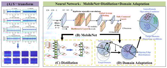
Figure 1.
The main framework of the proposed method.
2.2. Backbone Design
2.2.1. Time-Frequency Analysis Using S-Transform
Vibration signals are widely used in fault diagnosis due to their sensitivity to mechanical anomalies. The signals are typically collected using accelerometers mounted on the bearing housing. The sampling frequency should be chosen carefully to ensure that the relevant frequency components of the bearing faults are captured. For instance, a sampling frequency of at least 10 kHz is often recommended to capture high-frequency components associated with localized defects.
Once the raw vibration signals are acquired, the time-frequency representation using the S-transform is imported. The S-transform is a powerful time-frequency analysis tool that combines the advantages of the Short-Time Fourier Transform (STFT) and the Wavelet Transform. It provides a time-frequency representation that is particularly useful for analyzing non-stationary signals. The S-transform is defined as follows:
where is the vibration signal, is the time shift, and f is the frequency. The S-transform produces a time-frequency matrix that captures the frequency content of the signal. Then, it is used to generate a time-frequency image, which serves as the input to the deep learning model.
The time-frequency image provides a rich representation of the vibration signal, highlighting the presence of fault-related frequency components and their temporal evolution. This representation is particularly useful for detecting and diagnosing bearing faults, as it allows the model to capture both the frequency and temporal characteristics of the fault.
2.2.2. Feature Extraction Using Mobilenet
With the time-frequency images generated, a deep learning model is proposed to extract fault features. In this work, MobileNet is chosen as the backbone network due to its efficiency and effectiveness in image classification. MobileNet is a lightweight convolutional neural network (CNN) designed for mobile and embedded systems. It employs depth-wise separable convolutions, which significantly reduce the number of parameters and computational complexity compared to traditional CNNs, making it suitable for real-time applications.
The MobileNet architecture consists of a series of depth-wise separable convolutional layers, followed by batch normalization and ReLU activation functions. The network is trained to classify the time-frequency images into different fault categories (e.g., normal, inner race fault, outer race fault, ball fault). During training, the network learns to extract discriminative features from the time-frequency images that are indicative of the bearing’s health condition.
The output of the MobileNet backbone is a high-dimensional feature vector that encapsulates the essential information about the bearing’s condition. These features are then passed to a fully connected layer for classification. However, the high dimensionality of the feature vector may lead to increased computational complexity and memory usage, which can be problematic for deployment on resource-constrained devices.
In this study, we propose a lightweight convolutional neural network based on MobileNetV3 for processing time-frequency matrices derived from vibration signals. The input to the network is a time-frequency matrix of size , obtained using the S-transform with a sampling rate of 4096 Hz and a sampling duration of 1 s. The network architecture is designed as follows:
- Input Layer: The input to the network is a single-channel time-frequency matrix of size .
- Initial Convolutional Layer: A convolutional layer with 16 filters of size , stride , and padding ‘same’ is applied, followed by the h-swish activation function. This reduces the spatial dimensions to .
- Bottleneck Layers: A series of bottleneck layers are employed, each consisting of depthwise separable convolutions, Squeeze-and-Excitation (SE) modules, and h-swish activations. The number of output channels in these layers progressively increases from 16 to 160, with intermediate channel sizes of 24, 40, 80, and 112. Strides of are used for downsampling, while strides of maintain spatial resolution.
- Global Average Pooling: A global average pooling layer reduces the spatial dimensions to a vector of size 160.
- Fully Connected Layers: Two fully connected layers with 1024 and 128 neurons, respectively, are applied, each followed by the h-swish activation. The final output layer uses a softmax activation for classification, with the number of neurons equal to the number of classes.
Moreover, in this paper, the MobileNet network is trained using the Adam optimizer with an initial learning rate of 0.001, which decays by a factor of 0.1 every 20 epochs. To ensure sufficient convergence, the model is trained for 100 epochs with a batch size of 32. Moreover, a dropout rate of 0.2 is set in the fully connected layer in order to enhance generalization capability. Furthermore, data augmentation techniques, including random horizontal flipping, cropping, and brightness adjustment, are employed to improve the robustness of the model against overfitting and variations in input data.
2.3. Knowledge Distillation
Knowledge distillation is a powerful technique for model compression, where a smaller, more efficient student model is trained to replicate the behavior of a larger, more complex teacher model. In the context of bearing fault diagnosis, the teacher model is the original MobileNet backbone, which has been trained to classify time-frequency images of vibration signals into different fault categories. The student model, on the other hand, is a compressed version of MobileNet with fewer parameters, designed to achieve similar performance while being more computationally efficient.
The knowledge distillation process involves two main components: the classification loss and the distillation loss. The classification loss ensures that the student model learns to correctly classify the input data, while the distillation loss encourages the student model to mimic the soft predictions of the teacher model. The soft predictions, or soft targets, are the output probabilities produced by the teacher model before applying the final softmax function. These soft targets contain valuable information about the relationships between different classes, which can help the student model generalize better.
The overall loss function for training the student model is a weighted combination of the classification loss and the distillation loss:
where is a trade-off hyperparameter that balances the contributions of the two components. When , the total loss prioritizes supervision from the ground-truth labels, resembling standard supervised training. Conversely, emphasizes knowledge transferred from the teacher model via distillation.
The classification term is defined as the standard cross-entropy between the teacher’s predictions and the ground-truth labels:
where is the true label for the i-th sample, and is the predicted probability for the i-th sample. The distillation loss is the cross-entropy loss between the student model’s predictions and the teacher model’s soft targets:
where is the soft target produced by the teacher model for the i-th sample. The soft targets are obtained by applying a temperature parameter T to the logits (pre-softmax outputs) of the teacher model:
where is the logit for the i-th class, and C is the total number of classes. The temperature parameter T controls the smoothness of the soft targets; higher values of T produce softer probability distributions, which can help the student model learn more nuanced relationships between classes.
During training, the student model is optimized to minimize the total loss . By incorporating both the classification loss and the distillation loss, the student model not only learns to correctly classify the input data but also benefits from the rich, soft targets provided by the teacher model. This dual-objective training process enables the student model to achieve comparable performance to the teacher model while being significantly more efficient in terms of computational complexity and memory usage.
The teacher model is the aforementioned MobileNetV3 network, while the student model shares a similar architecture but with reduced complexity. Specifically, the student model reduces the number of channels in the bottleneck layers to [8, 12, 20, 40, 56, 80] and the number of neurons in the fully connected layers to 512 and 64, respectively.
Knowledge distillation is a highly effective technique for compressing deep learning models, making them more suitable for deployment in resource-constrained environments. By leveraging the soft targets produced by the teacher model, the student model can achieve high accuracy with fewer parameters, enabling real-time bearing fault diagnosis on edge devices. This approach not only enhances the efficiency of the diagnostic system but also ensures that the model remains robust in practical applications.
2.4. Domain Adaptation
In real-world industrial scenarios, bearing fault diagnosis often faces the challenge of domain shift, where the distribution of data collected under different working conditions (e.g., varying loads, speeds, or environments) differs significantly. This domain shift can severely degrade the performance of fault diagnosis models trained on one domain (source domain) when applied to another domain (target domain). To address this issue, domain adaptation techniques are introduced into the proposed framework, enabling the model to generalize across different domains and achieve robust cross-domain fault diagnosis.
Domain adaptation aims to align the feature distributions of the source and target domains, allowing the model to learn domain-invariant features that are robust to changes in working conditions. In the context of bearing fault diagnosis, the source domain consists of labeled vibration data collected under specific operating conditions, while the target domain contains unlabeled or sparsely labeled data from different conditions. The domain shift arises due to differences in signal characteristics caused by variations in load, speed, or environmental noise. To mitigate this, domain adaptation techniques are integrated into the deep learning framework to ensure that the model performs well on both source and target domains.
One of the most effective approaches for domain adaptation is adversarial training, which aligns the feature distributions of the source and target domains by introducing a domain discriminator. In this framework, the feature extraction network (MobileNet backbone) is trained to generate domain-invariant features that confuse the domain discriminator, while the discriminator is trained to distinguish between the source and target domains. This adversarial process encourages the feature extractor to learn representations that are invariant to domain-specific variations.
The adversarial loss for domain adaptation can be formulated as follows:
where G represents the feature extractor (MobileNet backbone), D is the domain discriminator, and are samples from the source and target domains, respectively, and and denote the source and target domain distributions. By minimizing this adversarial loss, the feature extractor learns to generate features that are indistinguishable between the two domains.
To ensure that the model maintains high diagnostic accuracy while achieving domain adaptation, a multi-loss optimization strategy is employed. The total loss function combines the classification loss, distillation loss, and adversarial loss:
where , , and are hyperparameters that control the relative weights of the three losses. The classification loss ensures accurate fault diagnosis on the source domain, the distillation loss compresses the model for efficient deployment, and the adversarial loss aligns the feature distributions across domains. This multi-loss optimization strategy enables the model to achieve robust performance in cross-domain scenarios while maintaining computational efficiency.
3. Experimental Results
In this section, experiments are conducted to evaluate the performance of the proposed method for bearing fault diagnosis. First, the proposed method is applied to the self-designed test platform dataset and assess its accuracy and robustness under controlled experimental conditions. Next, the publicly available bearing fault dataset from Paderborn University (PU) is used to further validate the method’s generalization capability across different fault modes and operational conditions. Finally, the performance of the proposed method is compared with other state-of-the-art fault diagnosis approaches to highlight its strengths and potential limitations. All experiments are conducted using Python 3.13.2, TensorFlow 2.3.0, and CUDA 12.0.139 on an AMD Ryzen 7 5800H (16 GB RAM) (AMD, Santa Clara, CA, USA) with an RTX 3050 GPU (NVIDIA Corporation, Santa Clara, CA, USA).
3.1. Hardware Design
In Figure 2, a hardware platform is realized, including a microcontroller, an accelerometer port, a display port, and a serial port. The vibration signal is obtained from the accelerometer port. The sampling frequency is 10.24 kHz and the sample time is 5 s. An ARM Cortex-M4 32-bit RISC core is selected as the microcontroller, which is a low computing power platform. The Cortex-M4 core operates at a clock speed of 168 MHz with 1 MB of Flash memory and 192 KB of SRAM. Usually, it is noted that the traditional hardware is only designed to collect signal data. Different from that, our platform achieves completed signal collection with diagnosis inference, which decreases the communication consumption with high efficiency.
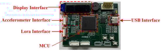
Figure 2.
Computing hardware core of proposed method.
3.2. Dataset Description
To validate the effectiveness of the proposed method, this study uses two datasets for bearing fault diagnosis experiments: one is a bearing fault dataset collected from a self-designed test platform, and the other is a publicly available dataset provided by Paderborn University (PU). The following is a detailed description of these two datasets.
Dataset A: Self-Designed Test Platform Dataset. The dataset is collected from a self-designed bearing fault test platform (Figure 3a), consisting of a motor, coupling, rotor, bearing, and housing, using a 6204 deep groove ball bearing. The signal sampling rate is 10.24 kHz. The platform simulates various bearing fault conditions, including healthy (NF), outer race (OF), inner race (IF), rolling element (RF), and compound (CF) faults, as shown in Figure 4. During testing, the bearing operates at a fixed speed of 800 rpm and 1500 rpm, and vibration signals are collected by an accelerometer mounted on the bearing housing.
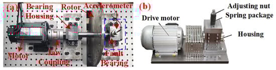
Figure 3.
The main structure of the test platform: (a) the simulation test platform designed by ourselves, and (b) the accelerated life test bench from Paderborn University (PU).
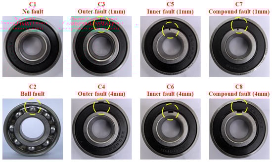
Figure 4.
The bearing fault types: normal bearing (NB), ball fault (BF), outer fault (OF), inner fault (IF), and compound fault (CF).
Dataset B: PU University Dataset. The PU University bearing fault dataset is publicly available and widely used for mechanical fault diagnosis research. It was collected using an accelerated life test apparatus (Figure 3b) with a 64 kHz sampling rate. The dataset includes NF, OF, IF, and CF. Data are gathered under various load, speed, and fault conditions to simulate real-world industrial scenarios (Table 1), and include noise from environmental or equipment vibrations, ensuring diversity and generalizability for cross-domain learning.

Table 1.
Fault types and specifications in the PU dataset.
To be specific, the self-designed test platform dataset simulates bearing faults under controlled conditions with fixed speed and load, and is used for method validation and benchmark testing. The PU dataset, obtained from accelerated life testing, simulates industrial bearing faults with varying loads, speeds, and fault types, offering greater complexity and diversity. By applying the proposed method to both datasets, the robustness and generalization are validated across different operating conditions and fault modes.
3.3. Performance Analysis
To validate the effectiveness of the proposed method, experimental data collected from a simulation test platform are used. As shown in Figure 4, the bearing fault types include NF, BF, IF, OF, and CF, representing five common fault models. Additionally, faults of varying severity levels for IF, OF, and CF are also included to assess the method’s adaptability to different fault severities. Given the limited number of data samples, the original data are divided using a 90% overlap, with each sample containing 10,240 data points. The dataset consists of 600 samples per fault type, totaling 4800 samples for all operating conditions.
Figure 5 shows the time-domain waveforms of different bearing fault modes at 800 rpm. It can be observed that both healthy and rolling element faults lack clear periodic characteristics. This is due to the irregular vibration signals caused by the contact between the rolling elements and the inner and outer races, influenced by the load and contact angle. In particular, early faults produce weak signals that are easily masked by noise, making it difficult for traditional signal analysis methods to detect faults and leading to classification errors in data-driven models. Moreover, as fault severity increases, the amplitude of the waveforms in the OF, IF, and CF changes. Notably, in composite faults, the outer race fault dominates, causing the pulse features to resemble those of the outer race fault, which may lead to misclassification.
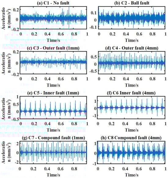
Figure 5.
Time-domain waveform of bearing fault signals from the self-designed test platform.
To address this, the S-transform is introduced to enhance frequency-domain feature extraction and improve signal separability. As shown in Figure 6, the S-transform combines the local properties of short-time Fourier transform (STFT) with the multi-resolution features of wavelet transform, providing detailed time-frequency information to capture signal variations. As a comparison, the Continuous Wavelet Transform (CWT) and STFT are presented in Figure 7 and Figure 8, respectively. Superior than CWT and STFT, the frequency spectrum generated by the S-transform effectively reduces noise interference, highlighting useful frequency-domain features and making different fault types easier to distinguish, thereby improving diagnostic accuracy. Additionally, compared to time-domain signals, the frequency spectrum from the S-transform is more compact, reducing data storage requirements for online deployment, which is suitable for embedded systems and edge computing devices.
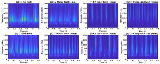
Figure 6.
Time-frequency results of bearing fault after applying the S-transform.
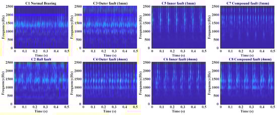
Figure 7.
Time-frequency results of bearing fault after applying the CWT.
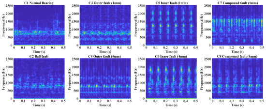
Figure 8.
Time-frequency results of bearing fault after applying the STFT.
Table 2 presents the composition of the source domain and target domain datasets used to validate the model’s effectiveness. To balance diagnostic performance and computational cost, features obtained from the S-transform are uniformly rescaled into RGB images. These image datasets are then randomly split into training and testing sets. The pixel mean of the training set is subtracted to remove irrelevant image information, enhancing the reliability of feature extraction. Additionally, 200 of the training set images are randomly designated as a validation set for dynamic model parameter adjustment.
Table 2.
Detailed information of the source and target datasets.
To further evaluate the diagnostic performance of the proposed framework, a comparison is made with six MobileNet-based diagnostic methods, tested on both time-domain and time-frequency domain datasets. Each method is tested five times on eight fault types, with 200 test samples per fault type. The average accuracy of the experimental results is shown in Table 3. The comparative analysis is as follows:
Table 3.
Diagnostic accuracy under different diagnostic strategies.
- Advantage of Time-Frequency Domain Data: Comparing Method 1 and Method 2, the average accuracy for time-frequency domain data increased by 2.8% (from 85.7% to 88.5%). This indicates that time-frequency data contain richer fault feature information, helping the model better capture fault patterns. Similarly, Method 4 (time-frequency domain) is 2.4% higher than Method 3 (time-domain), and Method 6 (time-frequency domain) is 3.4% higher than Method 5 (time-domain). The advantage of time-frequency data is more prominent in complex tasks.
- Effect of Distillation: Comparing Method 1 and Method 3, distillation improved the average accuracy of the time-domain data by 2.6% (from 85.7% to 88.3%). Similarly, comparing Method 2 and Method 4, distillation improved the average accuracy of the time-frequency domain data by 2.2% (from 88.5% to 90.7%). Distillation enhances the model’s generalization ability through knowledge transfer and regularization.
- Effect of Domain Adaptation: Comparing Method 3 and Method 5, domain adaptation increased the average accuracy for time-domain data by 1.8% (from 88.3% to 90.1%). Similarly, comparing Method 4 and Method 6, domain adaptation improved the average accuracy for time-frequency domain data by 2.8% (from 90.7% to 93.5%). Domain adaptation effectively mitigates the data distribution mismatch, especially for time-frequency data.
- Cumulative Effect of Method Combinations: The proposed method (Method 6) achieved the highest average accuracy of 93.5%, outperforming the baseline Method 1 by 7.8%. The combined effect of these techniques shows that distillation and domain adaptation synergistically maximize model performance when applied to time-frequency domain data.
- Generalization Capability: To evaluate the generalization ability, the proposed method was tested on two datasets: Dataset A (Self-Designed Test Platform Dataset) and Dataset B (PU University Dataset), achieving 93.5% and 94.2% accuracy, respectively. This consistency across datasets with varying operational conditions (e.g., speed, load) demonstrates robustness to domain shifts. Furthermore, we evaluated performance under different noise levels (SNR 0 to 10 dB) and fault severities (1mm to 4mm defects), showing less than 3 % accuracy drop, which underscores its adaptability. Moreover, the integration of domain adaptation further ensures feature invariance across domains.
Therefore, time-frequency domain data are more suitable for fault diagnosis tasks as they provide richer feature information, significantly improving model accuracy. Distillation enhances the model’s generalization ability, especially in data-limited or complex tasks. Domain adaptation effectively addresses data distribution mismatches, particularly in cross-domain diagnostic tasks. The proposed method, with an average accuracy of 93.5% and 94.2% with different datasets, proves to be the optimal approach for bearing fault diagnosis in practical industrial scenarios.
3.4. Comparison with Existing Methods
To evaluate the effectiveness of model compression, Table 4 presents the parameter counts and inference times of both the teacher and student models. The results demonstrate that knowledge distillation significantly reduces model complexity, decreasing the parameter count of the student model from 32.14 k to 8.74 k, a reduction of 72.8%. Concurrently, the inference time is shortened from 20.41 ms to 9.72 ms, a decrease of 52.4%. This indicates that knowledge distillation effectively balances model efficiency with computational performance.
Table 4.
Compression result of the teacher and student model.
To further assess the comprehensive performance of the proposed method, a comparative analysis is conducted against ResNet [] and various lightweight networks, including MobileNet [], ShuffleNet [], GhostNet [], and CGhostNet []. The evaluation metrics encompass diagnostic accuracy, model parameter count, model size, inference time, and computational complexity (FLOPs), as detailed in Table 5.
Table 5.
Comparison of deployment of different models.
The experimental results reveal that ResNet achieves the highest accuracy (98.21%), but it comes with a substantial parameter count of 743.62 k and an inference time of 203.56 ms, resulting in high computational and storage costs, making it unsuitable for real-time or embedded applications. In contrast, the proposed method contains only 8.74k parameters, representing reductions of 98.82%, 72.8%, and 65.8% compared to ResNet, MobileNet, and ShuffleNet, respectively. Although the parameter count is slightly higher than that of CGhostNet (an increase of 4.5%), the accuracy improves to 97.69%, significantly outperforming other lightweight models and approaching the performance of ResNet. Moreover, the inference time is merely 9.91ms, demonstrating superior performance among lightweight architectures and ensuring the feasibility of real-time fault diagnosis.
Additionally, model size is a critical factor for deployment on edge computing devices. GhostNet and CGhostNet exhibit the smallest model sizes (67.5 KB and 46.0 KB, respectively), while the proposed method requires only 51.2 KB—slightly higher than CGhostNet but lower than GhostNet—while achieving significantly higher accuracy (97.69% vs. 85.43% and 87.92%). Therefore, the proposed method demonstrates strong applicability in embedded systems with limited computational resources. To sum up, the proposed method achieves an optimal balance between model size, computational complexity, inference time, and diagnostic accuracy. It maintains high accuracy while significantly reducing computational overhead, demonstrating its effectiveness for real-time fault diagnosis in embedded systems.
3.5. Discussion
Based on the result, it is found that recent advances in model deployment for bearing fault diagnosis emphasize balancing accuracy and efficiency. For instance, quantization-aware training (QAT) and pruning techniques have been widely adopted to compress models for edge deployment. However, these methods often require additional fine-tuning steps to recover accuracy after compression. In contrast, our approach integrates knowledge distillation (KD) from the outset, enabling the student model to inherit the teacher’s discriminative capabilities while reducing parameters by 72.8%. Unlike traditional KD methods that focus solely on logit matching, our framework incorporates feature-level alignment, ensuring the compressed model retains robust feature extraction abilities.
Furthermore, compared to dynamic inference methods, which introduce runtime overhead, our static compressed model achieves real-time inference of 9.72 ms with consistent accuracy across varying loads and speeds. This makes it more suitable for industrial edge devices with fixed computational budgets. The S-transform preprocessing also reduces input dimensionality, further lowering memory usage without sacrificing time-frequency resolution. By prioritizing deployment efficiency, through KD-driven compression and hardware-aware design, our method addresses a critical gap in the field: enabling high-accuracy diagnosis under strict resource constraints.
4. Conclusions
In this paper, we proposed a lightweight fault diagnosis framework that integrates time-frequency analysis, deep learning, and model compression techniques for bearing fault diagnosis in resource-constrained environments. By leveraging the S-transform for high-resolution time-frequency representation and MobileNet as an efficient backbone network, the framework achieves robust fault detection while maintaining computational efficiency. The application of knowledge distillation further compresses the model, enabling real-time deployment on edge devices. Additionally, domain adaptation techniques enhance the model’s generalization across varying operating conditions. Experimental results demonstrate the framework’s effectiveness in achieving high diagnostic accuracy with reduced computational overhead, making it a practical solution for industrial applications.
Nonetheless, it is found that the current work still has limitations, including: (1) Dependency on high-quality vibration signals, which may degrade with sensor placement errors; (2) Limited validation under extreme conditions (e.g., <100 RPM or >3000 RPM); and (3) Computational overhead for very large-scale systems (>1000 bearings). To guide future work, we propose the following: (1) Incorporating active learning to reduce labeling costs, (2) Extending the framework to multi-sensor fusion, such as thermal and acoustic. (3) Optimizing the distillation process for heterogeneous edge devices. These points provide concrete directions for improvement in the future.
Author Contributions
Each author contributed extensively to the preparation of this manuscript. Writing—original draft preparation, X.J.; Investigation, Y.Z.; Writing—review and editing, X.L. and Z.M.; Funding acquisition, F.X. All authors have read and agreed to the published version of the manuscript.
Funding
This work is supported by the National Natural Science Foundation of China under Contract No. 5247514 and No. 52005442, and the Zhejiang Provincial Natural Science Foundation of China under Contract No. LY22E050014.
Institutional Review Board Statement
Not applicable.
Informed Consent Statement
Not applicable.
Data Availability Statement
The original contributions presented in this study are included in the article. Further inquiries can be directed to the corresponding author.
Conflicts of Interest
The authors declare no conflicts of interest.
References
- He, C.; Han, P.; Lu, J.; Wang, X.; Song, J.; Li, Z.; Lu, S. Real-Time Fault Diagnosis of Motor Bearing via Improved Cyclostationary Analysis Implemented onto Edge Computing System. IEEE Trans. Instrum. Meas. 2023, 72, 3524011. [Google Scholar] [CrossRef]
- Ding, A.; Qin, Y.; Wang, B.; Jia, L.; Cheng, X. Lightweight Multiscale Convolutional Networks With Adaptive Pruning for Intelligent Fault Diagnosis of Train Bogie Bearings in Edge Computing Scenarios. IEEE Trans. Instrum. Meas. 2023, 72, 3502813. [Google Scholar] [CrossRef]
- Lu, J.; An, K.; Wang, X.; Song, J.; Xie, F.; Lu, S. Compressed Channel-Based Edge Computing for Online Motor Fault Diagnosis With Privacy Protection. IEEE Trans. Instrum. Meas. 2023, 72, 6505112. [Google Scholar] [CrossRef]
- Li, H.; Hu, G.; Li, J.; Zhou, M. Intelligent Fault Diagnosis for Large-Scale Rotating Machines Using Binarized Deep Neural Networks and Random Forests. IEEE Trans. Autom. Sci. Eng. 2022, 19, 1109–1119. [Google Scholar] [CrossRef]
- Wang, Y.; Wu, J.; Luo, S.; Yu, Z.; Zhou, Q. A Lightweight Reprogramming Framework for Cross-Device Fault Diagnosis in Edge Computing. IEEE Trans. Instrum. Meas. 2025, 74, 3500212. [Google Scholar] [CrossRef]
- Peng, N.; Liang, R.; Wang, G.; Sun, P.; Chen, C.; Hou, T. Edge Computing-Based Fault Location in Distribution Networks by Using Asynchronous Transient Amplitudes at Limited Nodes. IEEE Trans. Smart Grid 2021, 12, 574–588. [Google Scholar] [CrossRef]
- Han, T.; Chao, Z. Fault diagnosis of rolling bearing with uneven data distribution based on continuous wavelet transform and deep convolution generated adversarial network. J. Braz. Soc. Mech. Sci. Eng. 2021, 43, 425. [Google Scholar] [CrossRef]
- Ma, Z.; Fu, L.; Xu, F.; Zhang, L. A physics-based sample generation method for few-shot bearing condition monitoring. Knowl.-Based Syst. 2025, 310, 112952. [Google Scholar] [CrossRef]
- Du, J.; Qin, N.; Huang, D.; Jia, X.; Zhang, Y. Lightweight FL: A Low-Cost Federated Learning Framework for Mechanical Fault Diagnosis With Training Optimization and Model Pruning. IEEE Trans. Instrum. Meas. 2024, 73, 3504014. [Google Scholar] [CrossRef]
- Sun, J.; Liu, Z.; Wen, J.; Fu, R. Multiple hierarchical compression for deep neural network toward intelligent bearing fault diagnosis. Eng. Appl. Artif. Intell. 2022, 116, 105498. [Google Scholar] [CrossRef]
- Huan, L.; Tang, B.; Zhao, C. Global Composite Compression of Deep Neural Network in Wireless Sensor Networks for Edge Intelligent Fault Diagnosis. IEEE Sens. J. 2023, 23, 17968–17978. [Google Scholar] [CrossRef]
- Wang, X.; Hu, D.; Fan, X.; Liu, H.; Yang, C. Intelligent Fault Diagnosis Method Based on Neural Network Compression for Rolling Bearings. Symmetry 2024, 16, 1461. [Google Scholar] [CrossRef]
- Pan, T.; Wang, T.; Chen, J.; Xie, J.; Cao, S. A global and joint knowledge distillation method with gradient-modulated dynamic parameter adaption for EMU bogie bearing fault diagnosis. Measurement 2024, 235, 114927. [Google Scholar] [CrossRef]
- Fu, L.; Yan, K.; Zhang, Y.; Chen, R.; Ma, Z.; Xu, F.; Zhu, T. EdgeCog: A Real-Time Bearing Fault Diagnosis System Based on Lightweight Edge Computing. IEEE Trans. Instrum. Meas. 2023, 72, 2521711. [Google Scholar] [CrossRef]
- Zhang, C.; Qiao, Z.; Li, T.; Kumar, A.; Xu, X.; Li, H.; Li, Z. A teacher-student strategy specific to transformer for machine fault diagnosis. Struct. Health-Monit.-Int. J. 2024. [Google Scholar] [CrossRef]
- An, Y.; Zhang, K.; Chai, Y.; Zhu, Z.; Liu, Q. Gaussian Mixture Variational-Based Transformer Domain Adaptation Fault Diagnosis Method and Its Application in Bearing Fault Diagnosis. IEEE Trans. Ind. Inform. 2024, 20, 615–625. [Google Scholar] [CrossRef]
- Zhang, W.; Li, X.; Ma, H.; Luo, Z.; Li, X. Universal Domain Adaptation in Fault Diagnostics With Hybrid Weighted Deep Adversarial Learning. IEEE Trans. Ind. Inform. 2021, 17, 7957–7967. [Google Scholar] [CrossRef]
- Tang, Z.; Hou, X.; Huang, X.; Wang, X.; Zou, J. Domain Adaptation for Bearing Fault Diagnosis Based on SimAM and Adaptive Weighting Strategy. Sensors 2024, 24, 4251. [Google Scholar] [CrossRef] [PubMed]
- Zhang, H.; Wang, X.; Zhang, C.; Li, W.; Wang, J.; Li, G.; Bai, C. Dynamic Condition Adversarial Adaptation for Fault Diagnosis of Wind Turbine Gearbox. Sensors 2023, 23, 9368. [Google Scholar] [CrossRef]
- Fu, L.; Wang, S.; Chen, R.; Ma, Z.; Ma, J.; Yao, B.; Xu, F. Intelligent Fault Diagnosis of Rolling Bearings Based on an Improved Empirical Wavelet Transform and ResNet Under Variable Conditions. IEEE Sens. J. 2023, 23, 29097–29108. [Google Scholar] [CrossRef]
- Li, G.; Liu, Z.; Zhang, X.; Lin, W. Lightweight Salient Object Detection in Optical Remote-Sensing Images via Semantic Matching and Edge Alignment. IEEE Trans. Geosci. Remote Sens. 2023, 61, 5601111. [Google Scholar] [CrossRef]
- Chen, Z.; Yang, J.; Chen, L.; Jiao, H. Garbage classification system based on improved ShuffleNet v2. Resour. Conserv. Recycl. 2022, 178, 106090. [Google Scholar] [CrossRef]
- Cao, M.; Fu, H.; Zhu, J.; Cai, C. Lightweight tea bud recognition network integrating GhostNet and YOLOv5. Math. Biosci. Eng. 2022, 19, 12897–12914. [Google Scholar] [CrossRef] [PubMed]
- Huang, Q.; Han, Y.; Zhang, X.; Sheng, J.; Zhang, Y.; Xie, H. FFKD-CGhostNet: A Novel Lightweight Network for Fault Diagnosis in Edge Computing Scenarios. IEEE Trans. Instrum. Meas. 2023, 72, 3536410. [Google Scholar] [CrossRef]
Disclaimer/Publisher’s Note: The statements, opinions and data contained in all publications are solely those of the individual author(s) and contributor(s) and not of MDPI and/or the editor(s). MDPI and/or the editor(s) disclaim responsibility for any injury to people or property resulting from any ideas, methods, instructions or products referred to in the content. |
© 2025 by the authors. Licensee MDPI, Basel, Switzerland. This article is an open access article distributed under the terms and conditions of the Creative Commons Attribution (CC BY) license (https://creativecommons.org/licenses/by/4.0/).