Trajectory Tracking Control Strategy of 20-Ton Heavy-Duty AGV Considering Load Transfer

Abstract

During the operation of outdoor heavy-duty Automated Guided Vehicle (AGV), the stability and safety of AGV are easily reduced due to load transfer. In order to solve this problem, a trajectory tracking control strategy considering load transfer is proposed to realize the trajectory tracking of AGV and the adaptive distribution of driving torque. The three-degree-of-freedom (3-DOF) kinematics model and pose error model of heavy-duty AGV vehicles are established. The lateral load transfer and longitudinal load transfer rules are analyzed. The vehicle trajectory tracking control strategy is composed of an improved model predictive controller (IMPC) and drive motor torque adaptive distribution controller considering load transfer. By optimizing the lateral acceleration of the vehicle body, the IMPC controller improves the problem of large driving force difference between the left and right sides of the wheel caused by the lateral transfer of the load and the problem of large wheel adhesion rate caused by the longitudinal transfer of the load is improved by the speed controller and the torque proportional distribution controller. The joint simulation platform of MATLAB/Simulink and CarSim is built to simulate and analyze the trajectory tracking of heavy-duty AGV under different pavement adhesion coefficients. The simulation results have shown that compared with the control strategy without considering load transfer, on the two types of pavements with different adhesion coefficients, the maximum lateral acceleration is reduced by 19.7%, and the maximum tire adhesion rate is reduced by 11.5%.

1. Introduction

With the proposal of the Made in China 2025 plan, the intelligence level of China’s manufacturing industry is constantly improving, and the degree of unmanned is getting higher and higher. Automatic Guided Vehicle (AGV) is generally composed of a mechanical structure, power unit, and control system. It can travel autonomously according to the route specified by the dispatching system and avoid obstacles automatically [1]. At present, AGV is widely used in logistics warehousing [2], manufacturing [3], port terminals [4], aircraft assembly [5], and other fields, which greatly improves production efficiency and industrial competitiveness.

The application and research of AGV mostly focus on structural design and optimization [6], path planning [7], trajectory tracking [8], and scheduling [9] of light-load and small-size AGV. Using reasonable control methods to achieve trajectory tracking is one of the important tasks of AGV operation. The commonly used trajectory tracking control methods are classical proportional-integral-derivative (PID) control [10], MPC [11], sliding mode control (SMC) [12], H∞ robust control [13], fuzzy intelligent control method [14], and the combination of two or more different control methods, such as fuzzy PID control [15], adaptive sliding mode control [16], etc. Wu et al. [17] proposed a new backstepping and fuzzy sliding mode controller for differential wheeled mobile robots. Based on the kinematic model, the backstepping kinematic controller is established. Based on the dynamic model, the integer order integral sliding mode controller is established. At the same time, the fuzzy controller is used to estimate and compensate for the disturbance, which has a good control effect. Zhang et al. [18] proposed an adaptive learning model predictive control scheme. Based on the AGV kinematics model, the estimated system parameters are used in the MPC to improve the prediction accuracy. Yildiz et al. [19] designed a robust, non-chattering sliding mode control method for linear following robots and carried out numerical solutions and experimental research. Compared with the traditional PID control method, the sliding mode controller has higher path-tracking efficiency. Han et al. [20] proposed a new dynamic coefficient reaching law to speed up the response speed of the sliding mode control system and designed a double closed-loop control to realize the trajectory tracking of the automatic guided vehicle. Wang et al. [21] proposed a robust model predictive control strategy to realize the trajectory tracking of omnidirectional AGV under different constraints and applied the delayed neural network (DNN) to solve the quadratic programming (QP) problem. Compared with the traditional neural network, the computational complexity is reduced, and the online solution speed is improved. The robustness and effectiveness of the proposed method are verified by simulation analysis. Xing et al. [22] proposed a robust nonsingular terminal sliding mode (NTSM) control method based on a recurrent neural network (RNN) structure to improve the trajectory tracking performance of AGV. The robustness and effectiveness of the proposed control method for parameter uncertainties and unknown external disturbances are verified by simulation. Liu et al. [23] designed an adaptive sliding mode dynamic controller based on disturbance observer, which realized the online estimation of disturbance and completely eliminated the chattering phenomenon. The effectiveness of the proposed scheme is verified by simulation. Chen et al. [24] proposed an adaptive neural network control scheme for uncertain wheeled mobile robots with speed constraints and nonholonomic constraints. For the uncertainty of the robot, the adaptive neural network is used to approximate the unknown robot dynamics and the barrier Lyapunov function is used to guarantee the constraint on velocity. The effectiveness of the proposed control scheme is proved by simulation research and practical experiments. Most of the above research is to improve tracking accuracy for the purpose of control algorithm design.

The transportation of heavy parts has high labor intensity, high safety risk, and low workpiece transfer efficiency. It is urgent to improve the level of intelligence and unmanned, which is of great significance for the research of heavy-duty AGVs [25]. Compared with light-load AGV, heavy-load AGV has a larger load and higher center of gravity. More stability problems need to be considered in the design of control methods, and the control system is more complex. In order to improve the handling stability of electric vehicles, Liu et al. [26] designed a three-layer control strategy to improve the driving stability of the vehicle body by controlling the yaw rate and centroid sideslip angle of the vehicle body. The effectiveness of the proposed control strategy is verified by simulation and experiment. Fu et al. [27] used the centroid sideslip angle as an index to evaluate the rollover behavior of AGV and used the multi-body dynamics simulation model to analyze the influence of turning rate, center of mass height, and pavement adhesion coefficient on the rollover stability of heavy-duty AGV. Aiming at the stability and safety problems caused by the failure of the actuator, Zhang et al. [28] designed a top-level optimal input controller based on MPC theory, a middle-level expected yaw moment solver based on fuzzy theory, and a bottom-level torque reconfiguration control distributor based on control gain. The hierarchical controller, and through simulation and experiment, proves that the yaw rate and the centroid sideslip angle of the center of mass can track the theoretical value well, and the designed controller is effective. Aiming at the problem that the centroid of AGV changes due to the irregular position and uneven weight of goods on the cargo on the load platform, Liu et al. [29] proposed a hierarchical control strategy to improve yaw stability considering centroid variation, which reduced the yaw rate and centroid sideslip angle of AGV. Most of the above studies have improved the stability of heavy-duty AGVs by reducing the yaw rate and centroid sideslip angle of the center of mass during heavy-duty AGV driving. However, due to the large difference in the driving force required by the left and right wheels during heavy-duty AGV driving caused by load transfer and the unreasonable distribution of the driving force required by the front and rear wheels, the problem of large adhesion rate has not been considered.

The above research optimizes different control methods for various application scenarios of heavy-duty AGVs to meet their special operational requirements. The heavy-duty AGV studied in this paper has the characteristic of large inertia. During driving in outdoor industrial areas, significant lateral and longitudinal load transfers are prone to occur during starting, braking, turning, or encountering potholes, speed bumps, and other conditions. For the vehicle body, lateral load transfer causes uneven wheel loads on both sides, leading to changes in the friction between the AGV wheels and the road surface. The power of the drive motor in this paper is almost equally distributed to the two side wheels through the differential, which can cause excessive torque on the inner wheels and insufficient torque on the outer wheels. Increasing the motor torque output may lead to inner wheel slippage or drive motor overload. Longitudinal load transfer changes the vertical loads on the front and rear wheels. When one wheel has a low load and high driving torque, wheel slippage may occur due to a high wheel adhesion rate. Therefore, both lateral and longitudinal load transfers have adverse effects on vehicle driving stability. To reduce these adverse effects while considering tracking accuracy, this paper designs a control strategy for heavy-duty low-speed AGVs with double Ackermann steering. The proposed strategy combines an improved MPC controller that restricts lateral load transfer, a PID vehicle speed controller, and a torque proportional distribution controller. Compared with the conventional MPC controller, the improved MPC controller enhances the prediction model and objective function design. The prediction model not only forecasts the AGV’s pose error but also considers the prediction output of the load transfer evaluation index. Additionally, an objective function is designed to minimize the load transfer amount, tracking error, and control increment. Finally, a co-simulation platform using MATLAB/Simulink R2021a and CarSim 2020.0 is built to verify the rationality and feasibility of the proposed control strategy.

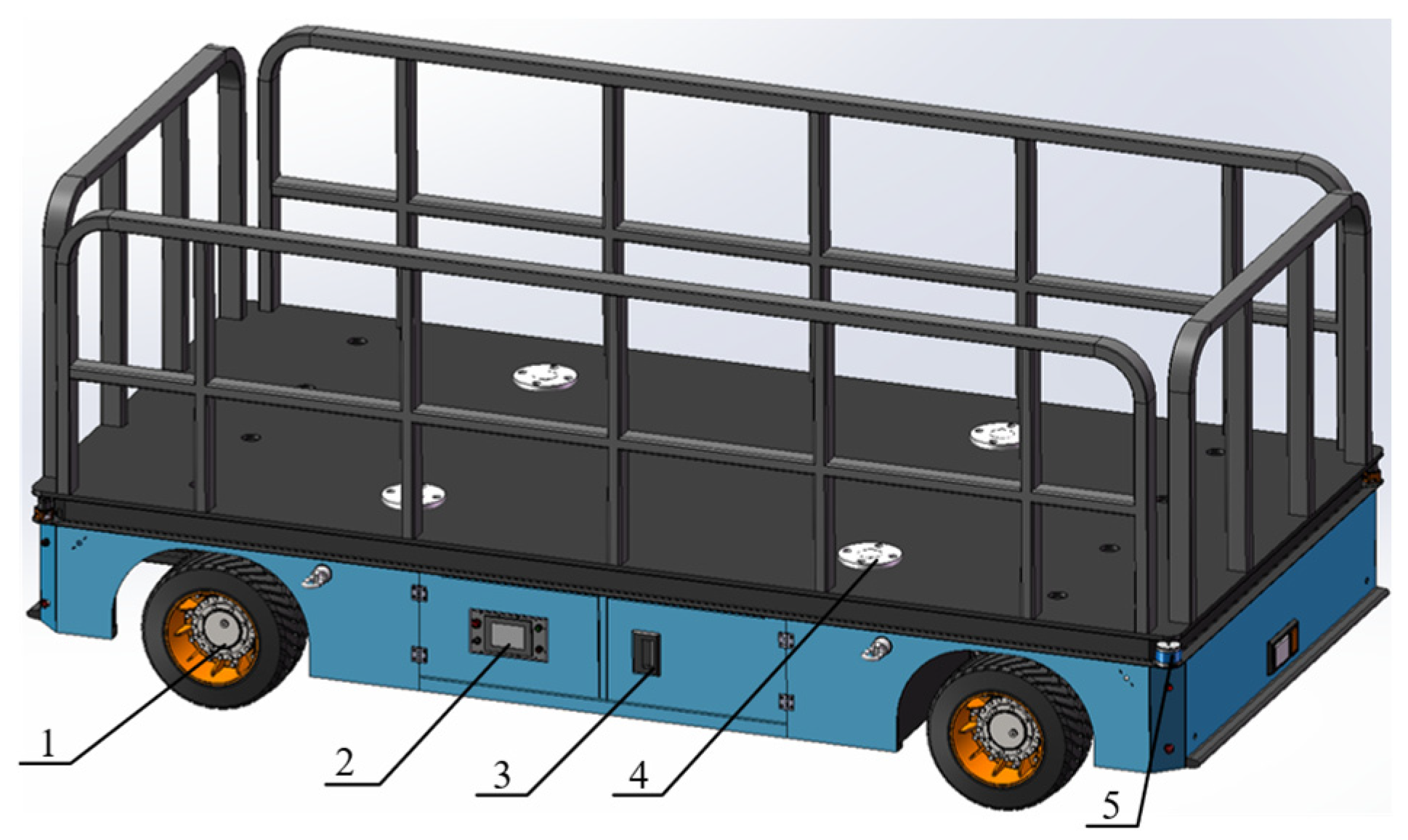
2. Establishment of Heavy-Duty AGV Vehicle Model

The 20-ton heavy-duty AGV studied in this paper mainly includes the drive module, lifting module, power module, control module, laser radar, and other parts. It is used for intelligent unmanned transportation of liquid ton buckets and small buckets in the factory area. When running, there are both curves and ramps with a maximum slope of 10%. When the liquid in the bucket turns, the load transfer to the outside of the curve occurs. When driving on the ramp, it moves back and forth to make the load difference between the front and rear axles large. Both load transfers affect the stability and safety of the vehicle. The driving module is used to drive the vehicle movement, the lifting module is used to lift the goods, the control module is used to control the vehicle to perform various expected actions, such as trajectory tracking and lifting actions, and the lidar is used to detect the operating environment and map construction. The three-dimensional model of the heavy-duty AGV is shown in Figure 1.

Common vehicle models mainly include three-degree-of-freedom (3-DOF) bicycle models, as well as five-degree-of-freedom and seven-degree-of-freedom four-wheeler models. The bicycle model is suitable for analyzing the basic handling stability of the vehicle, and the four-wheeler model is suitable for analyzing the dynamic response of the vehicle under high-speed driving and complex pavement conditions. The motion process of heavy-duty AGVs is highly nonlinear. Although the more complex the vehicle model is, the closer the analysis results are to the real motion law, the calculation amount is greatly increased, which reduces the timeliness of the controller. The heavy-duty AGVs running in the factory have low speed and large inertia. The three-degree-of-freedom vehicle model can meet the research needs of this paper while reducing the amount of calculation. Therefore, this paper establishes a three-degree-of-freedom vehicle kinematics model and a linear error model.

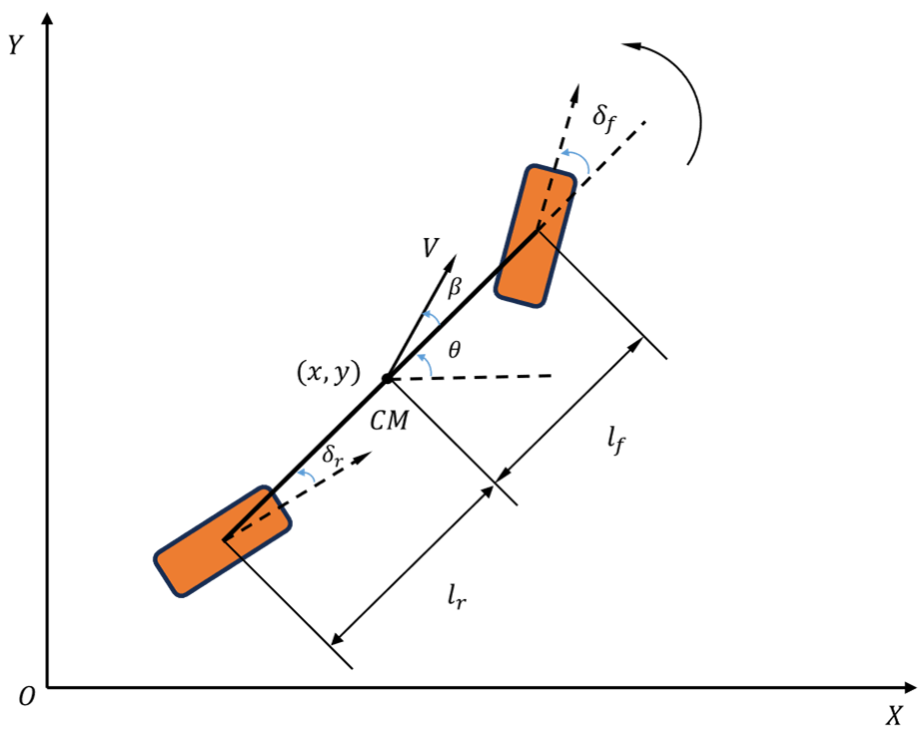
2.1. Three-Degree-of-Freedom Vehicle Kinematics Model

The steering modes of heavy-duty AGV mainly include four-wheel independent drive, four-wheel independent steer (4WID/4WIS) type [30], differential wheel type [31], Mecanum wheel type [32], single Ackerman steering type [33], and double Ackerman steering type. Although the 4WID/4WIS is flexible and changeable, the cost of the 4WID/4WIS is high, and the requirements for the motor and control accuracy are high. The differential wheel steering structure is relatively simple, and the cost is relatively low, but the requirements for ground flatness are harsh, and the load is light. Mecanum wheel steering is more flexible and can achieve movement in all directions, but the ground flatness requirements are higher, and the price is high; although the structure of the single Ackerman steering is simple, the flexibility is poor because there is only one steering shaft. Double Ackerman steering has higher flexibility, a smaller steering radius, and better driving stability, which is suitable for complex environments with changeable pavements. To sum up, the heavy-duty AGV designed in this paper is used in the scene where the outdoor factory pavement is changeable and has certain flexibility and stability requirements, so the double Ackerman steering is selected. A front and rear dual-motor drive configuration is adopted, with permanent magnet synchronous motors selected as the drive motors. Considering the operating conditions and design requirements of the heavy-duty AGV during operation, the power of a single-drive motor is calculated. The finally selected motor has a rated power of 75 kW, a rated torque of 477 N∙m, and a rated speed of 1500 r/min.

The double Ackerman steering geometric model is shown in Figure 2. It mainly includes the front and rear wheels and the steering center, in which the steering wheels on both sides are connected by the steering axle. When the model is established, the main parameters considered are the front and rear left and right wheel angles δ_fl, δ_fr, δ_rl, δ_rr, which are simplified to the equivalent front and rear wheel angles δ_f, δ_r; wheel track W; wheelbase l; the longitudinal distance l₁ and l₂ from the steering center to the front and rear axles; and the vertical distance R from the steering center to the center of the car body. CE is the steering center of AGV.

From Figure 2, the relationship between the rotation angles δ_fl, δ_fr, δ_rl, δ_rr of each wheel and the rotation angles δ_f, δ_r of the front and rear wheels after cycling can be obtained as follows:

$${\delta }_{fl}=\arctan {\displaystyle \frac{2l_1}{2R-W}}$$

(1)

$${\delta }_{fr}=\arctan {\displaystyle \frac{2l_1}{2R+W}}$$

(2)

$${\delta }_{rf}=\arctan {\displaystyle \frac{-2l_2}{2R-W}}$$

(3)

$${\delta }_{rr}=\arctan {\displaystyle \frac{-2l_2}{2R+W}}$$

(4)

where $R={\displaystyle \frac{l_1}{\tan {\delta }_f}}$, $l_1={\displaystyle \frac{l\cdot \tan {\delta }_f}{\tan {\delta }_f-\tan {\delta }_r}}$, $l_2={\displaystyle \frac{-l\cdot \tan {\delta }_r}{\tan {\delta }_f-\tan {\delta }_r}}$

The relationship between δ_f and δ_r is

$${\displaystyle \frac{\tan {\delta }_f}{\tan {\delta }_r}}={\displaystyle \frac{l_1}{l_1-l}}$$

(5)

From (1)~(4), the relationship between the steering wheel angles on both sides can be obtained:

$$\cot {\delta }_{fr}-\cot {\delta }_{fl}={\displaystyle \frac{W}{l_1}}$$

(6)

$$\cot {\delta }_{rf}-\cot {\delta }_{rr}={\displaystyle \frac{W}{l_2}}$$

(7)

From (6) and (7), it can be seen that when the wheel track W is determined, the size of l₁ and l₂ is related to the wheel rotation angle δ_fl, δ_fr, δ_rl, and δ_rr. The wheels on both sides are connected by the steering bridge. Taking the front wheel as an example, the relationship between δ_fl and δ_fr is related to the geometric parameters of the steering trapezoid in the front steering bridge. When the steering trapezoid parameters are determined, the relationship between δ_fl and δ_fr can be determined. When W is constant, the size of l₁ can be determined, and so is the rear wheel.

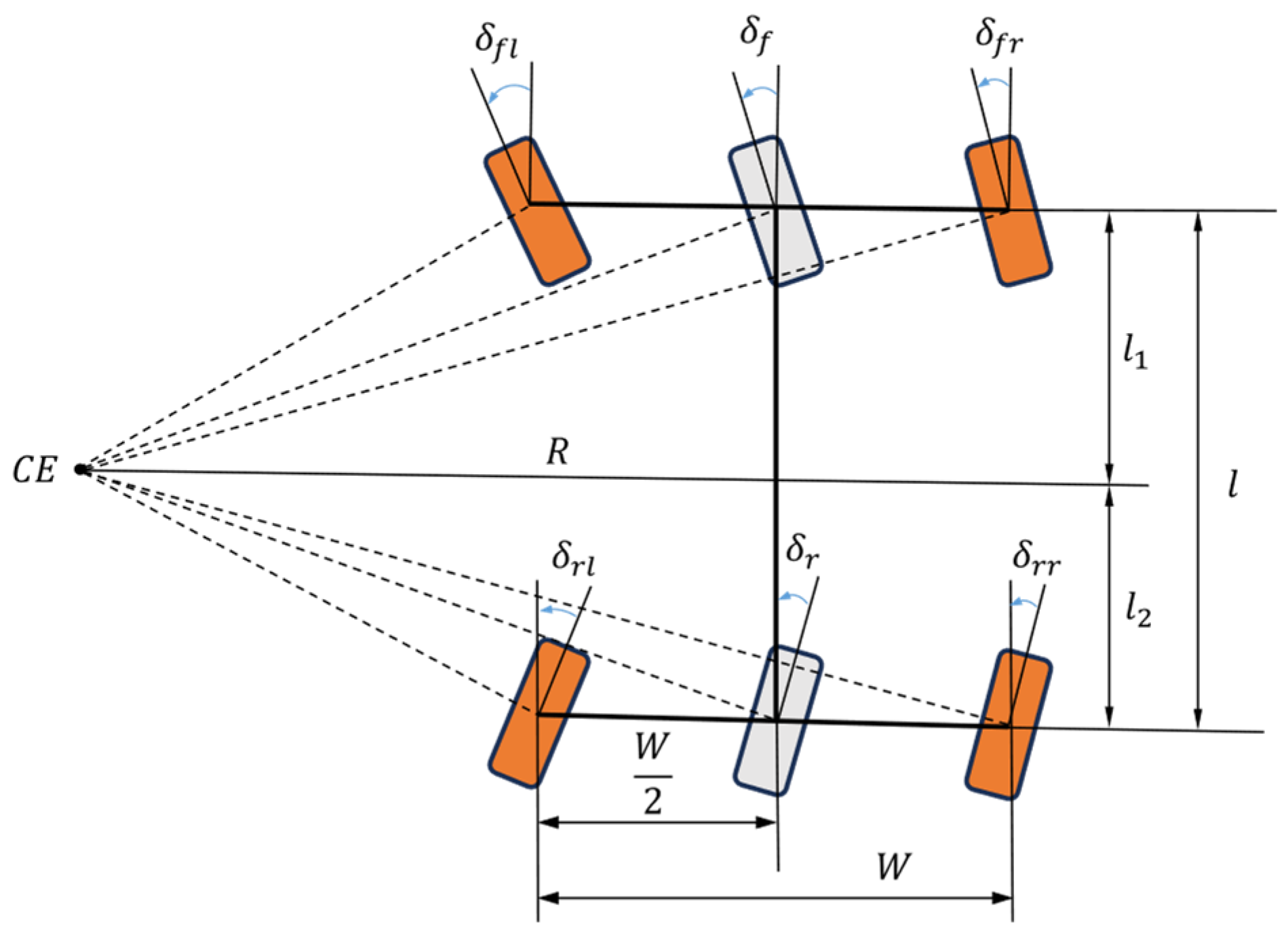
2.2. Pose Linear Error Model of Double Ackermann Steering

By establishing a pose linear error model, the deviation between the current state of the AGV and the desired trajectory can be described more accurately so that the prediction model can be easily established when designing the model predictive control. In order to reduce the complexity of the model and improve the solution speed, the motion model of the double Ackerman steering heavy-duty AGV is simplified into a bicycle model, as shown in Figure 3.

XOY is the geodetic coordinate system. CM is the centroid of AGV, and its coordinate is (x, y). V is the centroid velocity. β is the centroid sideslip angle of AGV’s mass center. θ is the angle between the AGV longitudinal and the horizontal axis of the coordinate system. l_f and l_r are the longitudinal distances from the center of mass of AGV to the center of the front wheel and rear wheel, respectively, and l_f = l_r = 1.5 m.

It can be obtained from Figure 3:

$$\tan \beta ={\displaystyle \frac{l_r\tan {\delta }_f+l_f\tan {\delta }_r}{l_f+l_r}}$$

(8)

The load of AGV is large. When the centroid sideslip angle of the center of mass is large, it is easy to cause problems such as reduced stability of the vehicle and increased tire wear. Therefore, it is necessary to reduce the centroid sideslip angle of the center of mass to reduce the above effects. It can be obtained from (8) that when l_f = l_r, in order to make the theoretical centroid sideslip angle of the center of mass zero, it is necessary to satisfy

$${\delta }_r=-{\delta }_f$$

(9)

When δ_r = −δ_f, l₁ = l/2 can be obtained from (5), so the parameters of the steering trapezoid in the front and rear steering transmission mechanism of AGV, as shown in Figure 4, can be determined by (6) and (7).

The motion state model of AGV is shown in (10):

$$.\left[\begin{array}{c}\dot{x}\\ \dot{y}\\ \dot{\theta }\end{array}\right]=\left[\begin{array}{c}v\cdot \cos (\beta +\theta )\\ v\cdot \sin (\beta +\theta )\\ v\cdot \cos (\beta ){\displaystyle \frac{\tan {\delta }_f-\tan {\delta }_r}{l_f+l_r}}\end{array}\right].$$

(10)

where $(\dot{x},\dot{y},\dot{\theta })$ is the derivative of AGV pose $(x,y,\theta )$ at different moments.

$X={[x,y,\theta ]}^T$ and $u={[{\delta }_f,{\delta }_r,v]}^T$ are selected as the state variable and input control variable of AGV, respectively. The (10) can be expressed as

$$\dot{X}=f(X,u)$$

(11)

For a given reference trajectory, it can be described by the motion trajectory of the reference vehicle. Each point on it satisfies the above motion state equation, and r represents the reference variable. The general form is

$${\dot{X}}_r=f(X_r,u_r)$$

(12)

where $X_r={[x_r,y_r,{\theta }_r]}^T$, $u_r={[{\delta }_{fr},{\delta }_{rr},v_r]}^T$.

Expanding (11) at the reference point $(x_r,y_r,{\theta }_r)$ using a Taylor series and neglecting higher-order terms, the following expression can be obtained:

$$\dot{X}=f(X_r,u_r)+{\displaystyle \frac{\partial f(X,u)}{\partial X}}(X-X_r)+{\displaystyle \frac{\partial f(X,u)}{\partial u}}(u-u_r)$$

(13)

The linear time-varying error model of the AGV pose obtained by subtracting (12) and (13) is as follows:

$${\dot{X}}_e=\dot{X}-{\dot{X}}_r=\left[\begin{array}{c}\dot{x}-{\dot{x}}_r\\ \dot{y}-{\dot{y}}_r\\ \dot{\theta }-{\dot{\theta }}_r\end{array}\right]=A_t{X}_e+B_t{u}_e$$

(14)

where $A_t=\left[\begin{array}{ccc}0& 0& -v_r\sin \left({\theta }_r\right)\\ 0& 0& v_r\cos \left({\theta }_r\right)\\ 0& 0& 0\end{array}\right]$, $X_e={\left[x-x_r,y-y_r,\theta -{\theta }_r\right]}^T$, $u_e={\left[{\delta }_f-{\delta }_{fr},{\delta }_r-{\delta }_{rr},v-v_r\right]}^T$, $B_t=\left[\begin{array}{ccc}{\displaystyle \frac{-v_r\sin \left({\theta }_r\right)\left(1+{\tan }^2{\delta }_{fr}\right)}{2}}& {\displaystyle \frac{-v_r\sin \left({\theta }_r\right)\left(1+{\tan }^2{\delta }_{fr}\right)}{2}}& \cos \left({\theta }_r\right)\\ {\displaystyle \frac{v_r\cos \left({\theta }_r\right)\left(1+{\tan }^2{\delta }_{fr}\right)}{2}}& {\displaystyle \frac{v_r\cos \left({\theta }_r\right)\left(1+{\tan }^2{\delta }_{fr}\right)}{2}}& \sin \left({\theta }_r\right)\\ {\displaystyle \frac{v_r\left(1+{\tan }^2{\delta }_{fr}\right)}{l_f+l_r}}& -{\displaystyle \frac{v_r\left(1+{\tan }^2{\delta }_{rr}\right)}{l_f+l_r}}& {\displaystyle \frac{\tan {\delta }_{fr}-\tan {\delta }_{rr}}{l_f+l_r}}\end{array}\right]$.

In Equation (14), the reference pose (x_r, y_r, θ_r) and the reference input (δ_fr, δ_rr, v_r) vary with time, l_f = l_r = 1.5 m. Therefore, the values of A_t and B_t vary with time, but at a certain time, A_t and B_t are known, and Equation (14) is linear. In order to simplify the calculation process and apply the obtained pose linear error model to the model predictive controller, the (14) needs to be discretized to establish the prediction model of the trajectory tracking error, and the prediction model is used to predict the future system state. Based on these predictions, the control action is optimized to make more accurate and effective decisions.

3. Load Transfer Analysis

When the heavy-duty AGV runs in a uniform straight line on a flat pavement, the vertical loads borne by the four wheels of the vehicle are basically the same. When turning, or when there are pits, speed bumps, or a certain slope on the pavement, the load borne by the vehicle is transferred to a certain extent, and the load distribution borne by the vehicle body changes so that the vertical load borne by each wheel changes. Load transfer is divided into lateral load transfer and longitudinal load transfer.

3.1. Lateral Load Transfer Analysis

When turning, the AGV’s own load and cargo load transfers from the inner wheel to the outer wheel; that is, the lateral load transfer occurs. When the vehicle speed is large, the lateral load transfer is easy to cause the vehicle to roll over [34]. The heavy-duty AGV travels at a small speed and has a large load. Although the load transfer effect does not cause the vehicle to roll over, it causes uneven wheel load on both sides, resulting in changes in the friction between the AGV wheel and the pavement surface. In this paper, the power of the drive motor is almost evenly distributed to the wheels on both sides through the differential, which easily causes the torque of the inner wheel to be too large and the torque of the outer wheel to be insufficient. If the torque output of the motor is increased, it may cause the inner wheel to slip, or the drive motor is overloaded, which reduces the service life of the wheel. In order to avoid large lateral load transfer during vehicle motion, it is necessary to design a controller to optimize the relevant variables.

The vertical load acting on the wheel is equal to the vertical reaction force acting on the wheel by the ground. The lateral load transfer can be determined by analyzing the vertical reaction force acting on the AGV wheel by the ground. In order to facilitate the analysis of the vertical reaction force of the left and right wheels, the AGV is simplified to the model shown in Figure 5. The I-shaped frame shown in Figure 5a is supported by elastic elements on the front and rear axles, where G_s is the total gravity of AGV and cargo, P_f and P_r are the roll centers of front and rear suspensions. Figure 5b shows the lateral force distribution of the frame. The centrifugal force F_ay acting on the carriage is distributed to the roll center P_f and P_r of the front and rear suspensions according to the position of the vehicle center of mass, which is balanced by the lateral reaction forces F_syf and F_syr at the front and rear roll centers. Figure 5c,d are shown as the force diagram of the front and rear axles. In the analysis, the total gravity of the AGV and the cargo in the static state is separated from the vertical reaction force of the ground on the corresponding four wheels as an equilibrium force system.

In Figure 5b, F_syf and F_syr are the lateral reaction forces of the front and rear suspensions to balance the centrifugal force F_ay. The following can be obtained:

$$F_{syf}=F_{ay}{\displaystyle \frac{l_r}{l_r+l_f}}$$

(15)

$$F_{syr}=F_{ay}{\displaystyle \frac{l_f}{l_r+l_f}}$$

(16)

The torque of the front and rear suspensions relative to the front and rear roll centers is

$$T_{ff}=K_{ff}{f}_r$$

(17)

$$T_{fr}=K_{fr}{f}_r$$

(18)

where K_ϕ and K_ϕr are the roll angle stiffness of the front and rear suspensions, and ϕ_r is the frame roll angle.

In Figure 5c,d, the variation in the vertical reaction force of the left and right wheels can be obtained by taking the moment balance at the touch point of each wheel:

$$\Delta F_{zfl}W=F_{ay}{\displaystyle \frac{l_r}{l_f+l_r}}{h}_f+T_{ff}+F_{ufy}{h}_{uf}$$

(19)

$$\Delta F_{zfr}W=-F_{ay}{\displaystyle \frac{l_r}{l_f+l_r}}{h}_f-T_{ff}-F_{ufy}{h}_{uf}$$

(20)

$$\Delta F_{zrl}W=F_{ay}{\displaystyle \frac{l_f}{l_f+l_r}}{h}_r+T_{fr}+F_{ury}{h}_{ur}$$

(21)

$$\Delta F_{zrr}W=-F_{ay}{\displaystyle \frac{l_f}{l_f+l_r}}{h}_r-T_{fr}-F_{ury}{h}_{ur}$$

(22)

where ∆F_zfl, ∆F_zfr, ∆F_zrl, and ∆F_zrr are the variations in the vertical reaction forces of the left and right wheels of the front and rear axles; F_ufy and F_ury are the lateral forces generated by the non-suspended mass of the front and rear axles; h_uf and h_ur are the height from the ground of the mass center of the non-suspended mass; h_f and h_r are the height of the center of mass of the front and rear axles.

From the (19)~(22), it can be seen that the variation in the vertical reaction force of the wheel is related to the centrifugal force F_ay; the centroid height h_f, h_r of the front and rear axles; the front and rear suspension roll torque T_ϕf, T_ϕr; the lateral force F_ufy, F_ury generated by the unsuspended mass; and the off-ground height h_uf, h_ur of the unsuspended mass centroid. Compared with the load of AGV, the unsuspended mass is smaller, and the lateral force caused by the unsuspended mass is ignored. T_ϕf and T_ϕr are related to the roll angle and roll angle stiffness of the suspension, and it is difficult to adjust. Therefore, the load transfer can be reduced by optimizing F_ay. Because F_ay = ma_y and the total mass m of AGV is large, a_y must be optimized. The lateral acceleration of the centroid can be expressed as

$$a_y={\dot{v}}_y+v_x\dot{\theta }$$

(23)

where ${\dot{v}}_y=\dot{v}\sin (\beta )$, $v_x\dot{\theta }=v^2{\cos }^2\beta {\displaystyle \frac{\tan {\delta }_f-\tan {\delta }_r}{l_f+l_r}}$.

When the centroid sideslip angle β is zero,

$$a_y=v^2{\displaystyle \frac{\tan {\delta }_f-\tan {\delta }_r}{l_f+l_r}}$$

(24)

In order to reduce the lateral load transfer of heavy-duty AGV and improve the driving stability, it is necessary to optimize the lateral acceleration a_y.

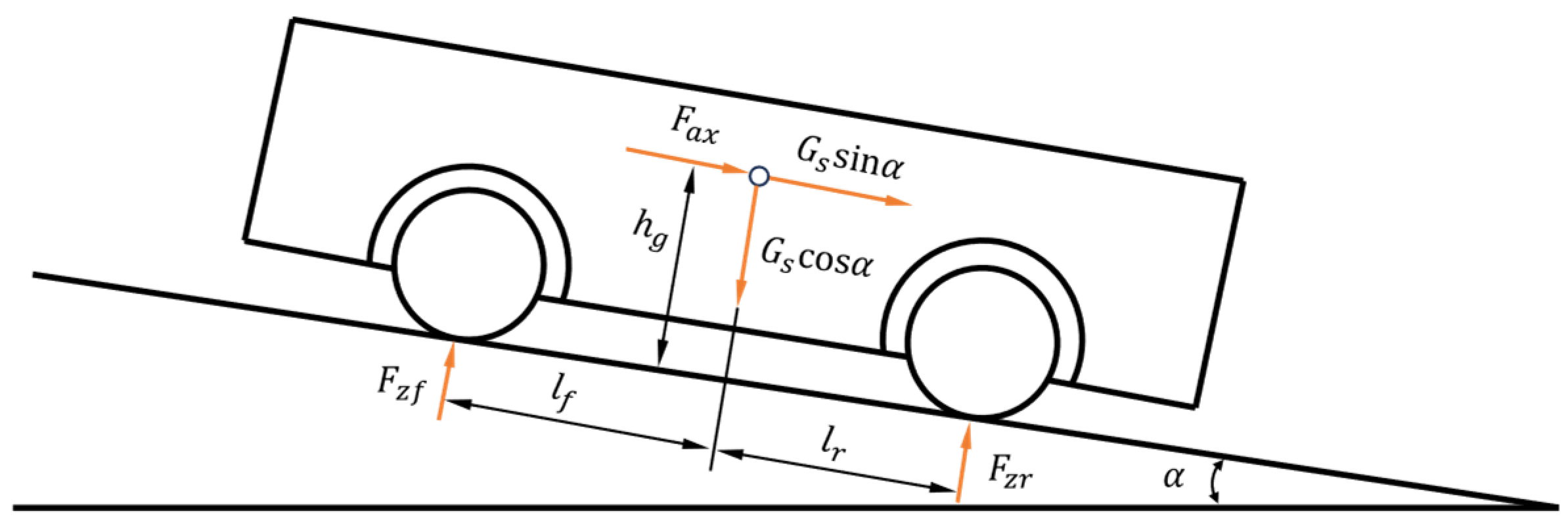
3.2. Longitudinal Load Transfer Analysis

When the vehicle starts, brakes, runs on a ramp or accelerates or decelerates in a straight line, or when there are pits and speed bumps on the pavement surface, under the action of inertial force, the load on the vehicle is transferred before and after, that is, the longitudinal load transfer, which causes the vertical load of the front and rear wheels to change, ranging in size (does not cause the load of the left and right wheels to vary). When the wheel load on one side is low, and the driving torque is large, the wheel slips due to the high wheel adhesion rate. In order to avoid this phenomenon, it is necessary to design a torque distribution controller to redistribute the driving torque of the front and rear motors.

The longitudinal load transfer can be determined by analyzing the vertical reaction force acting on the AGV wheel on the ground. In order to facilitate the analysis of the vertical reaction force of the front and rear wheels, the rotational inertia resistance moment and the rolling resistance moment are ignored. Due to the low speed, the air lift is ignored. When analyzing the longitudinal load transfer, the heavy-duty AGV is simplified to the model shown in Figure 6. In the figure, Gs is the total gravity of the vehicle, α is the slope angle of the pavement, h_g is the centroid height of the vehicle, l_f and l_r are the distances from the front axle and the rear axle to the center of mass of the vehicle, l is the wheelbase of the vehicle, F_zf and F_zr are the normal reaction forces acting on the front and rear wheels of the vehicle.

The torque of each force acting on the vehicle to the center of the contact surface between the front and rear wheels and the pavement can be obtained:

$$F_{zf}=G_s({\displaystyle \frac{l_f}{l_f+l_r}}\cos \alpha -{\displaystyle \frac{h_g}{l_f+l_r}}\sin \alpha )-F_{ax}{\displaystyle \frac{h_g}{l_f+l_r}}$$

(25)

$$F_{zr}=G_s({\displaystyle \frac{l_r}{l_f+l_r}}\cos \alpha +{\displaystyle \frac{h_g}{l_f+l_r}}\sin \alpha )+F_{ax}{\displaystyle \frac{h_g}{l_f+l_r}}$$

(26)

The normal reaction force acting on each wheel can be obtained by the simultaneous (18)~(21), (25) and (26):

$$F_{zfl}={\displaystyle \frac{G_s}{2}}({\displaystyle \frac{l_f}{l_f+l_r}}\cos \alpha -{\displaystyle \frac{h_g}{l_f+l_r}}\sin \alpha )-{\displaystyle \frac{F_{ax}}{2}}{\displaystyle \frac{h_g}{l_f+l_r}}+\Delta F_{zfl}$$

(27)

$$F_{zfr}={\displaystyle \frac{G_s}{2}}({\displaystyle \frac{l_f}{l_f+l_r}}\cos \alpha -{\displaystyle \frac{h_g}{l_f+l_r}}\sin \alpha )-{\displaystyle \frac{F_{ax}}{2}}{\displaystyle \frac{h_g}{l_f+l_r}}+\Delta F_{zfr}$$

(28)

$$F_{zrl}={\displaystyle \frac{G_s}{2}}({\displaystyle \frac{l_r}{l_f+l_r}}\cos \alpha +{\displaystyle \frac{h_g}{l_f+l_r}}\sin \alpha )+{\displaystyle \frac{F_{ax}}{2}}{\displaystyle \frac{h_g}{l_f+l_r}}+\Delta F_{zrl}$$

(29)

$$F_{zrr}={\displaystyle \frac{G_s}{2}}({\displaystyle \frac{l_r}{l_f+l_r}}\cos \alpha +{\displaystyle \frac{h_g}{l_f+l_r}}\sin \alpha )+{\displaystyle \frac{F_{ax}}{2}}{\displaystyle \frac{h_g}{l_f+l_r}}+\Delta F_{zrr}$$

(30)

From (27)~(30), it can be seen that the normal reaction force on each wheel is related to the parameters such as the vertical reaction force variation in the wheel ∆F_zfl, ∆F_zfr, ∆F_zrl, ∆F_zrr; the total gravity of the vehicle G_s; the slope angle of the pavement α; and the centroid height of the vehicle h_g, and has a high nonlinear relationship with the slope angle of the pavement α. Based on the vertical load of each wheel calculated by Formulas (27)~(30), the subsequent torque distribution control strategy can be designed.

4. Design of Trajectory Tracking Control Strategy Considering Load Transfer

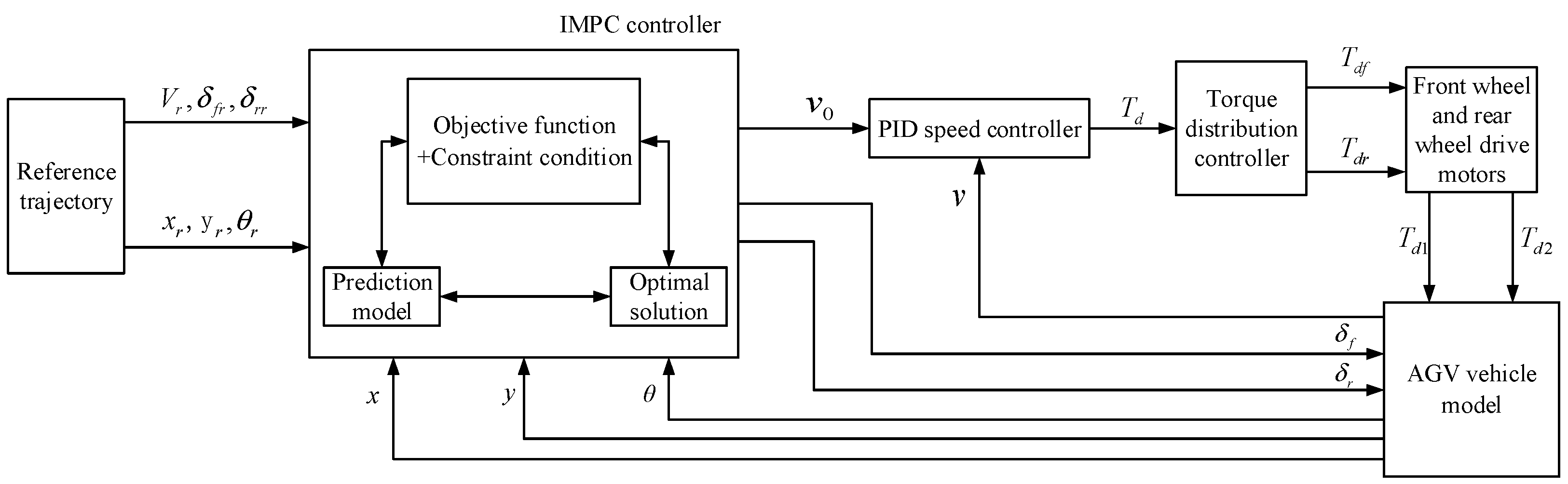
4.1. Overall Control Strategy Design

Aiming at the phenomenon of load transfer caused by turning driving, pavement slope, acceleration and deceleration, or pits and deceleration zones on the pavement during the operation of heavy-duty AGV, this paper proposes a heavy-duty AGV trajectory tracking control strategy considering load transfer. The lateral load transfer control adopts an IMPC controller considering lateral acceleration optimization, and the longitudinal load transfer control adopts a driving torque proportional distribution controller. The structure of the control system is shown in Figure 7.

The control system shown in Figure 7 consists of three parts:

• An MPC controller for optimizing lateral acceleration based on the kinematic model. The improved MPC controller receives the state reference quantities (x_r, y_r, θ_r) output by the reference trajectory, the control reference quantities (v_r, δ_fr, δ_rr), and the actual pose (x, y, θ) of the AGV. A cost function that minimizes both the lateral acceleration term and the tracking error term is designed, along with constraints on the maximum and minimum values of the control variables and their increments, as well as the equality constraint in Equation (9). A prediction model is established to output the control variables and perform feedback correction so as to achieve AGV trajectory tracking while reducing the lateral load transfer;
• A velocity controller for calculating the total driving torque. The PID velocity controller receives the desired velocity v₀ output by the MPC controller and the actual velocity v of the AGV, thereby computing and outputting the total driving torque T_d of the AGV;
• A torque distribution controller for allocating the total driving torque to each motor and transferring it to the vehicle model. After receiving the total driving torque calculated by the PID velocity controller, the torque distribution controller allocates the total driving torque into the input torques T_df and T_dr of the front and rear drive motors according to the vertical load proportion allocation method, thereby driving the AGV movement.

4.2. Lateral Load Transfer IMPC Control Strategy

The conventional PID controller should have limited external interference ability, complex parameter adjustment, and experience dependence when performing trajectory tracking control, and it is difficult to deal with multivariate and constraint problems. The MPC controller can effectively solve the above problems. By continuously establishing the prediction model and designing the objective function, the optimal input control variables of each step are obtained, which act on the controlled object. It has the advantages of strong robustness and convenient consideration of the constraints of the controlled system. When the conventional MPC controller is used for trajectory tracking control, the established prediction model only predicts the pose error information of AGV, and the designed objective function only aims at the minimum tracking error and control increment. In this paper, the conventional MPC controller is improved. When designing the prediction model, the evaluation variables of load transfer are considered to predict the output, and the objective function with the minimum load transfer, tracking error, and control increment is designed.

4.2.1. Design of Prediction Model

When designing the prediction model, it is necessary to consider which variables will predict the output. At present, most of the MPC controllers used in trajectory tracking control only consider predicting the tracking error and ignore the influence of load transfer when designing the prediction model. In this paper, the following improvements are made: the lateral acceleration a_y is optimized to reduce the lateral load transfer. In (24), the rotation angle is assumed to be a small angle, δ_f − δ_r is used to approximately replace tanδ_f − tanδ_r, and the speed v and the difference between the front and rear rotation angles δ_f − δ_r are predicted to improve the tracking accuracy of AGV. The adverse effects of load transfer on the vehicle are reduced.

In order to apply the linear error model obtained from (14) to the design of the model predictive controller, the forward Euler method is used to discretize Equation (14), and the state space equation of the discrete system is obtained, as shown in Equation (31).

$$X_e(k+1)=a_k{X}_e(k)+b_k{u}_e(k)$$

(31)

where k is a moment, T is the sampling period, $a_k=\left[\begin{array}{ccc}1& 0& -T{v}_r\sin ({\theta }_r)\\ 0& 1& T{v}_r\cos ({\theta }_r)\\ 0& 0& 1\end{array}\right]$, $b_k=\left[\begin{array}{ccc}{\displaystyle \frac{-T{v}_r\sin ({\theta }_r)(1+{\tan }^2{\delta }_{fr})}{2}}& {\displaystyle \frac{-T{v}_r\sin ({\theta }_r)(1+{\tan }^2{\delta }_{fr})}{2}}& T\cos ({\theta }_r)\\ {\displaystyle \frac{T{v}_r\cos ({\theta }_r)(1+{\tan }^2{\delta }_{fr})}{2}}& {\displaystyle \frac{T{v}_r\cos ({\theta }_r)(1+{\tan }^2{\delta }_{fr})}{2}}& T\sin ({\theta }_r)\\ {\displaystyle \frac{T{v}_r(1+{\tan }^2{\delta }_{fr})}{l_f+l_r}}& -{\displaystyle \frac{T{v}_r(1+{\tan }^2{\delta }_{rr})}{l_f+l_r}}& {\displaystyle \frac{T(\tan {\delta }_{fr}-\tan {\delta }_{rr})}{l_f+l_r}}\end{array}\right].$

To facilitate the constraint of the control increment and optimize the influencing factors v and δ_f − δ_r of the lateral acceleration in the objective function, a new state variable ξ(k) is constructed by combining X_e(k) and u_e(k − 1); that is, $\xi (k)={[X_e\left(k),u_e\right(k-1\left)\right]}^T$. Then, by introducing the coefficient C, the required output variable η(k) is obtained as η(k) = ${\left[x\right(k)-x_r(k),y\left(k)-y_r\right(k),\theta \left(k\right)-{\theta }_r(k),\left({\delta }_f(k-1)-{\delta }_{\mathit{fr}}(k-1)\right)-({\delta }_r(k-1)-{\delta }_{\mathit{rr}}(k-1)\left),v\right(k-1)-v_r(k-1\left)\right]}^T$. The first three items represent the longitudinal, lateral, and yaw angle errors, respectively, and the last two items are related to the lateral acceleration. The state–space expression is

$$\left\{\begin{array}{c}\xi (k+1)=A_k\xi (k)+B_k\Delta u(k)\\ \eta (k)=C\xi (k)\end{array}\right.$$

(32)

where $A_k=\left[\begin{array}{cc}{a}_k& b_k\\ 0_{N_u\times N_x}& I_{N_u}\end{array}\right]$, $B_k=\left[\begin{array}{c}{b}_k\\ I_{N_u}\end{array}\right]$, $C=\left[\begin{array}{cc}{I}_{N_x}& 0_{N_x\times N_u}\\ 0_{1\times N_x}& c_{\delta }\\ 0_{1\times N_x}& c_v\end{array}\right]$, $c_{\delta }=\left[1,-1,0\right]$, $c_v=\left[0,0,1\right]$.

The future horizon of the system is N_p, the control horizon is N_c, and the predictive output of each step in the predictive time domain is

$$Y=\Psi \xi (k)+\Theta \Delta U$$

(33)

where $Y={\left[\begin{array}{cccccc}\eta \left(k+1\right)& \eta \left(k+2\right)& \cdots & \eta \left(k+N_c\right)& \cdots & \eta \left(k+N_p\right)\end{array}\right]}^T$, $\Psi ={\left[\begin{array}{cccccc}C{A}_k& C{A_k}^2& \cdots & C{A_k}^{N_c}& \cdots & C{A_k}^{N_p}\end{array}\right]}^T$, $\Delta U={\left[\begin{array}{cccc}\Delta u\left(k\right)& \Delta u\left(k+1\right)& \cdots & \Delta u\left(k+N_c-1\right)\end{array}\right]}^T$, $\Theta =\left[\begin{array}{cccc}C{B}_k& 0& 0& 0\\ C{A}_k{B}_k& C{B}_k& 0& 0\\ \cdots & \cdots & \ddots & \cdots \\ C{A_k}^{N_c-1}{B}_k& C{A_k}^{N_c-2}{B}_k& \cdots & C{B}_k\\ C{A_k}^{N_c}{B}_k& C{A_k}^{N_c-1}{B}_k& \cdots & C{A}_k{B}_k\\ ⋮& ⋮& \ddots & ⋮\\ C{A_k}^{N_p-1}{B}_k& C{A_k}^{N_p-2}{B}_k& \cdots & C{A_k}^{N_p-N_c-1}{B}_k\end{array}\right]$.

It can be seen from (33) that the output variable in the future horizon can be calculated by the state variable ξ(k) at the current time and the control increment ∆U in the control horizon.

4.2.2. Design of Objective Function

The objective function should be able to ensure that the AGV tracks the desired trajectory quickly and smoothly while considering the load transfer. Therefore, the following objective function is established with the objective of minimizing the deviation of system state variables, lateral load transfer, and control increment:

$$J={(Y-Y_r+F)}^T{Q}_w(Y-Y_r+F)+\Delta U^T{R}_w\Delta U+\rho {\epsilon }^2$$

(34)

where Q_w and R_w are weight matrices, $Q_w={\left[\begin{array}{cccc}{q}_w& 0& \cdots & 0\\ 0& q_w& \cdots & 0\\ ⋮& ⋮& \ddots & ⋮\\ 0& 0& 0& q_w\end{array}\right]}_{N_p\times N_p}$, $R_w={\left[\begin{array}{cccc}{r}_w& 0& \cdots & 0\\ 0& r_w& \cdots & 0\\ ⋮& ⋮& \ddots & ⋮\\ 0& 0& 0& r_w\end{array}\right]}_{N_c\times N_c}$, $q_w=\left[\begin{array}{ccccc}20& 0& 0& 0& 0\\ 0& 20& 0& 0& 0\\ 0& 0& 20& 0& 0\\ 0& 0& 0& 0.3& 0\\ 0& 0& 0& 0& 10\end{array}\right]$, $r_w=\left[\begin{array}{ccc}10& 0& 0\\ 0& 10& 0\\ 0& 0& 10\end{array}\right]$, $Y_r={\left[\begin{array}{ccccc}0& \cdots & 0& \cdots & 0\end{array}\right]}^T$, $F_g={\left[\begin{array}{cccccc}{f}_g\left(k\right)& f_g\left(k+1\right)& \cdots & f_g\left(k+N_c-1\right)& \cdots & f_g\left(k+N_p-1\right)\end{array}\right]}^T$, $f_g\left(k\right)=\left[\begin{array}{c}{0}_{N_x\times 1}\\ {\delta }_{fr}\left(k\right)-{\delta }_{rr}\left(k\right)\\ v_r\left(k\right)\end{array}\right]$.

The first term in (34) reflects the ability of the system to track the reference trajectory and the optimization of the lateral acceleration. The second term reflects the stability of the change in the input control variables of the system. The third term is a relaxation factor term introduced to ensure that each optimization goal has a feasible solution, where ρ is the weight of the relaxation factor, and ε is the relaxation factor.

Substituting (33) into (34) can obtain

$$J=E^T{Q}_{w}E+\Delta U^T({\Theta }^T{Q}_w\Theta +R_w)\Delta U+2E^T{Q}_w\Theta \Delta U+\rho {\epsilon }^2$$

(35)

where $E=\Psi \xi \left(k\right)+F_g$, $E^T{Q}_{w}E$ is a constant, which can be discarded in the solution.

Further processing of (35) to convert it into a QP problem:

$$\underset{\Delta U}{\min }J={\displaystyle \frac{1}{2}}\Delta V^{T}H\Delta V+G^T\Delta V$$

(36)

where $\Delta V=\left[\begin{array}{cc}\Delta U& \epsilon \end{array}\right]$, $H=\left[\begin{array}{cc}{\Theta }^T{Q}_w{\Theta }^T+R_w& 0\\ 0& \rho \end{array}\right]$, $G^T=\left[\begin{array}{cc}{E}^T{Q}_w\Theta & 0\end{array}\right]$.

4.2.3. Constraint Condition Design Based on Double Ackerman Angle Constraint

In order to avoid the drastic change in control input and maintain the stability of the system, it is necessary to set the maximum and minimum constraints on the input control variable U_e and the control increment ∆U and set the equality constraint of δ_f = −δ_r for the front and rear corners according to the (9). The relationship between the input control variable U_e and the control increment ΔU can be obtained by derivation:

$$\begin{array}{ll}{U}_e& =\left[\begin{array}{c}{u}_e(k)\\ u_e(k+1)\\ ⋮\\ u_e(k+N_c-1)\end{array}\right]=\left[\begin{array}{c}{u}_e(k-1)\\ u_e(k-1)\\ ⋮\\ u_e(k-1)\end{array}\right]+\left[\begin{array}{ccccc}{I}_{N_c}& 0& 0& \cdots & 0\\ I_{N_c}& I_{N_c}& 0& \cdots & 0\\ ⋮& ⋮& ⋮& \ddots & ⋮\\ I_{N_c}& I_{N_c}& I_{N_c}& \cdots & I_{N_c}\end{array}\right]\left[\begin{array}{c}\Delta u(k)\\ \Delta u(k+1)\\ \Delta u(k+2)\\ ⋮\\ \Delta u(k+N_c-1)\end{array}\right]\\ & =U_t+A_I\Delta U\end{array}$$

(37)

Therefore, the inequality constraint of control increment can be obtained:

$$\left\{\begin{array}{c}{A}_I\Delta U\le U_{\max }-U_t\\ -A_I\Delta U\le -U_{\min }+U_t\\ \Delta U\le \Delta U_{\max }\\ \Delta U\ge \Delta U_{\min }\end{array}\right.$$

(38)

where U_t is the actual input control variable at time k − 1, U_max and U_min are the maximum and minimum values of the input control variable U_e, ∆U_max and ∆U_min are the maximum and minimum values of the control increment.

From (9), δ_f = −δ_r can be obtained, and equality constraints need to be added. From (37), we can obtain

$$\begin{array}{ll}U& =\left[\begin{array}{c}u(k)\\ u(k+1)\\ ⋮\\ u(k+N_c-1)\end{array}\right]=\left[\begin{array}{c}{u}_e(k-1)+u_r(k)\\ u_e(k-1)+u_r(k+1)\\ ⋮\\ u_e(k-1)+u_r(k+N_c+1)\end{array}\right]+\left[\begin{array}{ccccc}{I}_{N_c}& 0& 0& \cdots & 0\\ I_{N_c}& I_{N_c}& 0& \cdots & 0\\ ⋮& ⋮& ⋮& \ddots & ⋮\\ I_{N_c}& I_{N_c}& I_{N_c}& \cdots & I_{N_c}\end{array}\right]\left[\begin{array}{c}\Delta u(k)\\ \Delta u(k+1)\\ \Delta u(k+2)\\ ⋮\\ \Delta u(k+N_c-1)\end{array}\right]\\ & =U_t+U_r+A_I\Delta U\end{array}$$

(39)

Therefore, the following formulas can be obtained:

$$Eq=\left[\begin{array}{c}{\delta }_f(k)+{\delta }_r(k)\\ {\delta }_f(k+1)+{\delta }_r(k+1)\\ ⋮\\ {\delta }_f(k+N_c-1)+{\delta }_r(k+N_c-1)\end{array}\right]=\left[\begin{array}{cccc}\kappa & 0& \cdots & 0\\ 0& \kappa & \cdots & 0\\ ⋮& ⋮& \ddots & ⋮\\ 0& 0& 0& \kappa \end{array}\right]U={\rm K}(U_t+U_r+A_I\Delta U)$$

(40)

where κ = [1, 1, 0], U_r is the reference value of rotation angle and velocity at different moments.

Thus, the equality constraint of control increment can be obtained:

$$Eq=0$$

(41)

So far, the optimization problem of model predictive control can be transformed into a standard QP problem:

$$\left\{\begin{array}{c}\underset{\Delta U}{\min }J={\displaystyle \frac{1}{2}}\Delta V^{T}H\Delta V+G\Delta V\\ \mathrm{s}.\mathrm{t}.\left\{\begin{array}{c}\begin{array}{c}{A}_I\Delta U_t\le U_{\max }-U_t\\ -A_I\Delta U_t\le -U_{\min }+U_t\\ \Delta U\le \Delta U_{\max }\\ \Delta U\ge \Delta U_{\min }\end{array}\\ Eq=0\end{array}\right.\end{array}\right.$$

(42)

In each control cycle, a series of control increment ∆U values can be obtained by solving the Equation (42). In order to improve the accuracy of the prediction, only the first result of the obtained control sequence is used as input to the system, and the same operation is performed at the next moment; the cycle is repeated until the trajectory tracking is completed.

4.3. Torque Adaptive Distribution Longitudinal Load Transfer Control Strategy

The longitudinal load transfer control strategy of torque adaptive distribution is composed of a PID speed controller and torque distribution controller. The PID speed controller realizes the tracking of the speed output by the improved MPC controller, and the output is the total driving torque T_d of the vehicle. The total driving torque is distributed to the front and rear motors through the torque distribution module and finally acts on the dynamic model of the vehicle. The structure diagram of the longitudinal load transfer control strategy with adaptive torque distribution is shown in Figure 8.

The driving torque T_d formula calculated by the PID speed controller at time t is:

$$T_d=K_{P}e(t)+K_I{\displaystyle \int e(t)dt}+K_D{\displaystyle \frac{de(t)}{dt}}$$

(43)

$$e(t)=V_0(t)-V(t)$$

(44)

where V₀(t) is the expected speed of MPC output at time t; V(t) is the actual speed of the vehicle at time t; K_p, K_I, and K_D are the proportional coefficient, integral coefficient, and differential coefficient, respectively, and their specific values of 10,000, 8000, and 0.1 are obtained through continuous trial and adjustment during the simulation process; and e(t) is the difference between the expected speed and the actual speed at time t.

In order to adapt to the situation of load transfer before and after AGV operation, it is necessary to adaptively allocate the driving torque to prevent the wheel adhesion rate on one side from being large due to the unequal vertical load on the front and rear wheels, thus reducing the driving stability of AGV. The commonly used methods of torque distribution controller include the average distribution method [35], the proportional distribution method according to the vertical load of the wheel [36], and the quadratic programming method with the goal of economy or stability [37]. In this paper, the proportional distribution method of the vertical load of the wheel is used to distribute the torque based on the vertical load of each wheel calculated by (27) to (30).

$$T_{df}={\displaystyle \frac{F_{Zfl}+F_{zfr}}{F_{Zfl}+F_{zfr}+F_{Zrl}+F_{zrr}}}{T}_d$$

(45)

$$T_{dr}={\displaystyle \frac{F_{zrl}+F_{zrr}}{F_{zfl}+F_{zfr}+F_{Zrl}+F_{zrr}}}{T}_d$$

(46)

In order to prevent the driving force of the vehicle from exceeding the pavement adhesion limit, the maximum driving torque constraint of the front and rear wheels is set as follows:

$$T_{df}\le \mu \min (F_{zfl},F_{zfr})$$

(47)

$$T_{dr}\le \mu \min (F_{zrl},F_{zrr})$$

(48)

where μ is the pavement adhesion coefficient.

At this point, the design of the trajectory tracking control strategy for heavy-duty AGV considering load transfer is completed. The IMPC controller is used for lateral load transfer control. The improvements are in the design of the prediction model and objective function. By predicting the related items of pose error and acceleration, the objective function, which considers tracking error and lateral load transfer, is designed. The longitudinal load transfer control adopts the driving torque proportional distribution controller.

5. Trajectory Tracking Co-Simulation Analysis Based on Simulink and CarSim

The above-mentioned heavy-duty AGV runs on both curves and ramps with a maximum slope of 10%. When the established vehicle model is relatively simple, it is impossible to truly restore the AGV operation, and it is difficult to solve the vehicle model when it is complex. Therefore, the numerical simulation cannot test the effect of the control strategy well, while CarSim can easily and accurately modify the vehicle, pavement surface, and other information; establish an accurate vehicle dynamics model; and facilitate joint simulation with MATLAB/Simulink. In this paper, the AGV model was established in CarSim, and then the controller was designed in Simulink. Based on MATLAB/Simulink and CarSim, the joint simulation of heavy-duty AGV trajectory tracking is carried out.

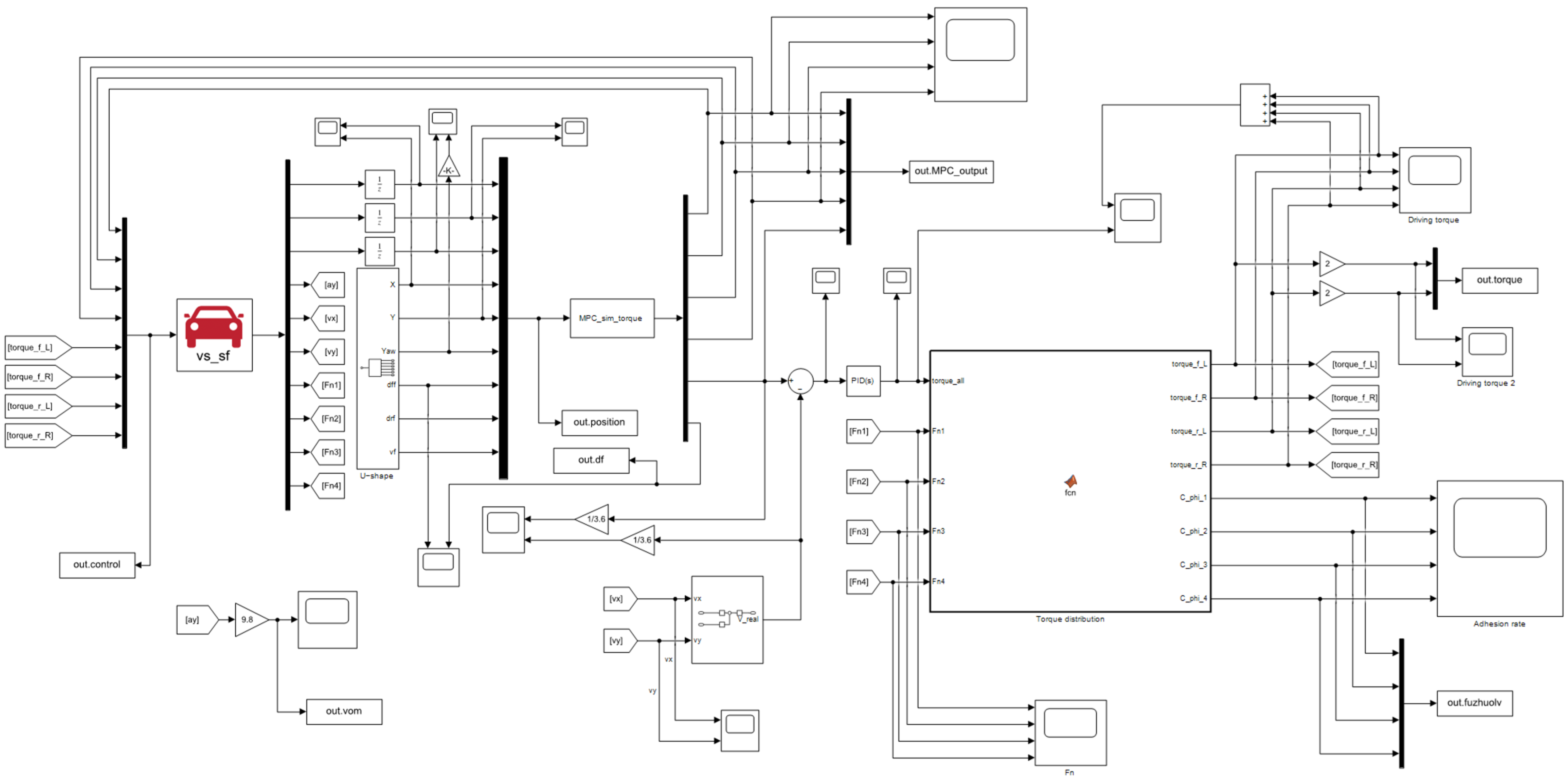
5.1. Establishment of a Simulation Model

The basic parameters of the heavy-duty AGV are shown in

Table 1. Basic parameters of heavy-duty AGV.

Parameter	Unit	Value
Overall size (length/width/height)	m	5/2.4/0.6
wheelbase	m	3
wheel track	m	2.1
dead weight	t	5
load	t	20
reference speed	m/s	0.5

.

After setting the various parameters of AGV, as shown in Table 1 in CarSim, it is imported into Simulink, and a joint simulation model of the control strategy is established in Simulink, as shown in Figure 9.

Figure 9 demonstrates the following:

• The IMPC controller receives the state reference quantities (x_r, y_r, θ_r) output by the reference trajectory, the control reference quantities (v_r, δ_fr, δ_rr), and the actual pose (x, y, θ) of the AGV from CarSim. By solving the constrained objective function described above, the front and rear wheel angles and the desired velocity are calculated;
• The PID velocity controller computes and outputs the total driving torque T_d of the AGV based on the error between the actual velocity and the desired velocity;
• The torque distribution controller receives the total driving torque T_d calculated by the PID velocity controller and allocates it into the driving torques T_df and T_dr of the front and rear drive motors according to the vertical load proportion allocation method, which is then output to the CarSim module;
• The CarSim module receives the front and rear wheel driving torques from the torque distribution controller and the front and rear wheel angles from the IMPC controller to control the vehicle’s driving and steering and feeds back the vehicle’s state information.

In order to effectively test the effect of the control strategy designed above, a U-shaped reference trajectory is constructed as the AGV driving trajectory for simulation analysis. The reference trajectory consists of five paths, including flat pavement, turning, and slope pavement, where l_p1, l_p2, l_p3, and l_p4 are straight flat pavements; l_p1 and l_p2 are connected by a semi-circular flat pavement with a radius of 8 m; and l_p3 is a straight slope with a slope of 10%. The length of each path is shown in Figure 10. The designed reference path covers straight driving, turning driving, and slope driving, which can test the effect of the control strategy.

Because the adhesion conditions of the outdoor pavement in the factory area are affected by various factors, the adhesion coefficient varies greatly. Therefore, two kinds of pavements with different adhesion coefficients are set up for simulation analysis, and the control effects under five different control strategies are analyzed. Different control strategies are shown in

Table 2. Different control strategies.

Name	Trajectory Tracking Method	Torque Distribution Method
PID-TED	PID	Torque Equal Distribution
MPC-TED	MPC	Torque Equal Distribution
IMPC-TED	IMPC	Torque Equal Distribution
MPC-TPD	MPC	Torque Proportional Distribution
IMPC-TPD	IMPC	Torque Proportional Distribution
PID-TED	PID	Torque Equal Distribution

.

The speed controllers of the five different control strategies are all PID speed controllers, and the difference lies in the trajectory tracking method and the torque distribution method. As shown in Table 2, PID-TED control adopts the control strategy combining the PID controller and Torque Equal Distribution (TED) controller. MPC-TED control adopts the control strategy combining the MPC controller and TED controller. IMPC-TED control adopts the control strategy combining IMPC controller and TED controller. The MPC-TPD control adopts the control strategy of combining the MPC controller with the torque proportional distribution (TPD) controller, and the IMPC-TPD control adopts the control strategy of combining the IMPC controller with the TPD controller.

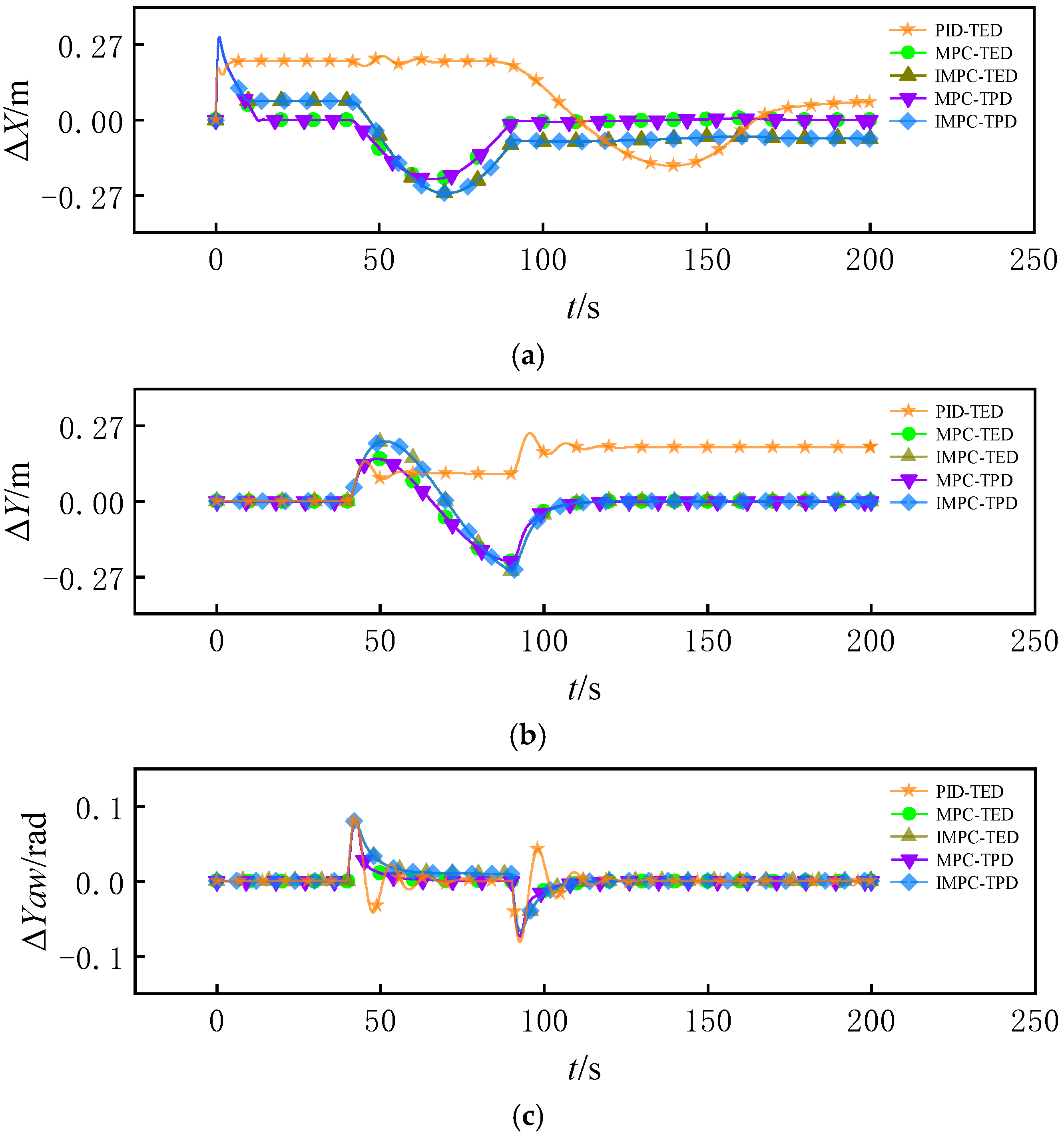
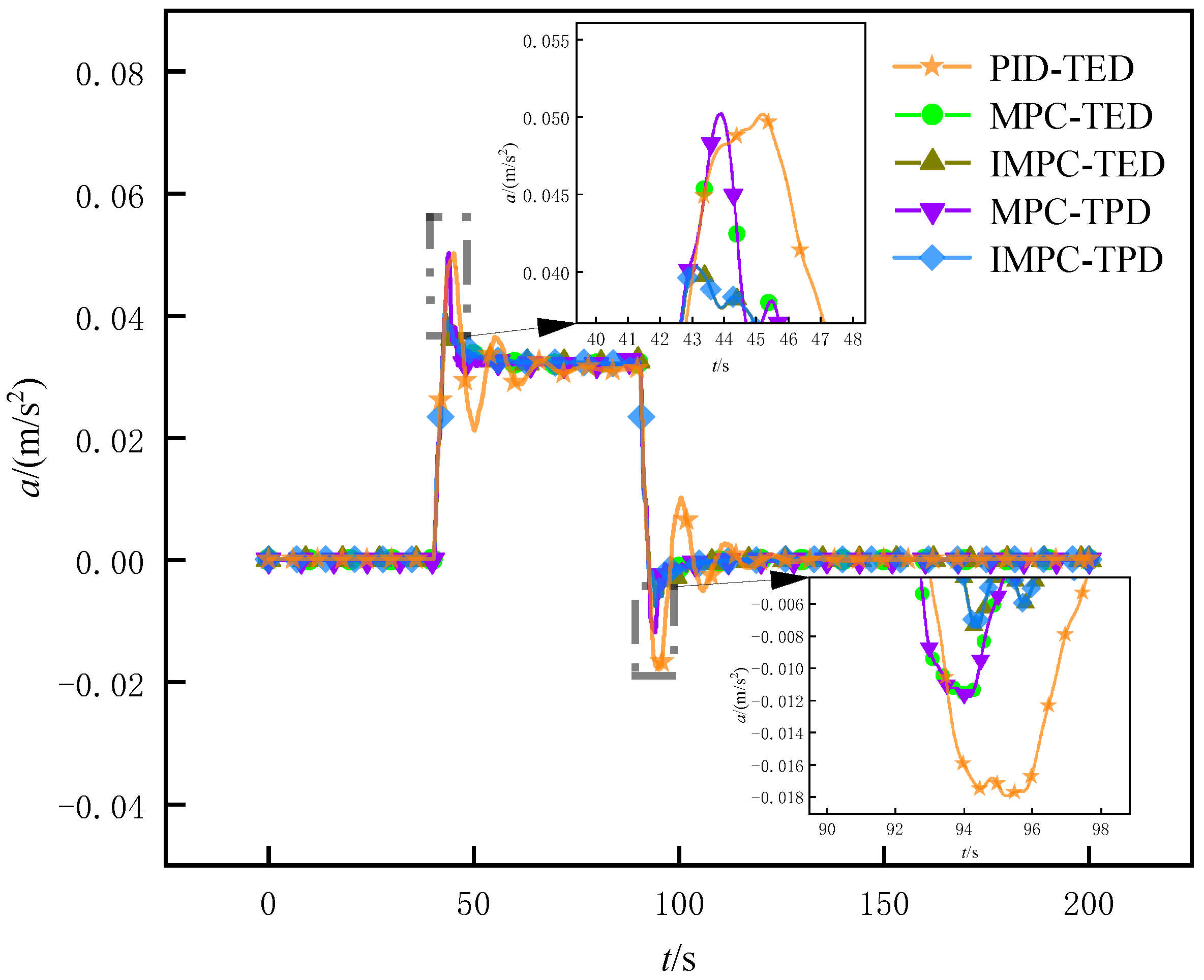
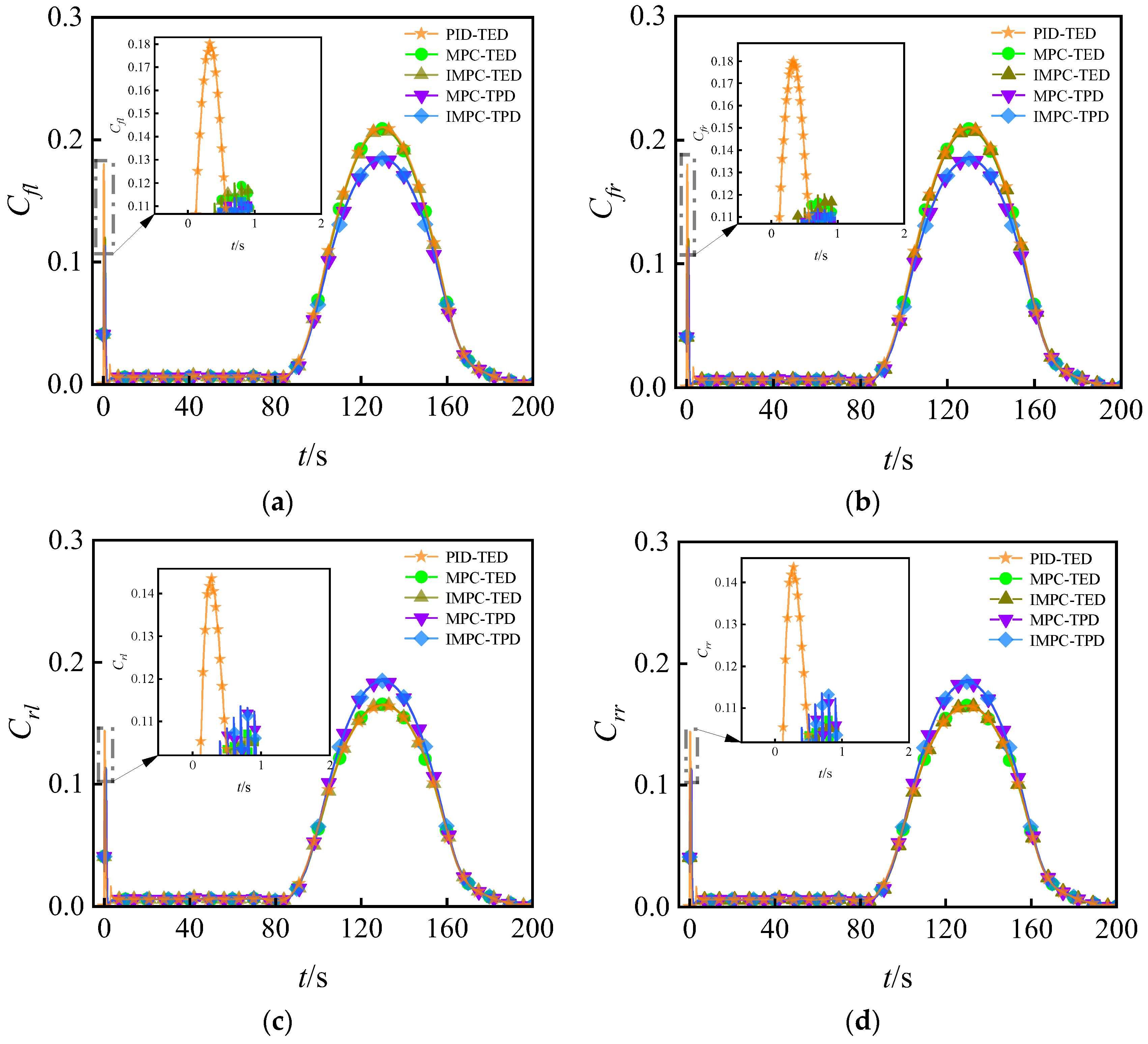
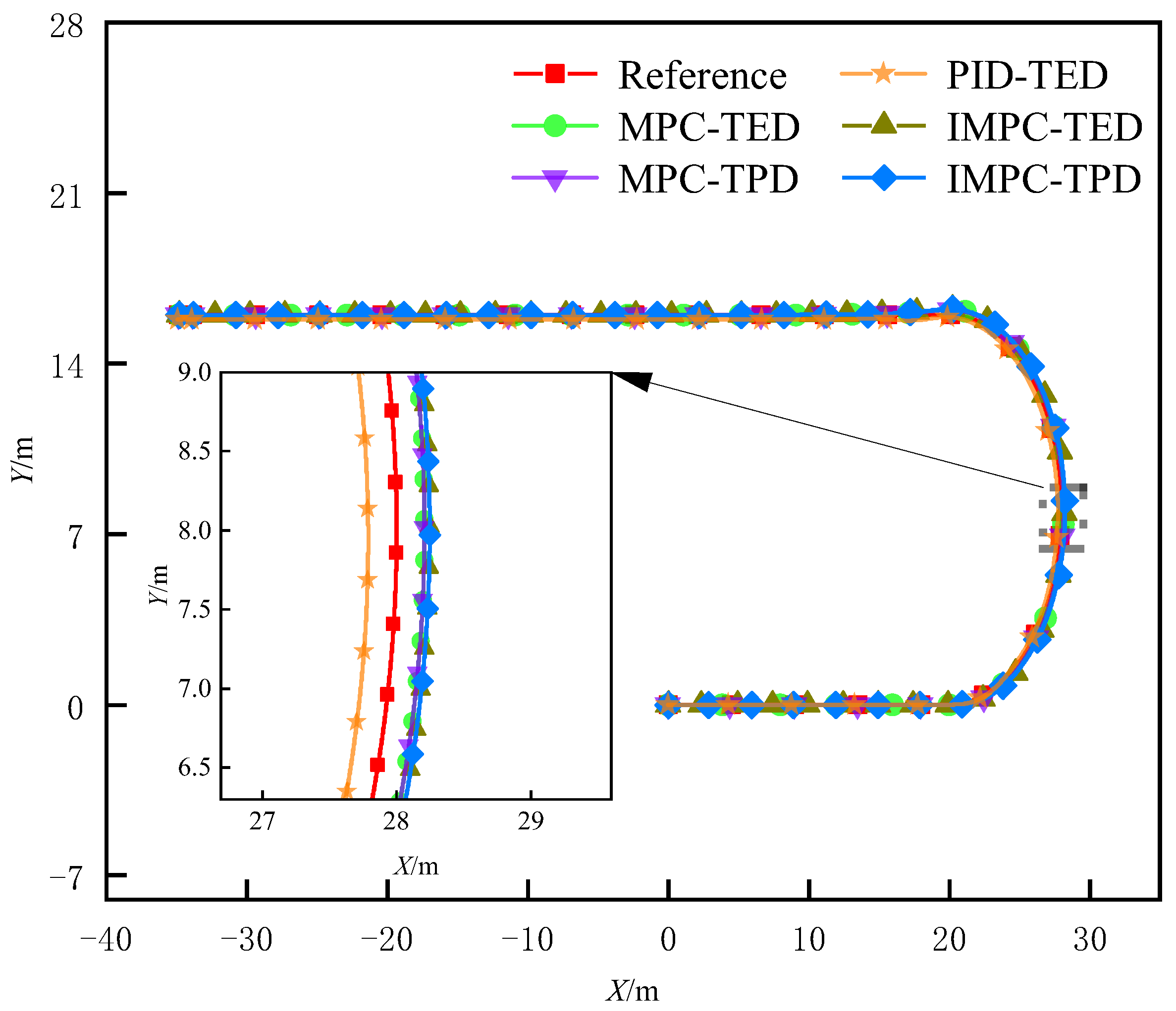
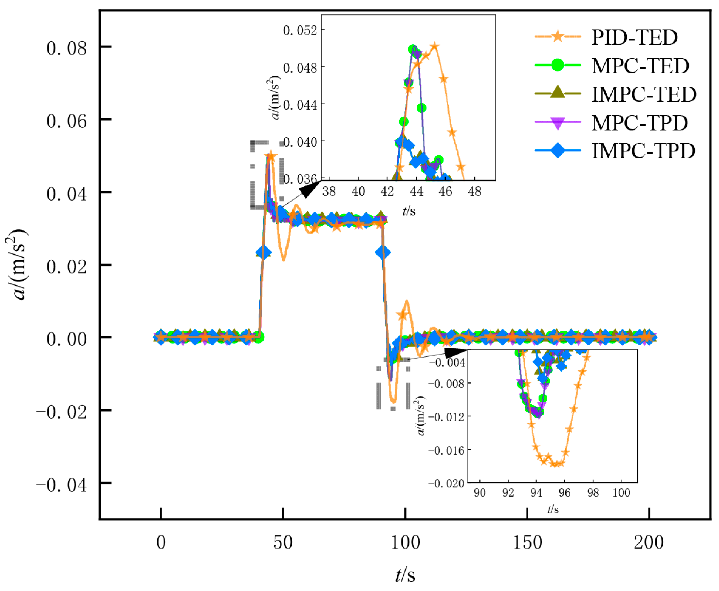
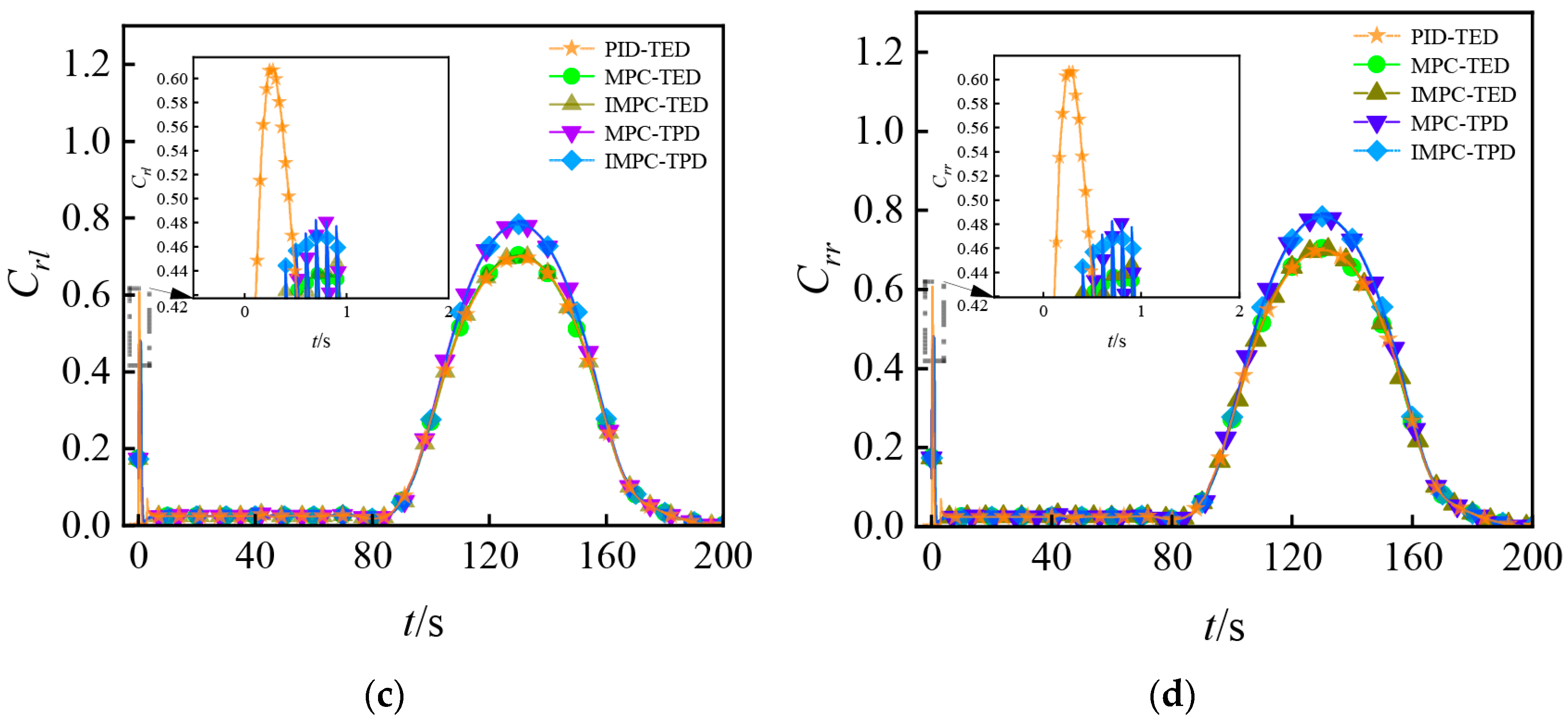
5.2. Simulation Results Extraction and Analysis

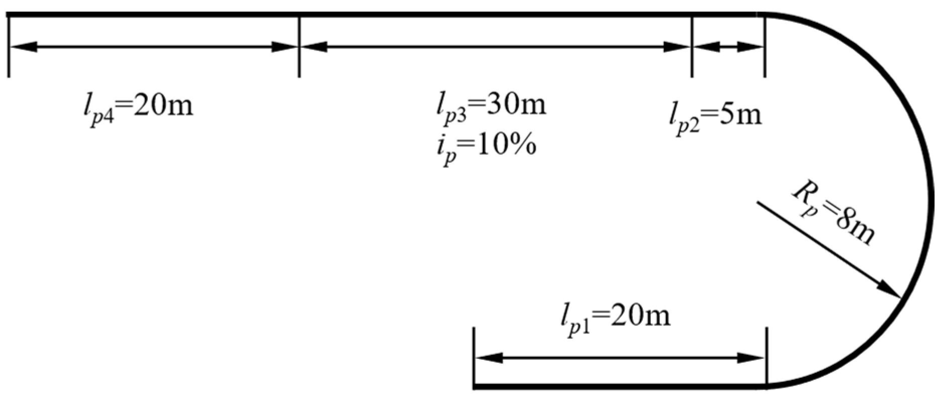
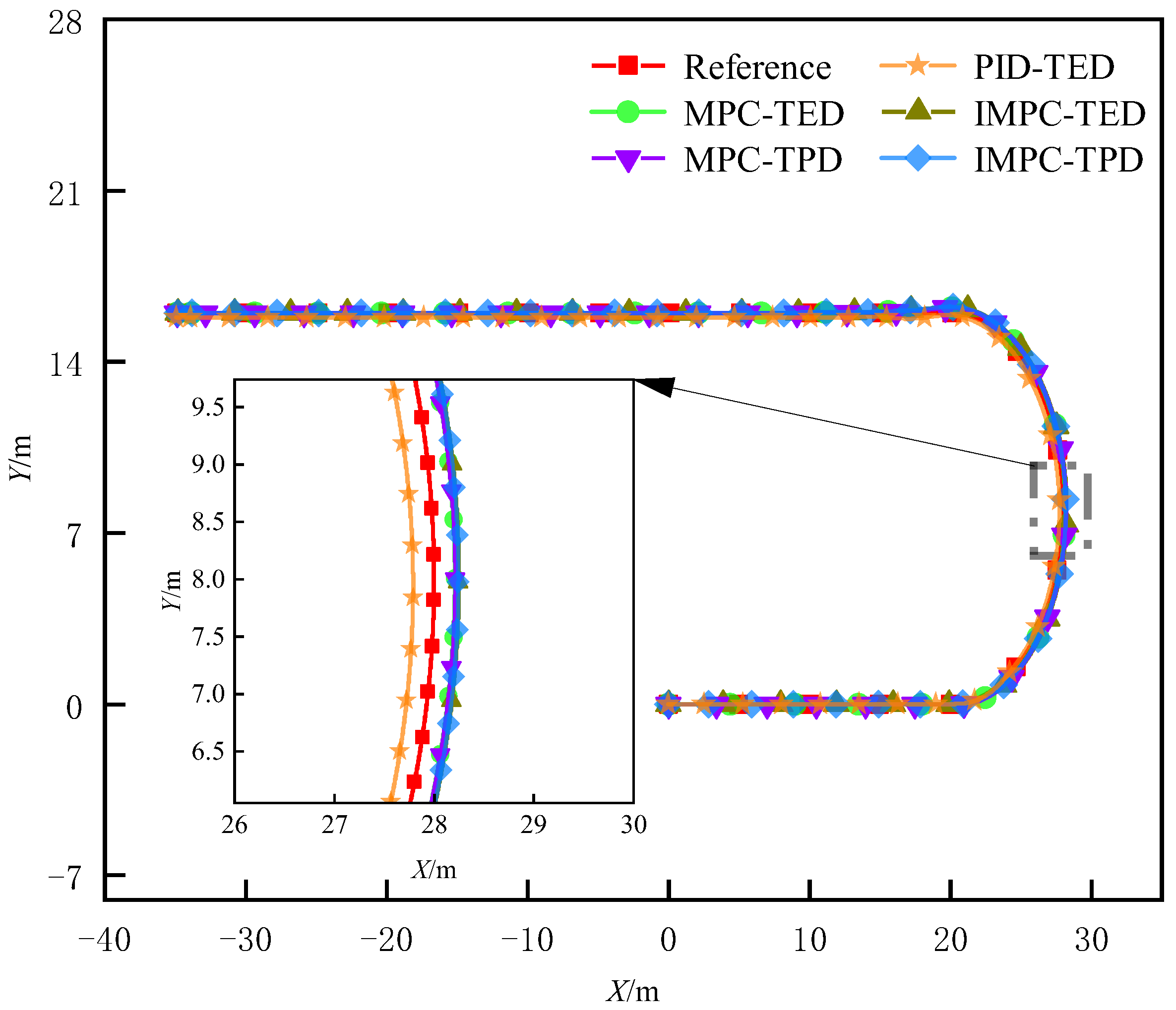
5.2.1. Trajectory Tracking Simulation Under High Pavement Adhesion Coefficient

High adhesion coefficient pavement is used to simulate the trajectory tracking performance of the AGV under dry outdoor factory pavement conditions. For dry asphalt or concrete pavements, the adhesion coefficient ranges from 0.8~0.9 [38]. With the mid-value selected, the pavement adhesion coefficient is set to 0.85. The prediction horizon and control horizon are set to 18 and 15, respectively. The evaluation parameters are extracted, including the maximum pose error |e_X|_max in the X-axis direction, the maximum pose error |e_Y|_max in the Y-axis direction, the maximum yaw angle error |e_Yaw|_max, the maximum lateral acceleration |a_y|_max and the maximum wheel adhesion rate C_max, as shown in

Table 3. Simulation results under high pavement adhesion coefficient.

Control Strategy		|eX|max/m	|eY|max/m	|eYaw|max/m	|ay|max/(m/s2)	Cmax
PID	PID-TED	0.2272	0.2419	0.0816	0.0502	0.2102
MPC	MPC-TED	0.2947	0.2132	0.0808	0.0502	0.2087
	MPC-TPD					0.1846
IMPC	IMPC-TED	0.2947	0.2492	0.0823	0.0403	0.2087
	IMPC-TPD					0.1846
comparison	IMPC and PID	29.7%	3.0%	0.9%	−19.7%	-
	IMPC and MPC	0	16.9%	1.9%	−19.7%	-
	TPD and TED	-	-	-	-	−11.5%

. The simulation results of the trajectory tracking curve, tracking error, lateral acceleration, wheel adhesion rate, and total driving torque of the front and rear wheels are shown in Figure 11, Figure 12, Figure 13 and Figure 14.

As can be seen from Figure 11 and Figure 12, since the reference vehicle speed remains constant while the actual vehicle speed starts from zero, a relatively large position tracking error occurs in the initial tracking stage. However, the control strategies using the MPC and IMPC controllers can quickly reduce the error. When the vehicle reaches the circular arc section, the reference wheel angle changes suddenly. To ensure the smooth change in the system control variables, the actual wheel angle increases gradually rather than suddenly, which leads to a certain pose tracking error during cornering. Nevertheless, the MPC and IMPC controllers can also quickly reduce the error. In contrast, the PID controller has a poorer performance. It can be seen from Table 3 that the control strategy using the IMPC controller has a slightly larger maximum tracking error compared with that using the MPC controller. This is because the IMPC controller considers the limitation of load transfer in the objective function, sacrificing a certain tracking accuracy. However, the control accuracy still meets the usage requirements.

As can be seen from Figure 13, a certain lateral acceleration is generated when the AGV is cornering. Since the steering angle of the AGV changes rapidly when entering and exiting the curve, there are certain extreme values of acceleration during these periods. As shown in Table 3, compared with the control strategy using the MPC controller, the maximum lateral acceleration of the control strategy using the IMPC controller is reduced by 22.40%. Compared with the control strategy using the PID controller, the maximum lateral acceleration is reduced by 19.7%. Therefore, on the pavement with a high adhesion coefficient, the improved MPC, namely the IMPC controller, achieves the goal of reducing the lateral load transfer.

As can be seen from Figure 14, during AGV startup and hill climbing, compared with the TED controller, the TPD controller reduces the front wheel adhesion rate while increasing the rear wheel adhesion rate. At the same time, the left-front and right-front wheels exhibit identical adhesion rates, as do the left-rear and right-rear wheels. This phenomenon arises because acceleration and slope during startup and climbing induce a rearward load transfer. The TPD controller automatically adjusts driving torque based on wheel-borne loads, resulting in smaller front-wheel torque and larger rear-wheel torque. Consequently, front-wheel adhesion decreases, rear-wheel adhesion increases, and maximum tire adhesion is reduced. As shown in Table 3, the maximum wheel adhesion rate decreases by 11.5%, demonstrating effective torque distribution.

5.2.2. Trajectory Tracking Simulation Under Low Pavement Adhesion Coefficient

The low-adhesion-coefficient pavement is used to simulate the trajectory tracking performance under the conditions of snowy, rainy, and slippery outdoor factory pavements. Since the adhesion coefficient of snow-covered pavements is 0.2, the pavement adhesion coefficient is set to 0.2. The prediction horizon and control horizon are set to 18 and 15, respectively. All the evaluation parameters and control strategy schemes are the same as those for the high-adhesion-coefficient pavement. The simulation results are shown in

Table 4. Simulation results under low pavement adhesion coefficient.

Control Strategy		|eX|max/m	|eY|max/m	|eYaw|max/m	|ay|max/(m/s2)	Cmax
PID	PID-TED	0.2273	0.2419	0.0816	0.0502	0.8934
MPC	MPC-TED	0.2947	0.2132	0.0808	0.0502	0.8871
	MPC-TPD					0.7847
IMPC	IMPC-TED	0.2947	0.2492	0.0823	0.0403	0.8871
	IMPC-TPD					0.7847
comparison	IMPC and PID	29.7%	3.0%	0.9%	−19.7%	-
	IMPC and MPC	0	16.9%	1.9%	−19.7%	-
	TPD and TED	-	-	-	-	−11.5%

and Figure 15, Figure 16, Figure 17 and Figure 18.

As can be seen from Figure 15, Figure 16 and Figure 17, the vehicle’s tracking performance, pose error, and maximum lateral acceleration during corner entry/exit on the low-adhesion coefficient pavement are nearly identical to those on the high-adhesion coefficient pavement. According to Table 4, the maximum lateral acceleration of the IMPC controller is reduced by 19.7% compared with both the MPC and PID controllers. Therefore, the IMPC controller also achieves the goal of reducing lateral load transfer on low-adhesion coefficient pavements.

As can be seen from Figure 18, on the low-adhesion coefficient pavement, during AGV startup and hill climbing, the TPD controller reduces the front wheel adhesion rate while increasing the rear wheel adhesion rate, and the maximum wheel adhesion rate is reduced, consistent with the high-adhesion coefficient pavement scenario. As shown in Table 4, the maximum wheel adhesion rate decreases by 11.6%, demonstrating effective torque distribution.

In summary, the control strategy proposed in this paper effectively reduces load transfer while ensuring tracking accuracy on both high- and low-adhesion coefficient pavements, achieves optimal torque distribution, and improves AGV driving stability, demonstrating ideal control performance.

6. Conclusions

To balance the trajectory tracking accuracy and stability of heavy-duty AGVs during operation, this paper takes outdoor heavy-duty AGVs transporting liquid-filled tonne and small drums as the research object. A trajectory tracking control strategy with load transfer control is proposed to reduce load transfer effects and improve driving stability and tracking accuracy. The main contributions are as follows:

• A 3-DOF kinematic model of the heavy-duty AGV is established. Through analysis of lateral and longitudinal load transfer under complex pavement conditions, the laws governing load transfer are derived;
• A control strategy considering both lateral and longitudinal load transfer is proposed. A lateral load-improved MPC controller based on lateral acceleration is designed alongside an adaptive torque distribution strategy according to longitudinal load transfer;
• Finally, a MATLAB/Simulink and CarSim co-simulation platform is built to conduct simulations on pavements with high and low adhesion coefficients. The results show that on both pavement types, the proposed control strategy effectively reduces vehicle lateral acceleration and lateral load transfer while maintaining tracking accuracy, decreases maximum tire adhesion rate, and improves driving stability, achieving ideal control performance for heavy-duty AGV.

References

1. Cheng, W.; Meng, W. An Efficient Genetic Algorithm for Multi AGV Scheduling Problem about Intelligent Warehouse. Robot. Intell. Automat. 2023, 43, 382–393. [Google Scholar] [CrossRef]
2. Li, K.; Liu, T.; Kumar, P.N.R.; Han, X. A Reinforcement Learning-Based Hyper-Heuristic for AGV Task Assignment and Route Planning in Parts-to-Picker Warehouses. Transp. Res. Part E Logist. Transp. Rev. 2024, 185, 103518. [Google Scholar] [CrossRef]
3. Liu, W.; Wan, Y.; Zhang, Q.; Yu, Y.; Liu, P.; Shi, Z. Trajectory Tracking Control of Four-Wheel Steering Automatic Guided Vehicle under the Working Condition of Moving Centroid. Proc. Inst. Mech. Eng. Part D J. Automob. Eng. 2023, 237, 691–705. [Google Scholar] [CrossRef]
4. Wang, Z.; Zeng, Q. A Branch-and-Bound Approach for AGV Dispatching and Routing Problems in Automated Container Terminals. Comput. Ind. Eng. 2022, 166, 107968. [Google Scholar] [CrossRef]
5. Jiang, J.; Zhang, S.; He, Y. Wheel Design and Motion Analysis of a New Heavy-Duty AGV in Aircraft Assembly Lines. Assem. Autom. 2020, 40, 387–397. [Google Scholar] [CrossRef]
6. Udengaard, M.; Iagnemma, K. Analysis, Design, and Control of an Omnidirectional Mobile Robot in Rough Terrain. J. Mech. Des. 2009, 131, 121002. [Google Scholar] [CrossRef]
7. Wang, K.; Liang, W.; Shi, H.; Zhang, J.; Wang, Q. Driving Line-Based Two-Stage Path Planning in the AGV Sorting System. Robot. Auton. Syst. 2023, 169, 104505. [Google Scholar] [CrossRef]
8. Yu, R.; Zhao, H.; Zhen, S.; Huang, K.; Chen, X.; Sun, H.; Shao, K. A Novel Trajectory Tracking Control of AGV Based on Udwadia-Kalaba Approach. IEEE/CAA J. Autom. Sin. 2024, 11, 1069–1071. [Google Scholar] [CrossRef]
9. Li, S.; Fan, L.; Jia, S. A Hierarchical Solution Framework for Dynamic and Conflict-Free AGV Scheduling in an Automated Container Terminal. Transp. Res. Part C Emerg. Technol. 2024, 165, 104724. [Google Scholar] [CrossRef]
10. Fu, W.J.; Liu, Y.; Zhang, X.M. Research on Accurate Motion Trajectory Control Method of Four-Wheel Steering AGV Based on Stanley-PID Control. Sensors 2023, 23, 7219. [Google Scholar] [CrossRef]
11. Li, S.; Zhou, Q.; Jiang, J.; Lu, X.; Yu, Z. MPC-Based Motion Control of AGV with Improved A* and Artificial Potential Field. Proc. Inst. Mech. Eng. Part D J. Automob. Eng. 2024, 239, 1035–1044. [Google Scholar] [CrossRef]
12. Chen, Z.; Fu, J.; Tu, X.-W.; Yang, A.-L.; Fei, M.-R. Real-Time Predictive Sliding Mode Control Method for AGV with Actuator Delay. Adv. Manuf. 2019, 7, 448–459. [Google Scholar] [CrossRef]
13. Lee, M.-Y.; Chen, B.-S. Robust H∞ Network Observer-Based Attack-Tolerant Path Tracking Control of Autonomous Ground Vehicle. IEEE Access 2022, 10, 58332–58353. [Google Scholar] [CrossRef]
14. Li, W.; Yu, S.; Tan, L.; Li, Y.; Chen, H.; Yu, J. Integrated Control of Path Tracking and Handling Stability for Autonomous Ground Vehicles with Four-Wheel Steering. Proc. Inst. Mech. Eng. Part D J. Automob. Eng. 2023, 239, 315–326. [Google Scholar] [CrossRef]
15. Wang, T.T.; Dong, R.Y.; Zhang, R.; Qin, D.C. Research on Stability Design of Differential Drive Fork-Type AGV Based on PID Control. Electronics 2020, 9, 1072. [Google Scholar] [CrossRef]
16. Zhai, J.Y.; Song, Z.B. Adaptive Sliding Mode Trajectory Tracking Control for Wheeled Mobile Robots. Int. J. Control 2019, 92, 2255–2262. [Google Scholar] [CrossRef]
17. Wu, X.; Jin, P.; Zou, T.; Qi, Z.Y.; Xiao, H.N.; Lou, P.H. Backstepping Trajectory Tracking Based on Fuzzy Sliding Mode Control for Differential Mobile Robots. J. Intell. Robot. Syst. 2019, 96, 109–121. [Google Scholar] [CrossRef]
18. Zhang, K.W.; Sun, Q.; Shi, Y. Trajectory Tracking Control of Autonomous Ground Vehicles Using Adaptive Learning MPC. IEEE Trans. Neural Netw. Learn. Syst. 2021, 32, 5554–5564. [Google Scholar] [CrossRef] [PubMed]
19. Yildiz, H.; Can, N.K.; Ozguney, O.C.; Yagiz, N. Sliding Mode Control of a Line Following Robot. J. Braz. Soc. Mech. Sci. Eng. 2020, 42, 561. [Google Scholar] [CrossRef]
20. Han, Y.X.; Cheng, Y.; Xu, G.W. Trajectory Tracking Control of AGV Based on Sliding Mode Control With the Improved Reaching Law. IEEE Access 2019, 7, 20748–20755. [Google Scholar] [CrossRef]
21. Wang, D.; Wei, W.; Yeboah, Y.; Li, Y.; Gao, Y. A Robust Model Predictive Control Strategy for Trajectory Tracking of Omni-directional Mobile Robots. J. Intell. Robot. Syst. 2020, 98, 439–453. [Google Scholar] [CrossRef]
22. Xing, B.; Xu, E.; Wei, J.; Meng, Y. Recurrent Neural Network Non-Singular Terminal Sliding Mode Control for Path Following of Autonomous Ground Vehicles with Parametric Uncertainties. IET Intell. Transp. Syst. 2022, 16, 616–629. [Google Scholar] [CrossRef]
23. Liu, K.; Gao, H.; Ji, H.; Hao, Z. Adaptive Sliding Mode Based Disturbance Attenuation Tracking Control for Wheeled Mobile Robots. Int. J. Control Autom. Syst. 2020, 18, 1288–1298. [Google Scholar] [CrossRef]
24. Chen, Z.; Liu, Y.; He, W.; Qiao, H.; Ji, H. Adaptive-Neural-Network-Based Trajectory Tracking Control for a Nonholonomic Wheeled Mobile Robot With Velocity Constraints. IEEE Trans. Ind. Electron. 2021, 68, 5057–5067. [Google Scholar] [CrossRef]
25. Wang, Y.; Sun, K.; Zhang, W.; Jin, X. A Velocity-Adaptive MPC-Based Path Tracking Method for Heavy-Duty Forklift AGVs. Machines 2024, 12, 558. [Google Scholar] [CrossRef]
26. Liu, Z.; Liu, G. Simulation and Test of Stability Control for Distributed Drive Electric Vehicles. Automot. Eng. 2019, 41, 792–799. [Google Scholar]
27. Fu, W.; Wang, X.; Zhang, X. Rollover Stability of Heavy-Duty AGVs in Turns Considering Variation in Friction Coefficient. Lubricants 2023, 11, 119. [Google Scholar] [CrossRef]
28. Zhang, Q.; Liu, W.; Liu, P. Fault-Tolerant Control of Automated Guided Vehicle Under Centroid Variation. IEEE Access 2022, 10, 68995–69009. [Google Scholar] [CrossRef]
29. Liu, W.; Zhang, Q.; Wan, Y.; Liu, P.; Yu, Y.; Guo, J. Yaw Stability Control of Automated Guided Vehicle under the Condition of Centroid Variation. J. Braz. Soc. Mech. Sci. Eng. 2022, 44, 18. [Google Scholar] [CrossRef]
30. Liu, X.; Wang, G.; Chen, K. Nonlinear Model Predictive Tracking Control With C/GMRES Method for Heavy-Duty AGVs. IEEE Trans. Veh. Technol. 2021, 70, 12567–12580. [Google Scholar] [CrossRef]
31. Hwang, C.-L.; Yang, C.-C.; Hung, J.Y. Path Tracking of an Autonomous Ground Vehicle With Different Payloads by Hierarchical Improved Fuzzy Dynamic Sliding-Mode Control. IEEE Trans. Fuzzy Syst. 2018, 26, 899–914. [Google Scholar] [CrossRef]
32. Sun, Z.; Xie, H.; Zheng, J.; Man, Z.; He, D. Path-Following Control of Mecanum-Wheels Omnidirectional Mobile Robots Using Nonsingular Terminal Sliding Mode. Mech. Syst. Signal Proc. 2021, 147, 107128. [Google Scholar] [CrossRef]
33. Liu, W.; Yu, Y.; Wan, Y. Rollover Control of AGV Combined with Differential Drive, Active Steering, and Centroid Adjustment under Slope Driving Condition. Math. Probl. Eng. 2022, 2022, 9331756. [Google Scholar] [CrossRef]
34. Nguyen, V.; Schultz, G.; Balachandran, B. Lateral Load Transfer Effects on Bifurcation Behavior of Four-Wheel Vehicle System. J. Comput. Nonlinear Dyn. 2009, 4, 041007. [Google Scholar] [CrossRef]
35. Yue, M.; Yang, L.; Sun, X.-M.; Xia, W. Stability Control for FWID-EVs With Supervision Mechanism in Critical Cornering Situations. IEEE Trans. Veh. Technol. 2018, 67, 10387–10397. [Google Scholar] [CrossRef]
36. Mutoh, N. Driving and Braking Torque Distribution Methods for Front- and Rear-Wheel-Independent Drive-Type Electric Vehicles on Roads With Low Friction Coefficient. IEEE Trans. Ind. Electron. 2012, 59, 3919–3933. [Google Scholar] [CrossRef]
37. De Novellis, L.; Sorniotti, A.; Gruber, P. Wheel Torque Distribution Criteria for Electric Vehicles With Torque-Vectoring Differentials. IEEE Trans. Veh. Technol. 2014, 63, 1593–1602. [Google Scholar] [CrossRef]
38. Yu, Z.; Xia, Q. Automobile Theory, 6th ed.; China Machine Press: Beijing, China, 2018; pp. 114–120. [Google Scholar]
Figure 1. Three-dimensional model of heavy-duty AGV: 1—Drive module; 2—Control module; 3—Power module; 4—Lift module; 5—Ladar.
Applsci 15 04512 g001
Figure 2. Double Ackerman steering model.
Applsci 15 04512 g002
Figure 3. Kinematics model of bicycle.
Applsci 15 04512 g003
Figure 4. Steering trapezoid diagram.
Applsci 15 04512 g004
Figure 5. The simplified model of AGV during lateral load transfer is analyzed: (a) I-shaped frame force diagram; (b) lateral force balance diagram; (c) front axle force diagram; (d) rear shaft force diagram.
Applsci 15 04512 g005
Figure 6. Simplified model of AGV during longitudinal load transfer.
Applsci 15 04512 g006
Figure 7. The structure diagram of the control system.
Applsci 15 04512 g007
Figure 8. Structure diagram of torque adaptive distribution control strategy.
Applsci 15 04512 g008
Figure 9. Simulink and CarSim co-simulation model.
Applsci 15 04512 g009
Figure 10. Reference trajectory.
Applsci 15 04512 g010
Figure 11. Trajectory tracking curve.
Applsci 15 04512 g011
Figure 12. Tracking error curve: (a) X-axis direction error; (b) Y-axis direction error; (c) maximum yaw angle error.
Applsci 15 04512 g012
Figure 13. Lateral acceleration curve.
Applsci 15 04512 g013
Figure 14. Adhesion rate curve of each wheel: (a) left front wheel; (b) right front wheel; (c) left rear wheel; (d) right rear wheel.
Applsci 15 04512 g014
Figure 15. Trajectory tracking curve.
Applsci 15 04512 g015
Figure 16. Tracking error curve: (a) X-axis direction error; (b) Y-axis direction error; (c) maximum yaw angle error.
Applsci 15 04512 g016
Figure 17. Lateral acceleration curve.
Applsci 15 04512 g017
Figure 18. Adhesion rate curve of each wheel: (a) left front wheel; (b) right front wheel; (c) left rear wheel; (d) right rear wheel.
Applsci 15 04512 g018aApplsci 15 04512 g018b