Increasing the Classification Achievement of Steel Surface Defects by Applying a Specific Deep Strategy and a New Image Processing Approach

Abstract

Defect detection is still challenging to apply in reality because the goal of the entire classification assignment is to identify the exact type and location of every problem in an image. Since defect detection is a task that includes location and categorization, it is difficult to take both accuracy factors into account when designing related solutions. Flaw detection deployment requires a unique detection dataset that is accurately annotated. Producing steel free of flaws is crucial, particularly in large production systems. Thus, in this study, we proposed a novel deep learning-based flaw detection system with an industrial focus on automated steel surface defect identification. To create processed images from raw steel surface images, a novel method was applied. A new deep learning model called the Parallel Attention–Residual CNN (PARC) model was constructed to extract deep features concurrently by training residual structures and attention. The Iterative Neighborhood Component Analysis (INCA) technique was chosen for distinguishing features to lower the computational cost. The classification assessed the SVM method using a convincing dataset (Severstal: Steel Defect Detection). The accuracy in both the binary and multi-class classification tests was above 90%. Moreover, using the same dataset, the suggested model was contrasted with pre-existing models.

1. Introduction

Improving productivity and preserving product quality are crucial in production systems [1]. One of the most crucial aspects of quality control is the detection of surface defects. Traditional detection techniques rely on expert inspection for control, which has disadvantages such as time wastage, poor productivity, and poor reliability [2]. Specifically, automatic surface defect detection is becoming increasingly important in steel industries having extensive production fields. Due to heat treatment, non-metallic inclusion, corrosion, and emulsification, flat-rolled steel can develop flaws such as cracks, pitted surfaces, scratches, and patches [3]. Evaluating defect geometry and generating a sizable sample of statistical data is crucial for improving the surface defect process. As a consequence, automated detection and classification systems can prevent unforeseen equipment failure.

Automatic surface defect detection has frequently been accomplished using traditional machine learning and deep learning-based techniques [4]. Conventional classification approaches including model-based, statistical-based, and spectral-based methods typically rely on statistical data and visual features. These techniques, such as thresholding, Sobel, Local Binary Patterns (LBPs), Fourier transform, and Canny’s algorithm, are used to convert features obtained manually, but factors including the background, lighting, and camera angle directly impact the effectiveness of defect identification [5]. Additionally, these techniques have limitations when used on various surfaces, making them unsuitable for use in practical situations [6]. Deep learning-based methods are now used to improve defect-detection capabilities in computer vision [7]. When using deep learning techniques, the algorithm can function by producing prompt and precise predictions even in the absence of supervision. Thus, labor and time saving by detecting automatically in the steel factories have made important advantages in comparison with manual control by technicians and engineers [8].

2. Related Studies

The number of studies using machine learning to identify surface defects of steel has increased during the past few years. Martins et al. [9] performed automatic surface fault detection of rolled steel using artificial neural networks with image processing. The classification of certain defects, including clamps, holes, and welding, was detected by the image analysis Hough Transform method, while other complicated defects, such as exfoliation, oxidation, and waveform, were detected by applying Self-Organizing Maps and Principal Component Analysis to extract features. The system achieved an overall accuracy of 87% after managing real-world datasets. Li et al. [10] designed a feature fusion-based method to improve steel surface defect detection in their proposed model. In this method, a multiscale feature extraction (MSFE) strategy is adopted from a YOLO-based model. With the MSFE algorithm, features with different scales are extracted from multidimensional kernels of different convolution layers. An efficient feature fusion technique is then used to maximize feature discriminability. This model, developed on the publicly available NEU-DET dataset, achieved an optimum accuracy of 73.08%. Pang and Tan [11] developed a graph neural network-based method for detecting steel surface defects. They also used a novel attention mechanism called HDmA in this approach. This strategy was also successful in detecting defects in different fields of view. This method was tested on NEU-DET and GC-10 datasets and achieved 79.04% and 66.93% accuracy, respectively. Zhang et al. [12] presented a model based on YOLO v5 for detecting defects on steel surfaces. A multi-feature fusion technique, Res2Attention blocks, was used to improve the performance of the model. Model performance was tested on the NEU-DET and GC10-DET datasets. The classification accuracies were 78.5% and 67.3%, respectively. A vision-based automatic detection method with three-section defect detection, region extraction, and industrial liquid quantification was proposed by Zhao et al. [13]. They discovered that industrial liquids were measured with an accuracy rate of 90%. The accuracy rate of the recognition of cracks and scratches was obtained as 91% or more. By creating a dataset with six defects: scars, scratches, inclusions, burrs, seams, and iron scales. Li et al. [14] explored the surface defect recognition of steel strips by converting You Only Look Once (YOLO) completely into convolutional layers. The rates of detection, recall, and mAP were 99%, 95.86%, and 97.55%, respectively. Fu et al. [15] applied the SqueezeNet model by pre-training on the dataset of ImageNet for the classification of six different defects, which are rolled-in scales, inclusions, patches, scratches, crazing, and pitted surfaces. They came to the conclusion that the learned features significantly outperformed the hand-crafted ones for datasets that were heterogeneous and unseen. By using the strong time-sequenced properties of defects, Liu et al. [16] studied steel defect detection periodically by using a convolutional neural network (CNN) and a long short-term memory (LSTM) to detect roll mark defects. After extracting the defect features of samples with CNN, vectors were added to the long- and short-term memory to detect defects. As a result, the proposed method reached 81.9% of the performance of defect detection and outperformed the CNN approach. The performance of the system was raised to a rate of 6.2% by enhancing the attention mechanism. Liu et al. [17] utilized the dataset of NEU-CLS to improve the concurrent convolutional neural network (ConCNN) with light weight by using different scales of samples. The method’s accuracy performance was found to be 98.89% with a duration of 5.58 ms. The classification pre-training of surface defects was conducted using VGG19 by Guan et al. [18]. Feature extraction from the various levels of the defect weight model was performed using VGG19. Following that, SSIM and a Decision Tree were used to estimate the structure of VGG19 and the quality of the feature picture. The experiment used a dataset from Northeast University with six different types of steel surface defects, crazing, inclusions, patches, pitted surfaces, rolled-in scales, and scratches, each with 300 samples and a total of 1800 grayscale images. Following 23,000 steps, it was discovered that the VSD model’s validation rate was 89.86% higher than that of ResNet and VGG19. By using U-net and Deep Residual techniques for the classification of four different defects, Amin and Akhter [19] concluded that their system performances were 0.731 and 0.543 in terms of the Dice coefficient accuracy, respectively. In total, 12,568 training images and 1801 test images were created with a 1600 × 256 × 1 image size. A privacy dataset was explored by Zhao et al. [3] utilizing enhanced Faster R-CNN. By enhancing the conventional Faster R-CNN algorithm, the network structure of the Faster R-CNN was rebuilt. Following the testing, upgraded Faster R-CNN was proven to have a greater mean average accuracy performance for crazing, inclusions, patches, rolled-in scales, and pitted surface defect types with the following values of 0.501, 0.791, 0.792, 0.905, and 0.649, respectively.

After a detailed search of datasets studied at the academic level, it was understood that studies of classification are limited to surface defect detection and classification. However, surface flaws in real-world practices often affect only a small portion of the overall steel surface. As a result, using such data makes success more challenging. Because the Steel Surface Defect Database is a difficult dataset, a deep learning-based strategy that will perform well with it is used in this work.

3. Literature Gap, Motivation, and Contributions

To summarize the literature in general, in terms of deep learning, pre-trained models or lightweight CNN models have been used to classify defects on steel surfaces. Additionally, no frequency–time conversion algorithm has been used to increase the discrimination in the images. Looking at the literature, it is evident that many deep learning-based studies have been conducted to minimize defects in steel production. In studies focusing on the classification problem, the classification accuracy ranged between 80% and 90%. Especially in YOLO-based fault detection studies, the classification accuracy performance was between 65% and 75%. When these accuracy values are considered, it is obvious that the error performance of steel surfaces is still open to improvement. In a steel mill with a high production capacity, even a 2–3% increase in the defect detection performance will significantly improve the production quality. Therefore, there is a serious need for a deep learning-based application that detects steel surface defects with high performance.

This study was carried out to distinguish and classify defects on steel surfaces, as a small improvement in defect detection in high-capacity steel production will provide a large number of defect-free steel products. The proposed approach is designed in four main stages. The first stage is the processing of raw images. The second stage is responsible for extracting features from the Parallel Attention–Residual CNN (PARC) model. The third stage involves feature selection with the Iterative Neighborhood Component Analysis (INCA) algorithm. The final stage includes classification with a powerful algorithm. The proposed approach has three important contributions, as outlined below.

• Attention and residual structures in the CNN model were added to the PARC model and trained in parallel. This increased the representation power of the features extracted from the PARC model. Therefore, the classification performance was improved. Although the parallel integration of attention and residual blocks has been studied in previous works, our proposed PARC architecture introduces a distinct combination specifically tailored for defect recognition in steel surface images. To validate its superiority, we conducted comparative experiments against baseline CNNs with only residual blocks, only attention modules, and sequential Attention–Residual designs. The results demonstrate that PARC achieves a consistently higher accuracy and robustness across both multi-class and binary classification tasks.
• Raw images were processed with a new approach. In this approach, 1D stack data are used instead of a signal to obtain spectrogram images. For 1D stack data, the gradient of the raw images was taken and then converted into sequential 1D stack data. The gradient operation highlighted the differences in pixel values in the image. As a result, the classification performance is improved with this pre-processing procedure. Existing methods all use pixel data. In this study, thanks to the transformation of the image into 1D stack data, it was possible to access the frequency information of images that form a pattern with each other, such as scratches and cracks. In this case, it increased the classification performance compared to raw images.

4. Dataset

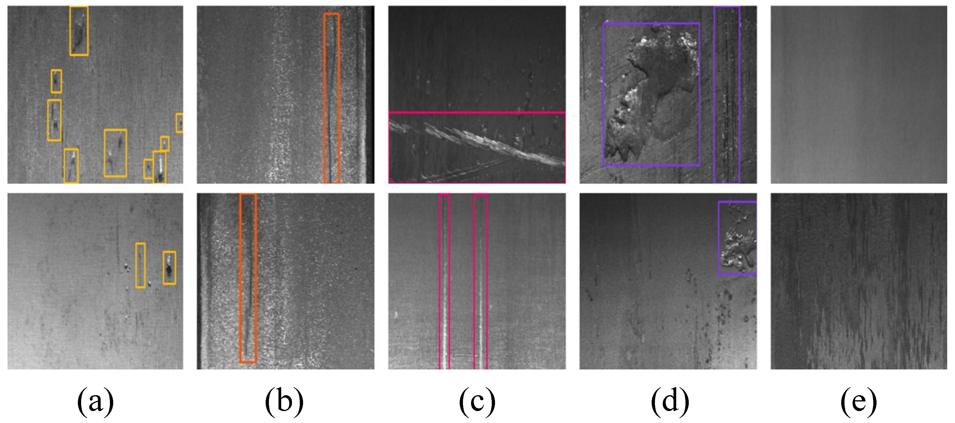
The suggested methodology was tested using a challenging dataset from the Kaggle database called Severstal: Steel Defect Detection (2019) [20]. Two tasks involving binary and multi-class classification used the dataset. Images of steel faults (6666 images) and images of no defects (5902 images), obtained using specialized imaging equipment to identify defects, were employed in the binary classification. The multi-class classification work used 6668 steel defect images with pitted surfaces, crazing, scratches, patches, and multi-defect class labels. Each sample of the collection was saved as a 1600 × 256 JPG image. To lessen the hardware requirements for this study, each sample was re-saved in a size of 200 × 32. Figure 1 shows a few samples for each class.

5. Proposed Methodology

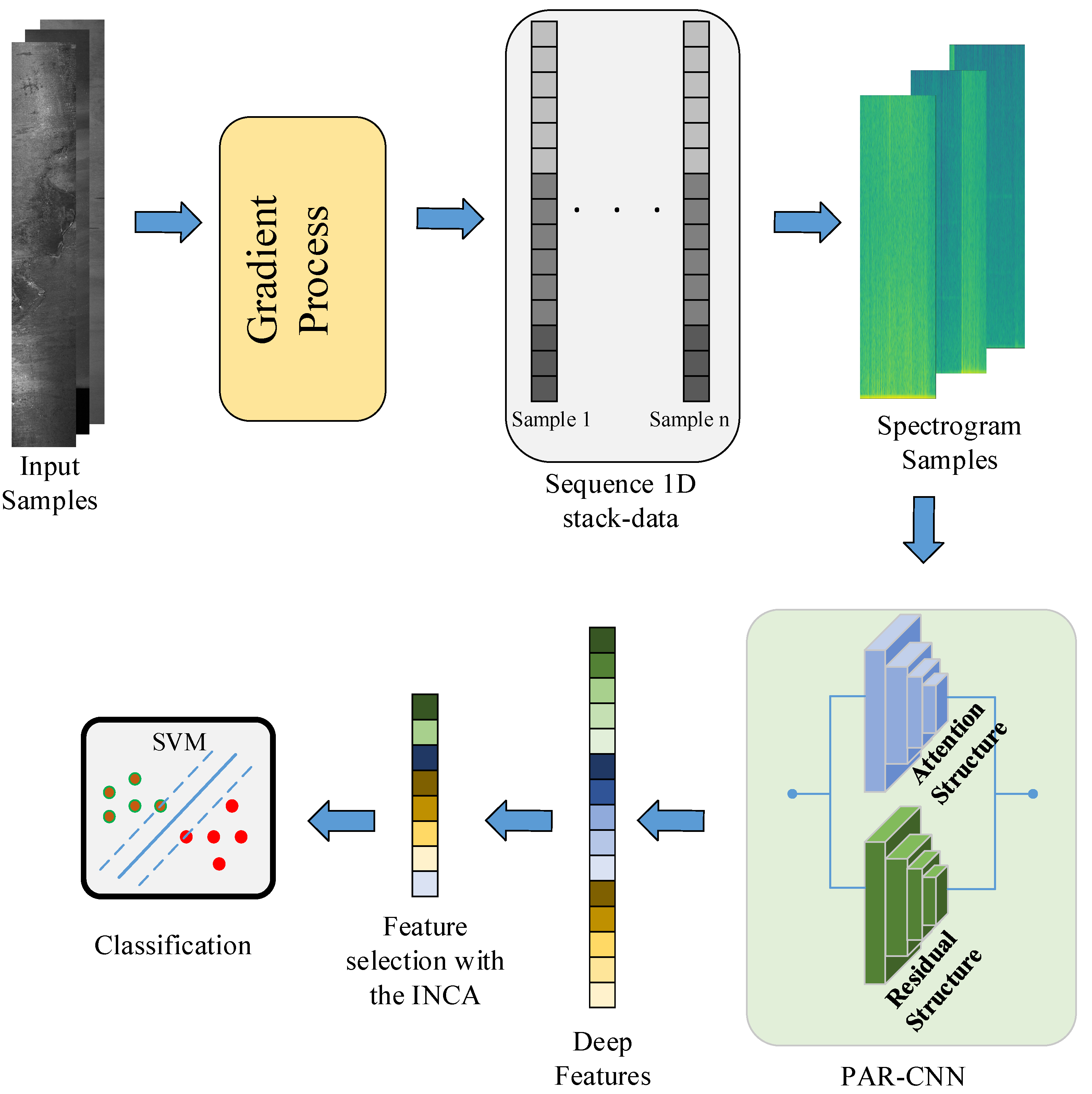
The methodology of this study introduces a novel and robust approach to enhance the classification performance for surface defect detection, consisting of five distinct yet interconnected stages. Figure 2 shows the representation of the proposed approach. The innovative aspect of the approach begins with the pre-processing of raw images, where a unique method is employed. Unlike traditional image pre-processing techniques, this study applies a spectrogram algorithm to time series signals derived from images that contain surface defects. This step transforms 2D image data into a 1D stack by utilizing pixel values, enabling the extraction of spectrogram images. This novel transformation provides a powerful representation of pixel variations in defect regions, enhancing the model’s ability to capture subtle details crucial for classification.

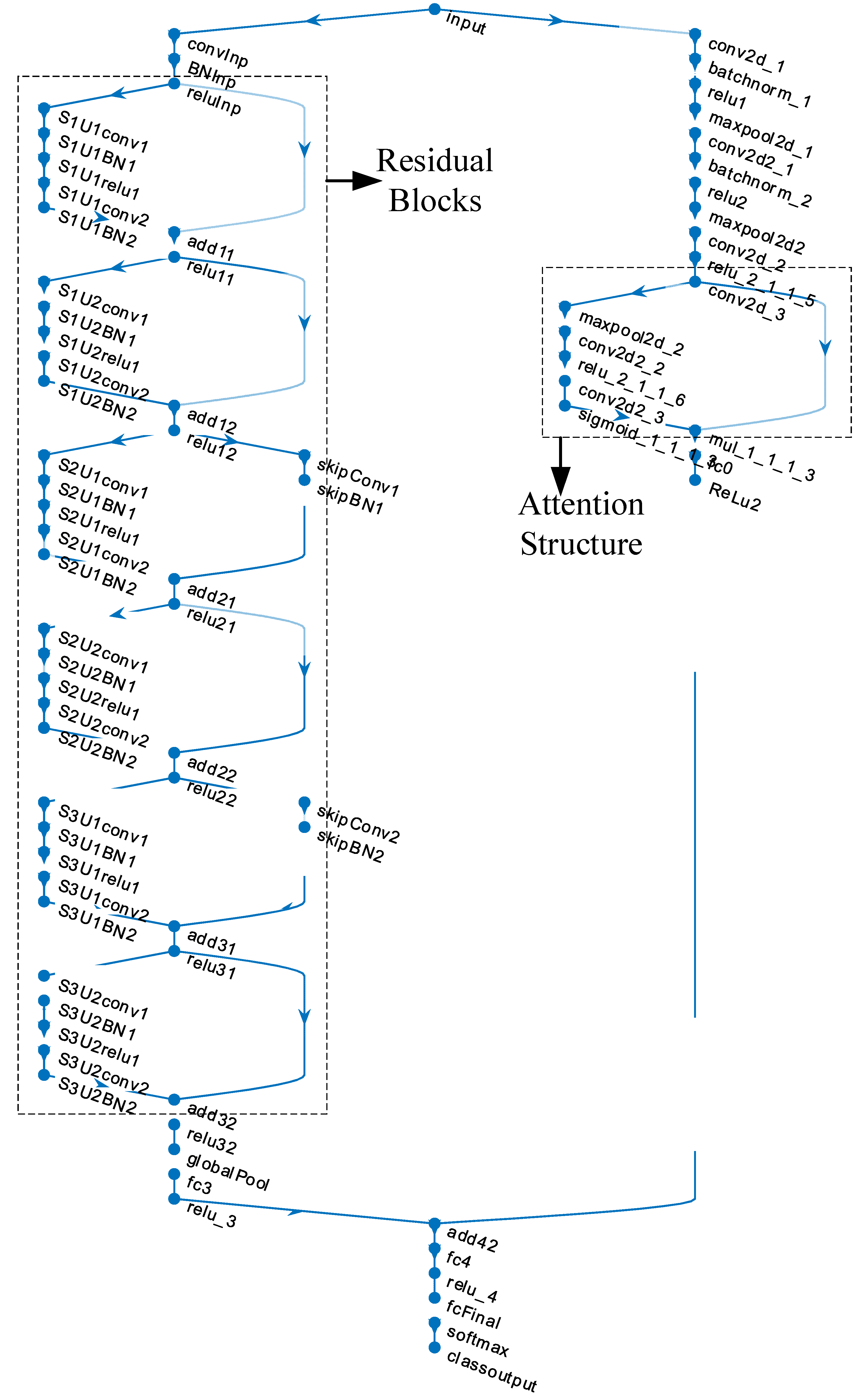
In the second stage, the processed spectrogram images are used to train a newly designed architecture known as the Parallel Attention–Residual CNN (PARC) model. Figure 3 shows the layer connections of the PARC model. The innovation in this model lies in its dual use of attention and residual mechanisms within a customized CNN framework, operating in parallel. Attention mechanisms focus on emphasizing critical areas within the image, while residual connections allow the preservation of feature information from earlier layers by passing it forward to subsequent layers. This synergy ensures that vital details, which may have otherwise been diminished or lost in deep layers, are retained and utilized, thus improving the learning capability of the network. While state-of-the-art architectures such as Swin Transformer, EfficientNetV2, and YOLOv7 have demonstrated remarkable performance across a variety of vision tasks, they are primarily designed as general-purpose models and often involve high computational costs and large parameter counts. In contrast, the proposed PARC (Parallel Attention and Residual Convolution) model is specifically tailored for steel surface defect recognition, focusing on enhancing subtle and fine-grained texture variations that are commonly present in such industrial inspection tasks. The parallel integration of attention and residual mechanisms in PARC enables it to capture both local defect features and global structural information more effectively, without significantly increasing the computational complexity. Compared to Transformer-based models like Swin Transformer, which require large datasets and extensive training resources to generalize well, PARC achieves a competitive or superior accuracy with a lightweight and task-optimized architecture. Furthermore, unlike YOLOv7, which is object-detection-focused and might exhibit overkill or be less efficient for fine-grained classification tasks, PARC offers a better balance between precision, speed, and model complexity. Its compact design makes it more suitable for real-time deployment in edge environments commonly found in industrial inspection systems. Detailed layer information of the PARC model is given in

Table A1. Layers of the PARC model.

Layer	Layer Order	Layer	Layer Info
1	‘conv2d_1’	2D Convolution	In total, 16 5 × 5 × 3 convolutions with stride [1 1] and padding ‘same’
2	‘batchnorm_1’	Batch Normalization	Batch normalization with 16 channels
3	‘relu1’	ReLU	ReLU
4	‘maxpool2d_1’	2D Max Pooling	In total, 2 × 2 max pooling with stride [1 1] and padding [0 0 0 0]
5	‘conv2d2_1’	2D Convolution	In total, 8 3 × 3 × 16 convolutions with stride [1 1] and padding ‘same’
6	‘batchnorm_2’	Batch Normalization	Batch normalization with 8 channels
7	‘relu2’	ReLU	ReLU
8	‘maxpool2d2’	2D Max Pooling	In total, 2 × 2 max pooling with stride [1 1] and padding [0 0 0 0]
9	‘conv2d_2’	2D Convolution	In total, 8 2 × 2 × 8 convolutions with stride [1 1] and padding ‘same’
10	‘relu_2_1_1_5’	ReLU	ReLU
11	‘conv2d_3’	2D Convolution	In total, 8 3 × 3 × 8 convolutions with stride [1 1] and padding ‘same’
12	‘maxpool2d_2’	2D Max Pooling	In total, 2 × 2 max pooling with stride [1 1] and padding ‘same’
13	‘conv2d2_2’	2D Convolution	In total, 8 5 × 5 × 8 convolutions with stride [1 1] and padding ‘same’
14	‘relu_2_1_1_6’	ReLU	ReLU
15	‘conv2d2_3’	2D Convolution	In total, 8 3 × 3 × 8 convolutions with stride [1 1] and padding ‘same’
16	‘sigmoid_1_1_1_3’	sigmoidLayer	sigmoidLayer
17	‘mul_1_1_1_3’	ElementWiseMultiplication	Element-Wise Multiplication of 2 inputs
18	‘fc0’	Fully Connected	In total, 350 fully connected layers
19	‘ReLu2’	ReLU	ReLU
20	‘input’	Image Input	In total, 32 × 200 × 3 images with ‘zero center’ normalization
21	‘convInp’	2D Convolution	In total, 16 3 × 3 × 3 convolutions with stride [1 1] and padding ‘same’
22	‘BNInp’	Batch Normalization	Batch normalization with 16 channels
23	‘reluInp’	ReLU	ReLU
24	‘S1U1conv1’	2D Convolution	In total, 16 3 × 3 × 16 convolutions with stride [1 1] and padding ‘same’
25	‘S1U1BN1’	Batch Normalization	Batch normalization with 16 channels
26	‘S1U1relu1’	ReLU	ReLU
27	‘S1U1conv2’	2D Convolution	In total, 16 3 × 3 × 16 convolutions with stride [1 1] and padding ‘same’
28	‘S1U1BN2’	Batch Normalization	Batch normalization with 16 channels
29	‘add11’	Addition	Element-wise addition of 2 inputs
30	‘relu11’	ReLU	ReLU
31	‘S1U2conv1’	2D Convolution	In total, 16 3 × 3 × 16 convolutions with stride [1 1] and padding ‘same’
32	‘S1U2BN1’	Batch Normalization	Batch normalization with 16 channels
33	‘S1U2relu1’	ReLU	ReLU
34	‘S1U2conv2’	2D Convolution	In total, 16 3 × 3 × 16 convolutions with stride [1 1] and padding ’same’
35	‘S1U2BN2’	Batch Normalization	Batch normalization with 16 channels
36	‘add12’	Addition	Element-wise addition of 2 inputs
37	‘relu12’	ReLU	ReLU
38	‘S2U1conv1’	2D Convolution	In total, 32 3 × 3 × 16 convolutions with stride [2 2] and padding ‘same’
39	‘S2U1BN1’	Batch Normalization	Batch normalization with 32 channels
40	‘S2U1relu1’	ReLU	ReLU
41	‘S2U1conv2’	2D Convolution	In total, 32 3 × 3 × 32 convolutions with stride [1 1] and padding ‘same’
42	‘S2U1BN2’	Batch Normalization	Batch normalization with 32 channels
43	‘add21’	Addition	Element-wise addition of 2 inputs
44	‘relu21’	ReLU	ReLU
45	‘S2U2conv1’	2D Convolution	In total, 32 3 × 3 × 32 convolutions with stride [1 1] and padding ‘same’
46	‘S2U2BN1’	Batch Normalization	Batch normalization with 32 channels
47	‘S2U2relu1’	ReLU	ReLU
48	‘S2U2conv2’	2D Convolution	In total, 32 3 × 3 × 32 convolutions with stride [1 1] and padding ‘same’
49	‘S2U2BN2’	Batch Normalization	Batch normalization with 32 channels
50	‘add22’	Addition	Element-wise addition of 2 inputs
51	‘relu22’	ReLU	ReLU
52	‘S3U1conv1’	2D Convolution	In total, 64 3 × 3 × 32 convolutions with stride [2 2] and padding ‘same’
53	‘S3U1BN1’	Batch Normalization	Batch normalization with 64 channels
54	‘S3U1relu1’	ReLU	ReLU
55	‘S3U1conv2’	2D Convolution	In total, 64 3 × 3 × 64 convolutions with stride [1 1] and padding ‘same’
56	‘S3U1BN2’	Batch Normalization	Batch normalization with 64 channels
57	‘add31’	Addition	Element-wise addition of 2 inputs
58	‘relu31’	ReLU	ReLU
59	‘S3U2conv1’	2D Convolution	In total, 64 3 × 3 × 64 convolutions with stride [1 1] and padding ‘same’
60	‘S3U2BN1’	Batch Normalization	Batch normalization with 64 channels
61	‘S3U2relu1’	ReLU	ReLU
62	‘S3U2conv2’	2D Convolution	In total, 64 3 × 3 × 64 convolutions with stride [1 1] and padding ‘same’
63	‘S3U2BN2’	Batch Normalization	Batch normalization with 64 channels
64	‘add32’	Addition	Element-wise addition of 2 inputs
65	‘relu32’	ReLU	ReLU
66	‘globalPool’	2D Average Pooling	In total, 8 × 8 average pooling with stride [1 1] and padding [0 0 0 0]
67	‘fc3’	Fully Connected	In total, 350 fully connected layers
68	‘relu_3’	ReLU	ReLU
69	‘add42’	Addition	Element-wise addition of 2 inputs
70	‘fc4’	Fully Connected	In total, 150 fully connected layers
71	‘relu_4’	ReLU	ReLU
72	‘fcFinal’	Fully Connected	In total, 2 fully connected layers
73	‘softmax’	Softmax	softmax
74	‘classoutput’	Classification Output	crossentropyex with classes ‘defect’ and ‘non_defect’
75	‘skipConv1’	2D Convolution	In total, 32 1 × 1 × 16 convolutions with stride [2 2] and padding [0 0 0 0]
76	‘skipBN1’	Batch Normalization	Batch normalization with 32 channels
77	‘skipConv2’	2D Convolution	In total, 64 1 × 1 × 32 convolutions with stride [2 2] and padding [0 0 0 0]
78	‘skipBN2’	Batch Normalization	Batch normalization with 64 channels

in the Appendix A section.

The third stage focuses on feature extraction from the fully connected (FC) layers of the PARC model, where deep features are drawn from both the activations and the processed input data. This stage sets the foundation for the next key novelty: instead of relying solely on the softmax classifier typically employed in CNN models, the extracted features are evaluated using a range of highly effective classification algorithms. This offers a fresh perspective on model training, allowing for a more versatile comparison of classifiers.

In the fourth stage, an efficient feature selection algorithm called INCA is applied. INCA stands out for its ability to significantly reduce computational costs while simultaneously improving classification performance. This step ensures that only the most relevant and influential features are retained, minimizing the overhead associated with large datasets and complex models. The Iterative Neighborhood Component Analysis (INCA) technique offers distinct advantages over more traditional feature selection and dimensionality reduction methods such as Principal Component Analysis (PCA) and Minimum Redundancy Maximum Relevance (mRMR).

Unlike PCA, which performs unsupervised dimensionality reduction by projecting data onto directions of maximum variance regardless of class labels, INCA is a supervised method that directly optimizes class separation by maximizing the classification accuracy. This makes INCA particularly effective in tasks where discriminative power is more important than variance preservation, such as defect detection or fine-grained classification.

Compared to mRMR, which focuses on selecting features that are most relevant to the target variable while minimizing redundancy between features, INCA iteratively refines the feature subset based on its impact on classification performance. This iterative refinement process allows INCA to dynamically adapt to the dataset structure and learn an optimal feature subset tailored to the classifier used, which often leads to a higher accuracy and better generalization.

In summary, while PCA and mRMR are powerful and widely used, INCA provides a more targeted and performance-driven approach to feature selection by integrating label information and classifier feedback during feature optimization.

Finally, in the fifth and final stage, this study implements seven popular classification algorithms, including Decision Tree (DT), Support Vector Machine (SVM), K-Nearest Neighbor (KNN), Naïve Bayes (NB), Linear Discriminant (LD), Subspace KNN, Subspace Discriminate, and RUSBoosted Trees. Through extensive testing, the SVM algorithm demonstrated the best performance, highlighting the efficiency and accuracy of this method in classifying surface defects. This comprehensive methodology not only demonstrates significant advancements in pre-processing and model design but also introduces innovative techniques in feature selection and classifier evaluation, making it a substantial contribution to the field of surface defect detection and classification.

6. Images-to-Spectrogram Image Transform

Obtaining image-to-image spectrogram images for surface defect detection offers a powerful way to leverage frequency information, enhance feature representation, reduce noise, and enable the application of advanced analysis techniques, ultimately leading to more accurate and reliable defect detection.

The primary motivation for using the spectrogram lies in its ability to represent localized frequency variations over space, analogous to how time–frequency analysis is used in signal processing. Surface defects, although visually subtle, often introduce local structural irregularities that manifest as distinct frequency patterns when observed in a gradient-enhanced 1D representation. By transforming these data into a spectrogram, we can effectively capture these localized textural anomalies in a way that traditional spatial or frequency domain techniques might overlook.

Moreover, spectrograms offer a dual representation—combining gradient magnitude variations with localized frequency content—which enhances the model’s ability to distinguish fine-grained defect features. This is particularly beneficial in scenarios where defects are embedded within noisy or highly textured steel surfaces.

One of the most popular techniques in the field of signal processing is the processing of signals in the time–frequency domain. The most crucial information reveals how and when the spectral information of the signals analyzed in the time–frequency domain changes [22]. In procedures that are linearly time-invariant (LTI), like Fourier transforms, such information cannot be seen. The optimum method for observing a signal’s spectrum information in the time–frequency domain is through the use of a spectrogram. The spectrogram, which employs a sliding window to determine the Fourier transform of the signal, is often employed in the spectrum analysis of many non-stationary signals, including biological, voice, music, and seismic data [23].

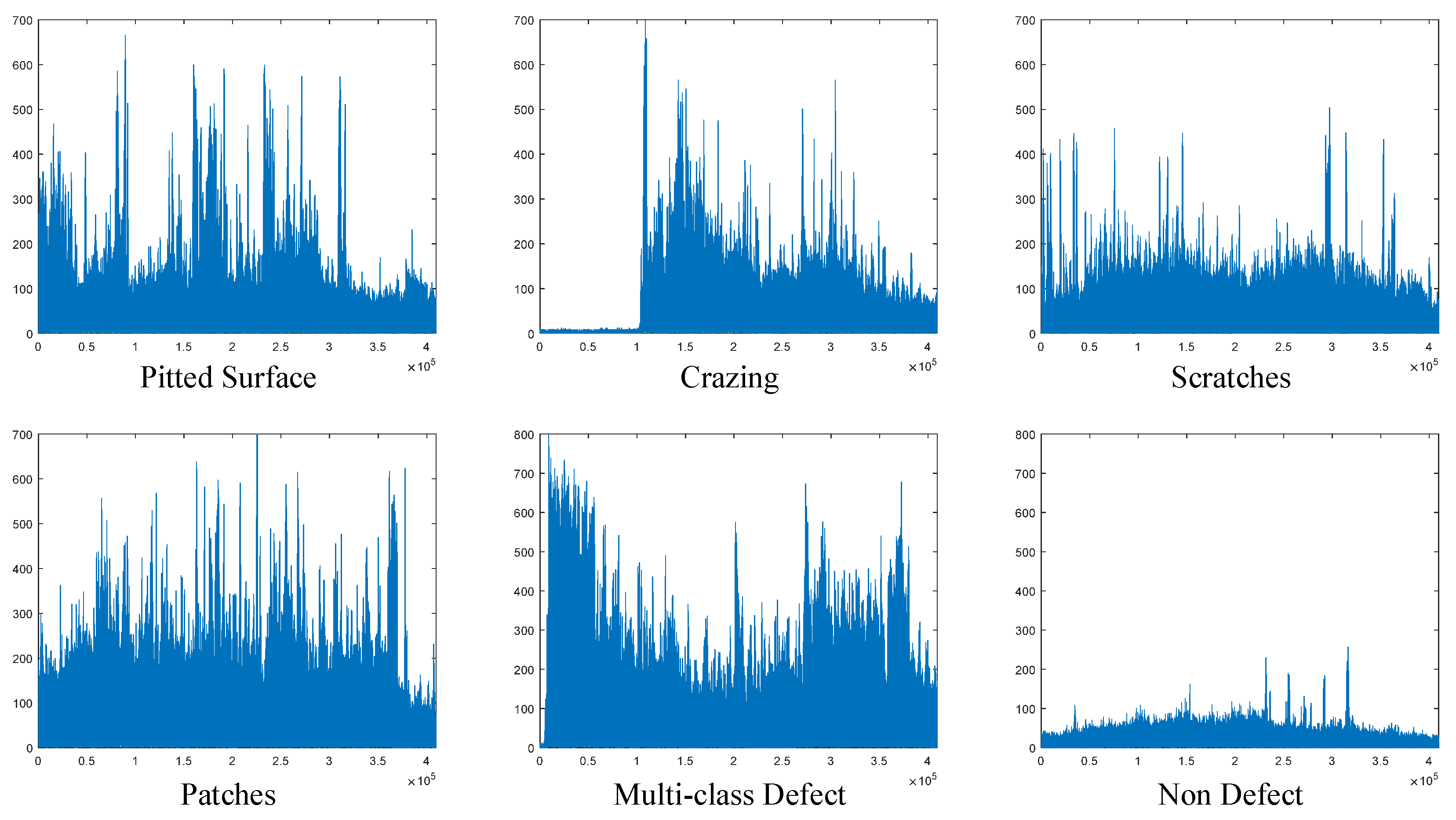
The graph showing the change in 1D stack data with the gradient applied for each class is presented in Figure 4. As observed in this figure, the gradient operation yields different amplitude values depending on the type of surface defect. Particularly in the non-defect class, the gradient output values are minimal, indicating little change across the dataset for this class.

In the final step, spectrogram images were generated from the 1D stack data. The Hamming window was selected for signal windowing due to its advantages, especially its narrow main lobe and rapidly decaying side lobes in the frequency domain. These features help prevent spectral leakage, which can weaken the accuracy of spectral information. A sample size of 512 was chosen for the window, and the overlapping ratio was set at 0.125. This overlap helps reduce data loss in the 1D stack, but it also increases the computational load required to produce the spectrogram images.

To enhance the clarity of the spectral data, special attention was given to amplitude values while generating the spectrogram images. A threshold was applied to filter out points with low amplitude values, as high-amplitude points are generally more reliable in terms of spectral information. This approach simplifies the images, which is beneficial when using neural network classifiers, as less complex images tend to improve the classification performance. A 512-point FFT length was applied to ensure consistency. The resulting spectrogram images for each class are displayed in Figure 5, where distinct patterns can be observed for each class, demonstrating the effectiveness of this approach for capturing class-specific spectral features. The colormap viridis option was selected for spectrogram coloring.

Using colormap options like viridis in spectrogram visualization offers several advantages. Viridis provides perceptual accuracy, as it is designed with evenly spaced color differences that allow users to distinguish variations in data more easily. It also maintains readability in monochrome formats, ensuring that important information is preserved even when printed or viewed in low-resolution settings. The smooth, linear color transitions of Viridis avoid abrupt shifts, making it easier to interpret differences in intensity or frequency. Additionally, Viridis ensures that small changes in data are accurately represented, reducing the risk of misinterpretation, which is particularly important for scientific visualizations.

As shown in Figure 5, there is sudden color darkening or sudden appearance and disappearance of color lines in all classes except the class with no error. This shows that the Viridis option is ideal for spectrogram transformation.

The convolution layer of the CNN method intends to extract characteristic features processing input samples with convolution filters [24]. The mathematical computing of two functions is described as convolution. By conducting element-wise multiplication on each element, the convolution computing in the CNN technique implements a filter or kernel function utilized for the raw data’s transformation into processed data [25,26]. Each window’s output in a shift operation is determined by the total multiplication of the element information [27,28].

The batch normalization (BN) technique is used to design a more regular convolutional neural network. Moreover, during training, the CNN extinction gradient becomes more resistant [29,30].

In the Rectified Linear Unit layer (ReLU), the full “f(k) = max(0, k)” formula is used for all inputs as the layer activation function [31,32]. ReLU’s derivative is more appropriate and performs faster for algorithms like backpropagation as it is simpler than the sigmoid function.

The softmax function is typically used for the output in deep learning models [33]. The function converts the class scores from the fully connected layer to probabilistic values ranging from 0 and 1. The softmax function is denoted by $S\left(a_j\right)$ in Equations (1) and (2). It obtains an N-dimensional input vector, then produces a subsequent input vector with N-dimensional, having values between 0 and 1 [34,35]. Additionally, even though the softmax function is frequently chosen for the output layer in deep learning models, an SVM classifier can be preferred [36]. The exponential feature of the softmax function makes the differences across classes more certain.

$$S\left(a_j\right):\left[\begin{array}{c}{a}_1\\ \dots .\\ a_n\end{array}\right]\to \left[\begin{array}{c}{s}_1\\ \dots .\\ s_n\end{array}\right]$$

(1)

$$S\left(a_j\right)={\displaystyle \frac{e^{a_j}}{{\sum }_{k=1}^n{e}^{a_k}}}$$

(2)

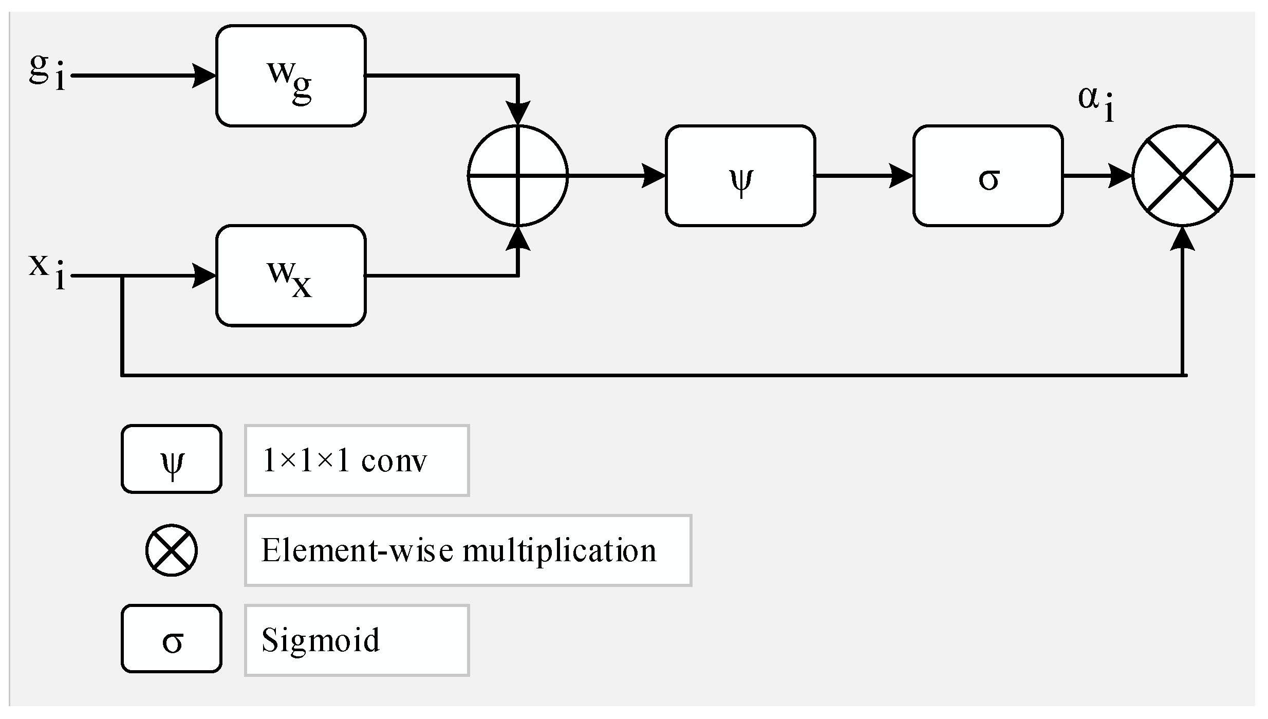
Figure 6 represents the attention module utilized in this research. The gating signal vector, symbolized by $g_{i }$, has a wider scale at the feature map of output for ith layer “($x_i$)”, determining the focus region for each pixel [37]. Equations (3) and (4) give a computed output by applying element-wise multiplication.

$$output={\alpha }_i\times x_i$$

(3)

$${\alpha }_i=\sigma ({\phi }^T\left({w_x}^T{x}_i+{w_g}^T{g}_i+b_g\right)+b_{\phi })$$

(4)

The linear transformations $w$ and $\phi$ using the 1 × 1 × 1 dimensional convolution operator are the bias terms $b_{\phi }$ and $b_g$, respectively. The weights of the attention modules are adjusted randomly at first when the entire deep architecture is trained from end to end [38].

In conventional neural networks, each layer provides information to the next layer. Each layer enhances the subsequent layer directly for the network having residual blocks, then advances to layers, which are two to three hops away [39]. In multi-layer networks, the gradient vanishing problem is decreased by residual blocks. The two significant points of residual blocks are given below.

-

The inclusion of new layers would not harm the model performance because regularization will disregard them if not necessary.

-

When incoming layers are convenient, layer weights or kernels are not “0” because of present regularization. Therefore, the model performance can slightly improve.

The training of the attention mechanism and the residual blocks were applied concurrently in parallel in the developed PARC model. The main target is to transfer feature maps in residual and attention structures into one feature map. Hence, during the training phase, optimization determines the characteristic values from every two structures obtained from the feature map.

7. INCA Algorithm

Increased system speed without reducing approach success is the most important aim of feature selection techniques. The literature on machine learning algorithms has been enhanced by several feature selection methods [40,41,42]. Specifically, the feature selection techniques reduce the computational cost of the deep learning algorithms having a lot of features. The performance of the feature selection approach on the feature set should be profoundly assessed [43]. However, in deep learning methods, the application of this analysis method is not time-saving. While the Minimum Redundancy Maximum Relevance (mRMR) technique performs better by using a non-parametric feature set, Principal Component Analysis and the Linear Discriminant analysis techniques outperform by applying a linear feature set [44]. For classification problems, current research mostly depends on feature extraction-based algorithms in terms of feature weight relations [45,46,47].

The NCA is one of the most popular features of importance-based selection algorithms since they offer a variety of classification strategies. Additionally, the computational time for these approaches outperforms the PCA and mRMR algorithms.

Neighborhood Component Analysis (NCA), a method for feature selection and dimensionality reduction that is widely used in classification studies, is one of the most reliable supervised learning approaches for classifying multidimensional data into distinct classes [48,49]. The classification tasks performed by NCA are carried out with learning vector optimization criteria related to the categorization accuracy performance of the nearest neighbor classifier. In particular, a linear projection chosen by NCA maximizes the projected area’s performance of the nearest neighbor classifier. In NCA, training data with related class labels are applied to choose the projection that divides the classes effectively in the detected area. Nevertheless, the NCA makes assumptions about the distribution of each class, which are not reliable. It offers an equivalent fit to Gaussian mixtures for distribution modeling. To maximize the objective function F(w) for w, the regularized objective function is used in Equation (5).

$$F\left(w\right)={\displaystyle \frac{1}{n}}{\sum }_{i=1}^n{P}_i-\mathsf{\lambda }$$

(5)

where the overall sample size is n, the value of the probability of ith the specimen is “P_i”, the parameter of regularization is “λ”, the dimension of the feature is “p” and the weight of the feature is “w_r”. The weight values for the feature may be very near to “0” in case the selection of “λ” is performed at random. The relevant features have no importance for the method when weights are very near to zero. Thus, the parameter λ has to be arranged.

Iterative Neighborhood Component Analysis (INCA) holds advantages over Neighborhood Component Analysis (NCA) primarily due to its adaptive feature selection mechanism. Unlike NCA, INCA iteratively selects features, allowing it to dynamically adjust and optimize the learning process by choosing the most relevant features for a given task. This adaptability enhances the discriminative power, robustness, and generalization performance. By reassessing and modifying feature selections during each iteration, INCA is better equipped to handle diverse datasets and mitigate the impact of noisy or irrelevant features. The flexibility offered by INCA in tailoring its approach to specific dataset characteristics makes it a promising choice for various machine learning applications.

Choosing the parameter λ randomly may not give the best feature selection result. Here, the most reliable way to select the lambda parameter is to use an optimization algorithm. The Stochastic Gradient Descent (SGD) algorithm provides exemplary performance in many optimization problems. In this study, the lambda parameter used in INCA was selected with the SGD optimization algorithm. The pseudocode expression of this algorithm (INCA) is given in Algorithm 1.

Algorithm 1. Pseudocode of the PARC model

Inputs: features from the PARC model, labels,

Output: the selected feature (features_out)

1: features_out = INCA_algorithm (features, labels)

2: begin

3: nca = fscnca (Xtrain, ytrain, ‘sgd’, bestlambda);

4:   for i = 1 to N do

5:      search the best lambda parameter by using the NCA

6:   end for i

7:   compute feature weights with the best lambda

8:   indeces = weights (indices)

9:      for j = 1 to length (features) do

10:         if weights (j) >= threshold

11:            append j to the new indices list

12:         end if

13:      end for j

14:   features_out = fea[new_indeces]

15:   return features_out

16: end

The parameter N is the number of optimization iterations and is set to 20 (default value). The threshold value is used to eliminate features including low-weight values. For the binary and multi-class classification, threshold values were selected as 0.5 and 0.2, respectively.

8. Experimental Studies

The computer used in the experimental studies has a 4 GB graphics card, i7 intel 5500U processor (Intel, Santa Clara, CA, USA), and 16 GB RAM, and the MATLAB 2021a program was installed on Windows 11 and used to code the suggested technique. Training the suggested Parallel Attention–Residual CNN (PARC) model was carried out for multi-class and binary classification at the first step of the suggested methodology. The epoch value was chosen as 100 to achieve maximum performance. This ensured sufficient training iterations. The mini-batch size was chosen as 32. This was the maximum allowed by the hardware for the PARC model used. The initial learning rate was chosen as 0.001. For smaller values, the training time increased and for larger values, the classification performance decreased. The SGDM technique was used as the optimization solver. The validation method employed was the 10-fold cross-validation, and the loss function was the cross-entropy. It took around 2 h to train the PARC model with the available hardware.

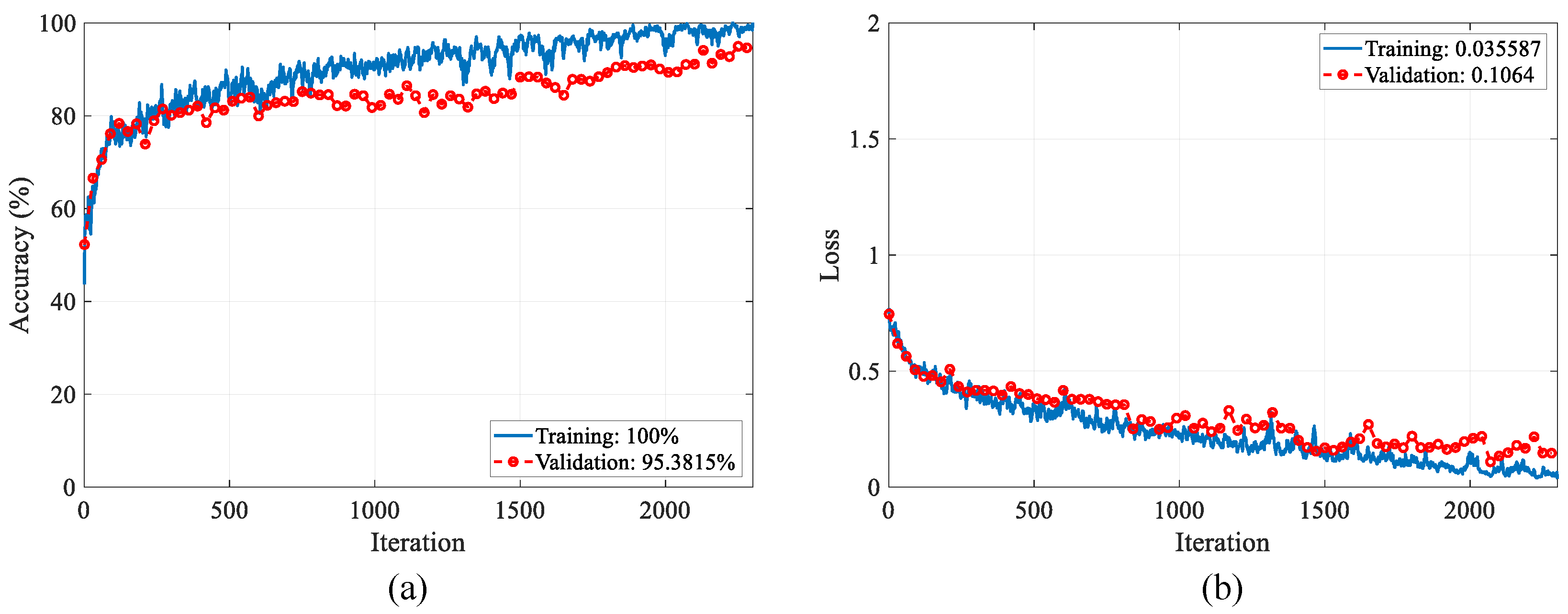
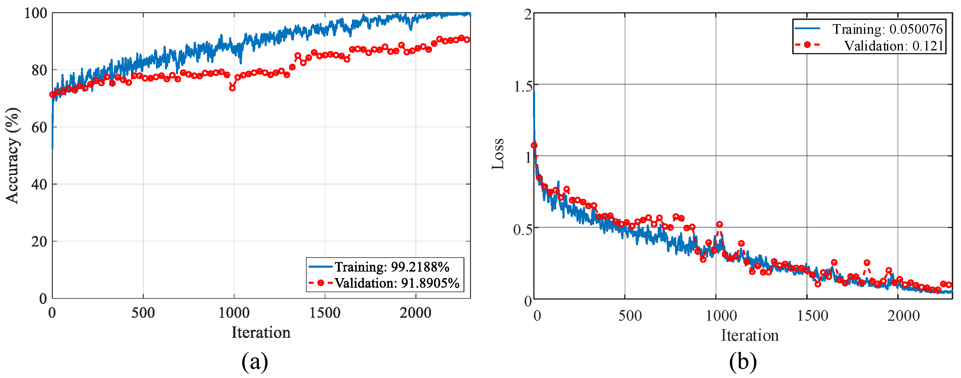
The loss values and accuracy graphics during optimization are presented in Figure 7 and Figure 8. The training–validation accuracy scores for the binary classification reached 100% and 95.38%, and the training–validation loss values reached 0.035 and 0.1, respectively. The training–validation accuracy scores for the multi-class classification reached 99.21% and 91.89%, and the training–validation loss values reached 0.15 and 0.12, respectively.

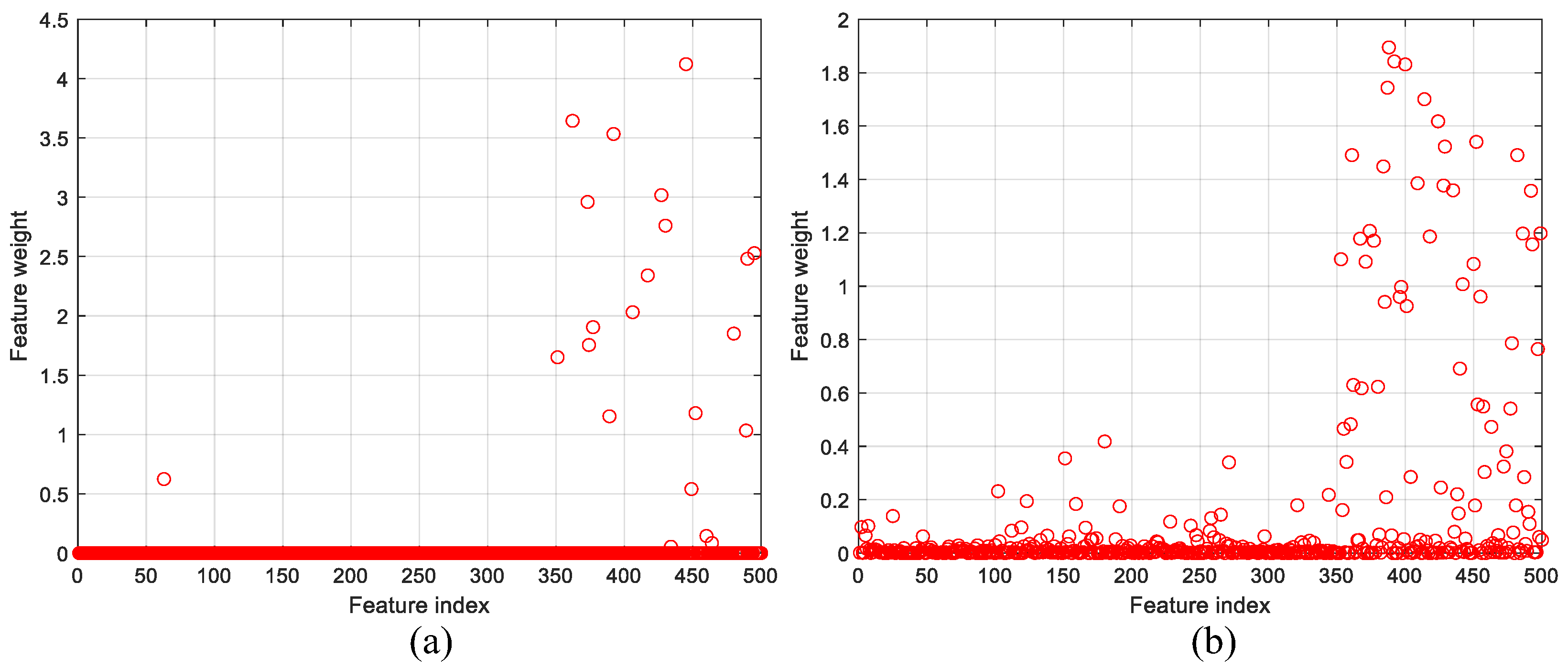
By using learnable parameters and input data, the extraction of five hundred deep features was performed by “fc4”, which is a fully connected layer in PARC. Therefore, the SVM algorithm could be used for the classification task instead of the softmax classifier. The Iterative Neighborhood Component Analysis (INCA) algorithm selected the most distinctive features and the computational cost decreased the execution time of the SVM classifier code. The number of the nearest neighbor (hyperparameter) was chosen as 10 (default value). Figure 9 shows the computed feature weights for each feature index. The threshold weights for the features to be selected with the INCA algorithm are set to 0.5 and 0.2 for binary and multi-class classification, respectively.

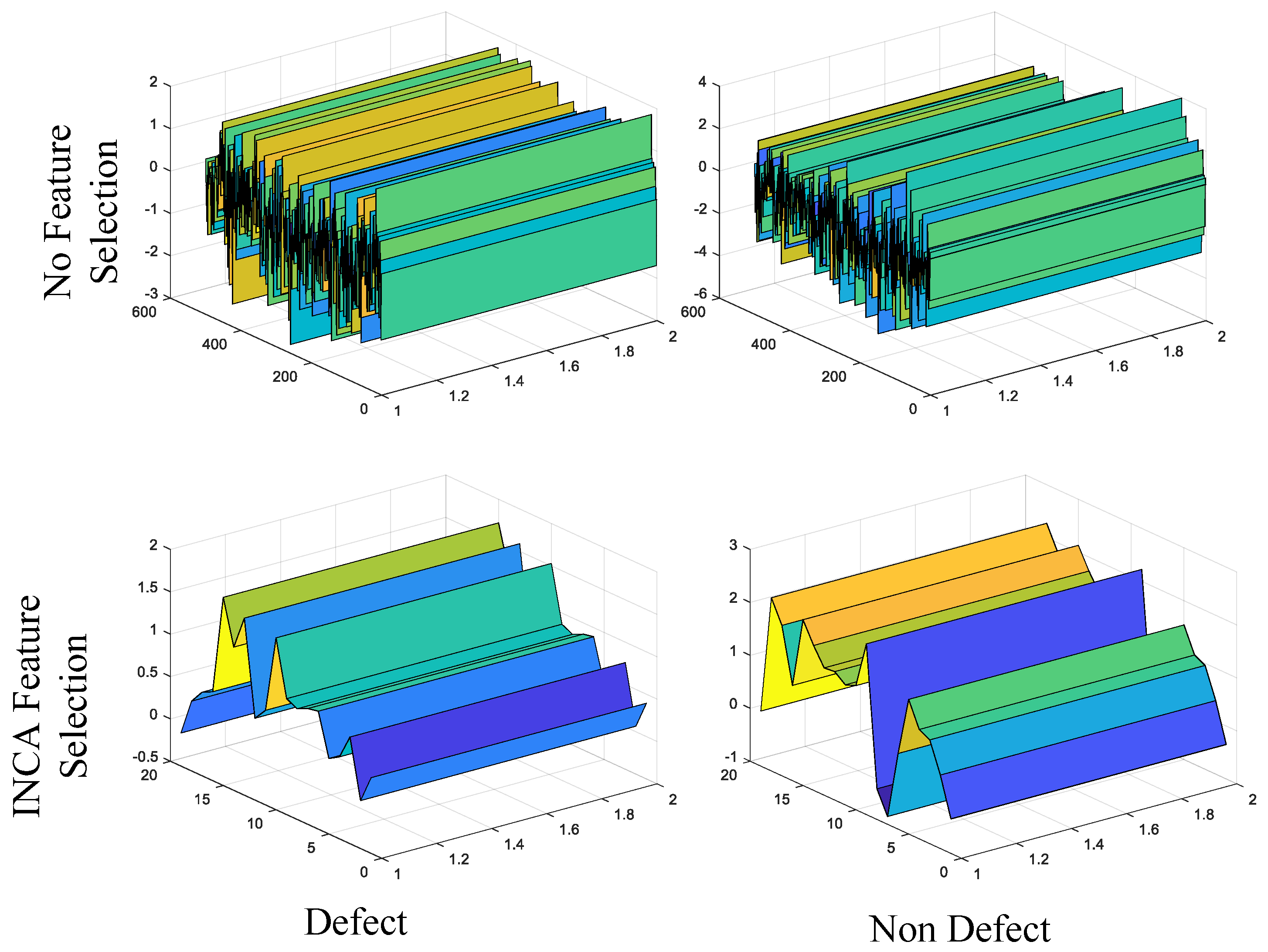
For binary and multi-class classification problems, 20 and 59 distinctive features were automatically selected by the INCA algorithm. Three-dimensional representations of the selected features are given in Figure 10 and Figure 11 for two classification problems. In Figure 10 and Figure 11, it is seen that the distinguishing characteristics of the features are increased with the feature selection process. In both figures, the rows represent classes and the columns show whether the feature selection process has been performed. The x-direction in the figures indicates the number of features. The y-direction provides the features’ amplitude values while the z-direction represents the feature depth. To show the features in three dimensions, this parameter has been added. For each display, it is set to 2.

The accuracy scores according to feature selection cases and different classifiers are given in

Table 1. Accuracy variations according to feature selection cases and different classifiers.

Classifier	No Feature Selection		INCA Feature Selection
	Binary	Multi–Class	Binary	Multi–Class
DT	90.2	88.7	91.3	90
SVM	95.4	94.6	98.3	97.5
KNN	92.5	93.1	95.1	94.9
NB	93.2	87.9	95.1	90
LD	92.8	93.5	94.1	95,2
SK	90.1	92.8	92.3	95.6
SD	88.7	93.6	90.1	95.4
RT	89.3	85.6	91.8	88.5

for two classification problems. DT, SVM, KNN, NB, LD, Subspace KNN (SK), Subspace Discriminate (SD), and RUSBoosted Trees (RT) were classifier algorithms in the Classification Learner (CL) tool in the Matlab program. The default hyperparameters were selected in the CL tool for the classification process. This ablation study was performed to evaluate the feature selection operation’s effectiveness and detect which classifier algorithm gave the best accuracy.

As seen in Table 1, the SVM with the Gaussian kernel provided the best accuracy for two classification problems. In the case without feature selection, for binary and multi-class classification problems, the accuracy scores were 95.4% and 94.6%, respectively. In the case of the INCA feature selection, for binary and multi-class classification problems, the accuracy scores were 98.3% and 97.5%, respectively. Subspace Discriminant and RUSBoosted Trees provided the worst accuracies for two classification problems. In multi-class classification and binary classification without feature selection, the worst performance of the accuracy rate was 88.7% (Subspace Discriminant) and 85.6% (RUSBoosted Trees), respectively. In multi-class classification and binary classification with the INCA feature selection, the worst performances of the accuracy rate were 90.1% (Subspace Discriminant) and 88.5% (RUSBoosted Trees), respectively.

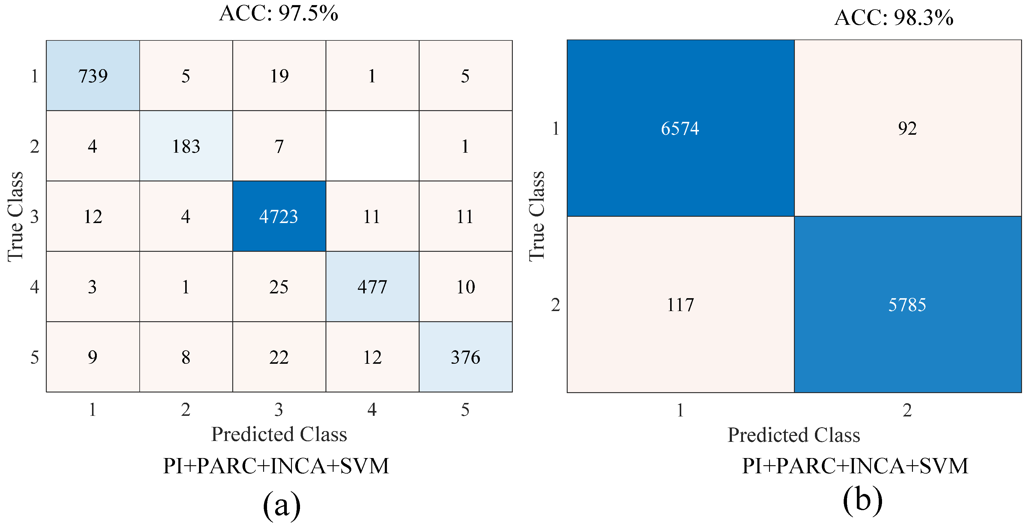
Figure 12 shows the confusion matrices of the proposed approach for the binary and multi-class classification tasks. In Figure 12a, the classes named 1, 2, 3, 4, and 5 represent the pitted surface, crazing, scratches, patches, and multi-class defect classes, respectively. In Figure 12b, the classes named 1, 2, 3, 4, and 5 represent the defect and non-defect classes, respectively. For the binary and multi-class classification problems, the accuracy scores were 98.3% and 97.5%, respectively.

Performance metrics, including the sensitivity (SN), specificity (SP), precision (PR), and F-score, were computed by using true positive (TP), true negative (TN), false positive (FP), and false negative (FN) values. The results of the computed metrics are given in

Table 2. Other performance metric results of the proposed approach for binary and multi-class classification.

Classification Mode	Classes	SN	SP	PR	F-Score
Binary	Defect	0.986	0.98	0.983	0.984
	Non-defect	0.98	0.986	0.984	0.982
Multi-Class	Pitted surfaces	0.961	0.995	0.963	0.962
	Crazing	0.938	0.997	0.91	0.924
	Scratches	0.992	0.96	0.985	0.988
	Patches	0.924	0.996	0.952	0.938
	Multi-class defects	0.881	0.996	0.933	0.906

.

For the binary classification, the SN, SP, PR, and F-score values of the defect class were 0.986, 0.98, 0.983, and 0.984, respectively. The SN, SP, PR, and F-score values of the non-defect class were 0.98, 0.986, 0.984, and 0.982, respectively. For the multi-class classification, the best SN (0.992), SP (0.996), PR (0.985), and F-score (0.988) values were obtained for the scratches, patches and multi-class defects, scratches, and scratches classes, respectively. The worst SN (0.881), SP (0.96), PR (0.985), and F-scores (0.988) values were obtained for the multi-class defects, scratches, crazing, and multi-class defect classes, respectively.

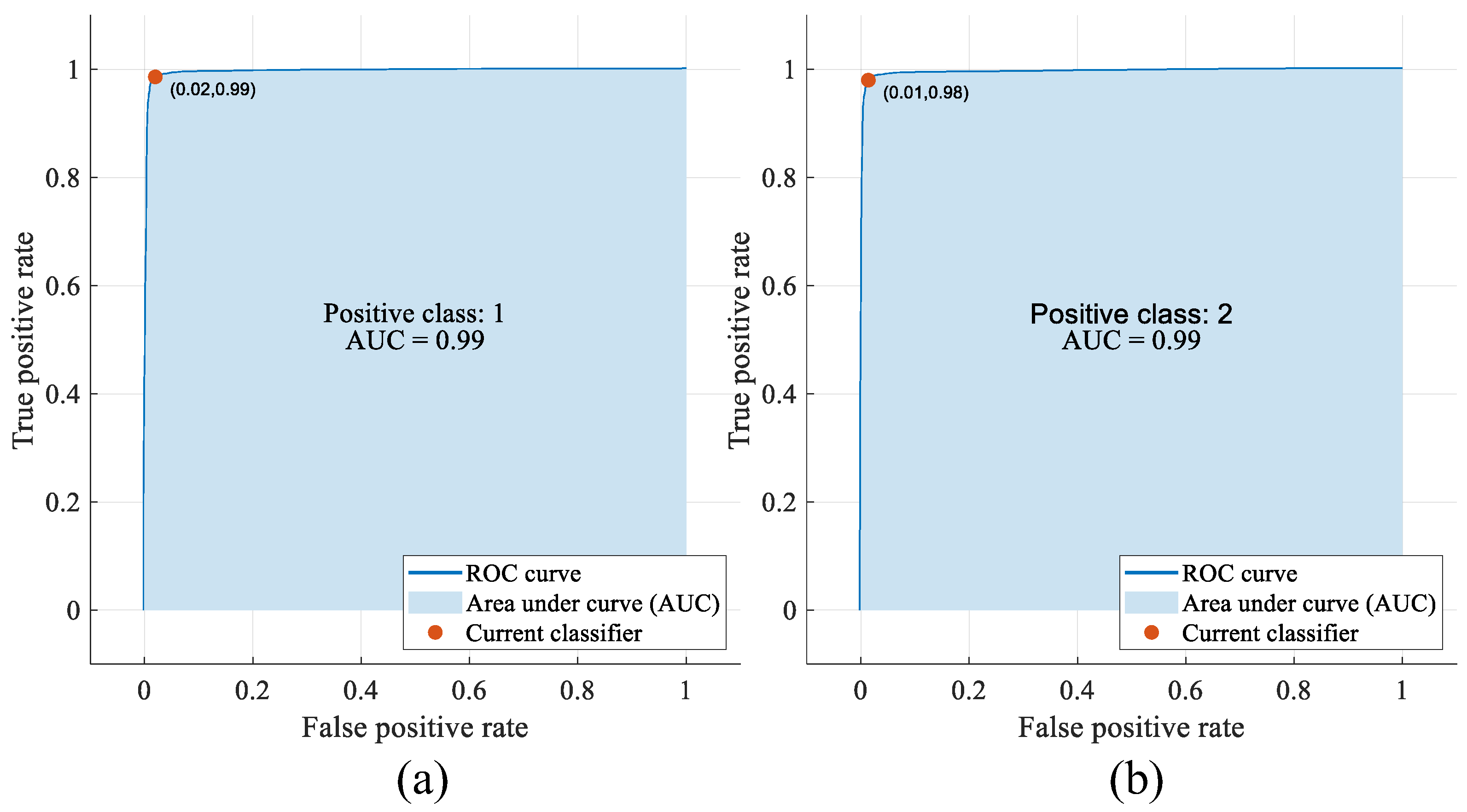
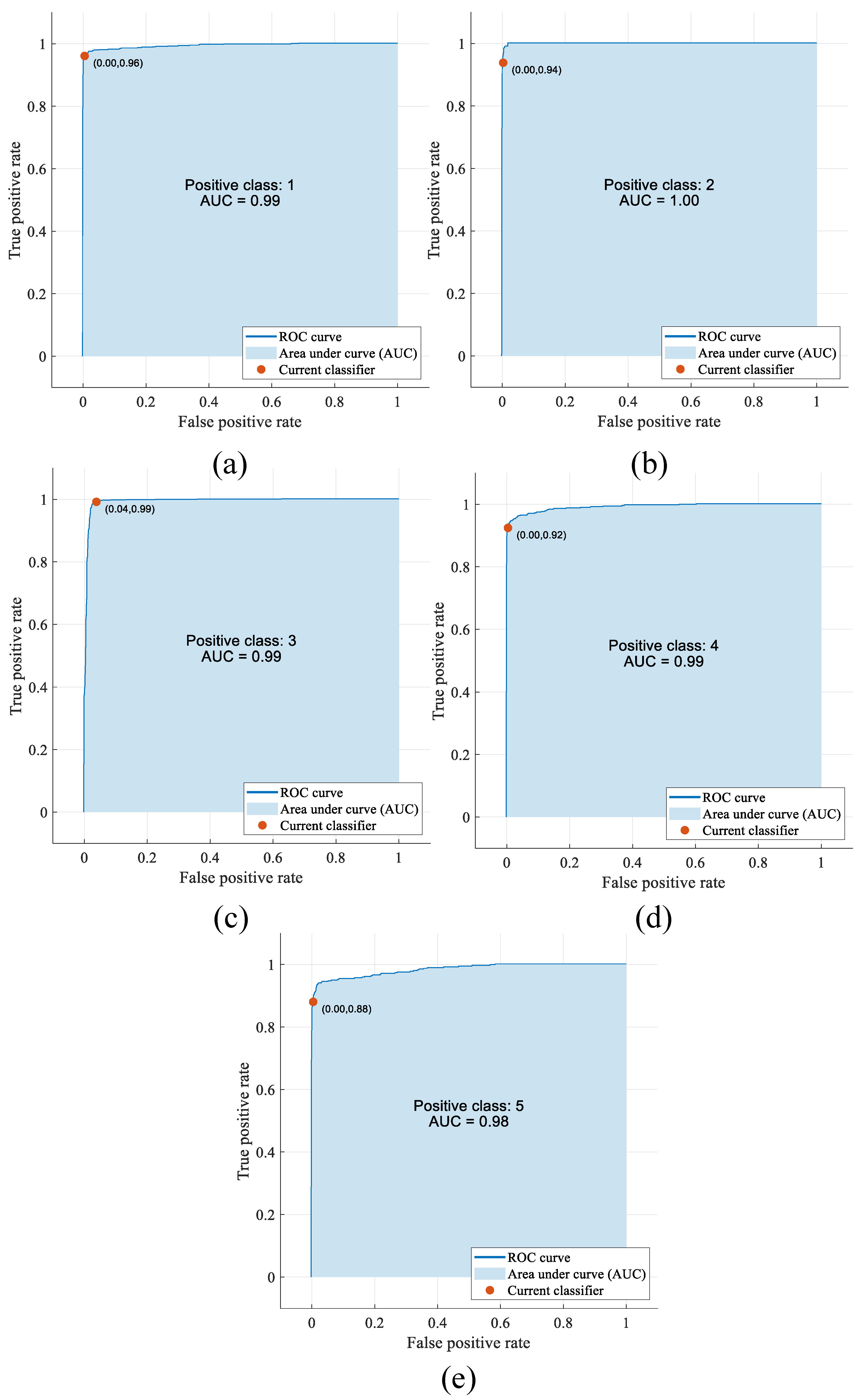
Figure 13 and Figure 14 show the ROC curves and AUC values for the two classification problems. In Figure 13, positive classes 1 and 2 include the defect and non-defect classes, respectively. In Figure 14, positive classes 1, 2, 3, 4, and 5 include pitted surfaces, crazing, scratches, patches, and the multi-class defect classes, respectively.

As seen in Figure 13a,b, the AUC values were 0.99 for positive classes 1 and 2. As seen in Figure 14a–e, the AUC values were 0.99, 1.00, 0.99, 0.99, and 0.98 for positive classes 1, 2, 3, 4, and 5, respectively.

9. Discussion

In this section, ablation studies for the proposed approach were performed and the proposed approach was compared with state-of-the-art methods. Figure 15 and Figure 16 show the effect of processed images (PI) and residual attention strategies on classification accuracy. Descriptive summary information about these ablation studies is provided in

Table 3. Summarizing information about the ablation study for the proposed approach ((a) binary classification, (b) multi-class classification).

Model Name	Model Info	Acc (a)	Acc (b)
RI + CNN	Raw images + PARC model without attention and residual structures	93.00%	87.20%
PI + CNN	Processed images + PARC model without attention and residual structures	93.50%	89.20%
PI + A-CNN	Processed images + PARC model without residual structures	93.90%	89.90%
PI + R-CNN	Processed images + PARC model without attention structures	94.50%	91.20%
PI + PARC	Processed images + PARC model (no feature selection with INCA and no SVM classifier)	95.40%	91.90%
PI + PARC + SVM	Processed images + PARC model +SVM (no feature selection with INCA)	96.80%	93.90%
PI + PARC + INCA + SVM	Proposed approach	98.30%	97.50%

for binary and multi-class classification, respectively.

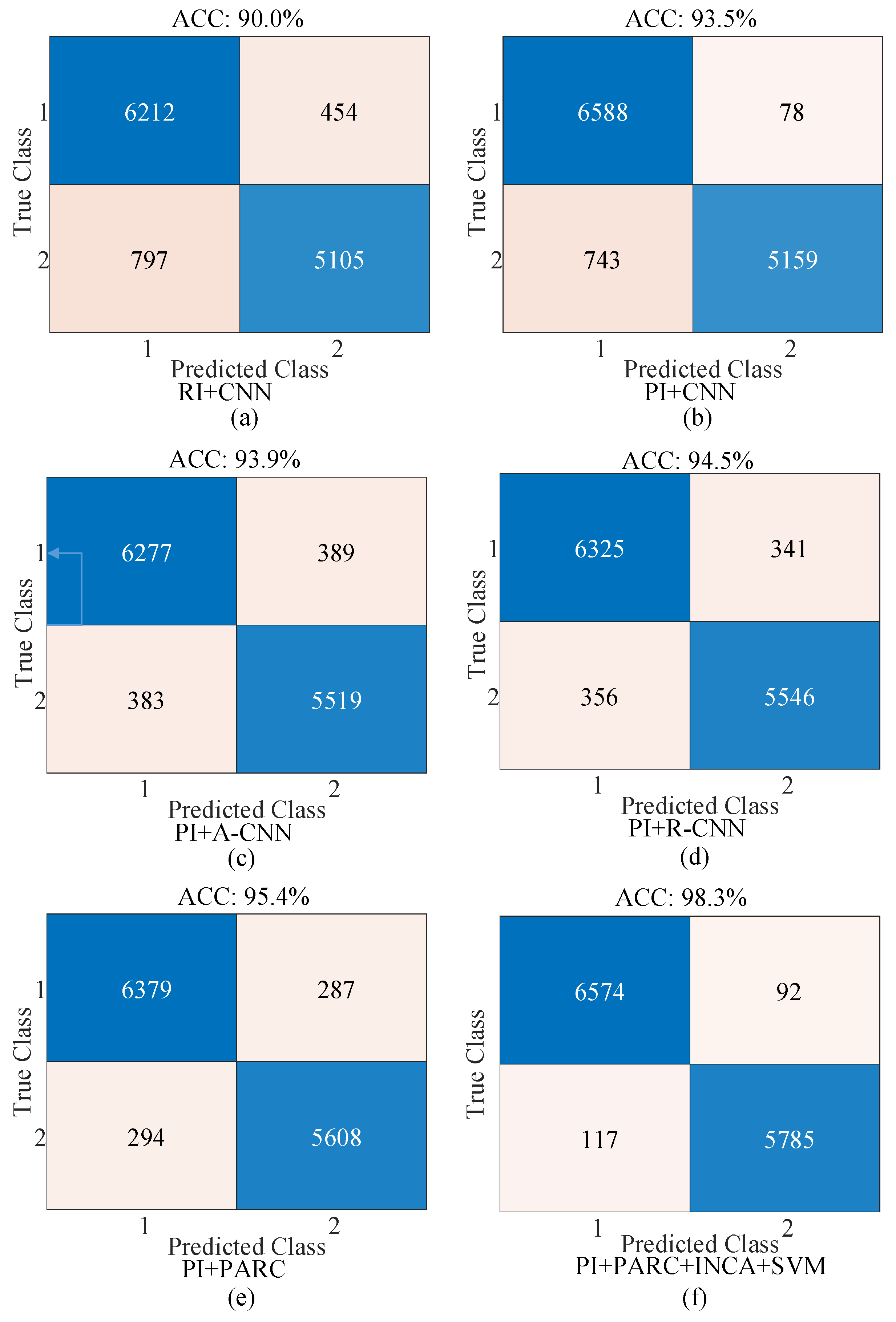
As seen in Figure 15 for the binary classification, the best accuracy was obtained by the proposed approach (PI + PARC + SVM) while the worst accuracy was obtained by the raw image (RI) + CNN strategy (Figure 15a). In Figure 15b, PI instead of RI was used for the classification and the classification accuracy was improved by 3.5%. In Figure 15c, the attention structure (PI + A-CNN) was added to the CNN model in Figure 15b. The classification accuracy was improved by 0.4%. In Figure 15d, the residual structure (PI + R-CNN) was added to the CNN model in Figure 15b. The classification accuracy was improved by 1.0%. In Figure 15e, the parallel residual and attention structure (PI + PARC) was added to the CNN model in Figure 15b. The classification accuracy was improved by 1.5%. In Figure 15f, the SVM classifier with INCA feature selection algorithm was applied in place of the softmax classifier in the proposed Parallel Attention–Residual CNN (PARC) model and the accuracy of classification was improved by 2.9% compared to the model in Figure 15e.

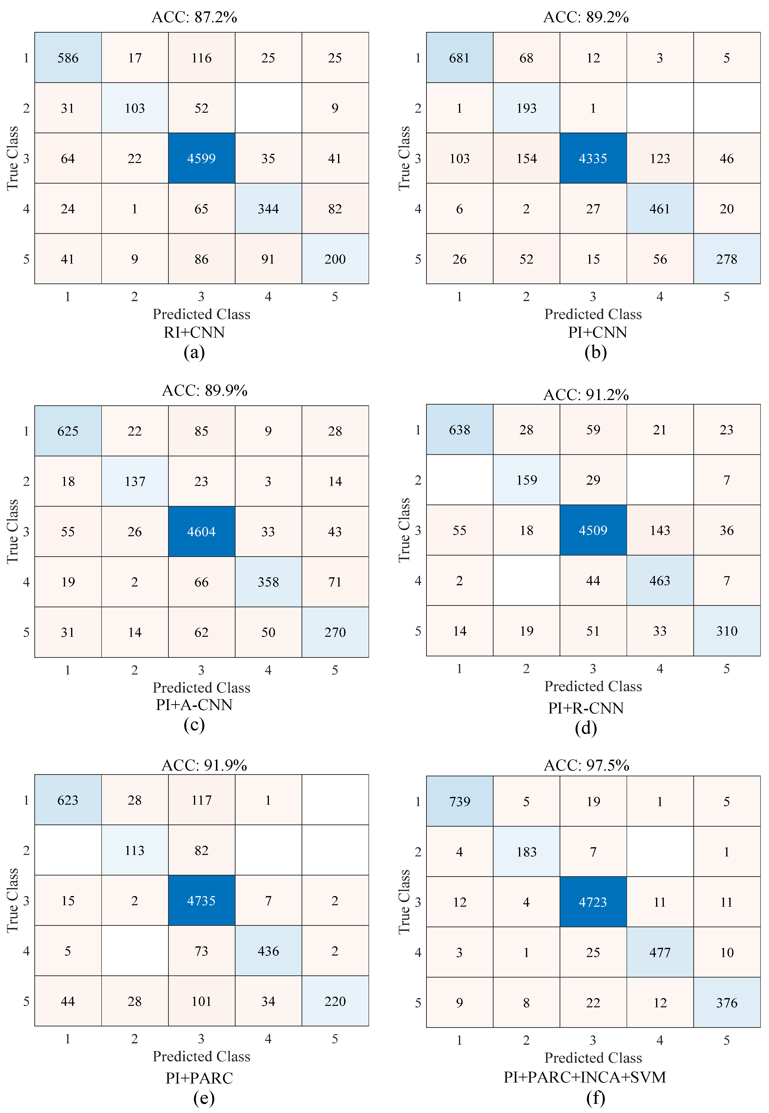
As seen in Figure 16 for the multi-class classification, the best accuracy was obtained by the proposed approach (PI + PARC + SVM) while the worst accuracy was obtained by the raw image (RI) + CNN strategy (Figure 16a). In Figure 16b, PI instead of RI was used for the classification, and the accuracy performance of classification was increased by 2.0%. In Figure 16c, attention structure (PI + A-CNN) was added to the CNN model in Figure 16b. The classification accuracy was improved by 0.7%. In Figure 16d, the residual structure (PI + R-CNN) was added to the CNN model in Figure 16b. The classification accuracy was improved by 2.0%. In Figure 16e, the parallel residual and attention structure (PI + PARC) was added to the CNN model in Figure 16b. The classification accuracy was improved by 2.7%. In Figure 16f, the SVM classifier with the INCA algorithm was used instead of the softmax classifier in the suggested PARC method, and the accuracy performance of classification was improved by 5.6% in comparison with the model in Figure 16e.

Table 4. The classification accuracies of studies and the proposed model using the same dataset.

Authors	Methodology	Accuracy (%)
		Binary	Multi-Class
Proposed model	PI + PARC + INCA + SVM	98.9	94.5
Wang et al. [21]	ResNet50 + Faster R-CNN	97.47	-
Guo et al. [51]	GAN model	96.8	-
Chigateri et al. [52]	Exception model	87.6	85.0
Hu et al. [53]	SEResNET50	94.0	87.5
Fadli et al. [50]	Transfer learning (Xception)	94.0	85.0

presents the performance results of the proposed approach and state-of-the-art models using the dataset named “Severstal: Steel Defect Detection”. Fadli and Herlistiono [50] used the Xception network, a pre-trained CNN model for automated steel surface classification. For the binary and multi-class classification, the classification accuracies were 94% and 85%, respectively. Guo et al. [51] performed automated surface steel detection with a specific GAN model. The binary class classification performance reached 96.80% accuracy. A hybrid approach with Faster R-CNN models and ResNet50 was proposed by Wang et al. [21]. The prediction values obtained from weight activations of the ResNet model were utilized for the thresholding operation. If the scores were less than 0.3, the steel samples were considered to be defect-free. If scores were larger than 0.3, the samples were described as defective. With this method, the binary classification accuracy was 97.47%. Additionally, four copies of each steel sample image from the dataset were created, along with new class labels, using this method. The dataset was therefore multiplied by four. Steel surface flaw classification was conducted by Chigateri et al. [52] using the Exception model. They achieved an accuracy of 88% for binary classification and the same accuracy of 88% for multiple classification. A combination of the ResNet model with the squeeze-and-excitation networks suggested by Hu et al. [53] produced an accuracy value of 87.5% for the two-class classification task and 94% for the four-class classification problem.

The efficacy of the proposed method was assessed by employing an alternate dataset, specifically the NEU Surface Defect Database [54]. Consequently, the dependability of the suggested approach was enhanced. This dataset comprised six distinct types of surface defects: crazing (class 1), inclusions (class 2), patches (class 3), pitted surfaces (class 4), rolled-in scales (class 5), and scratches (class 6). Through the utilization of 10-fold cross-validation, the dataset, consisting of a total of 1800 samples distributed evenly with 300 examples in each class, underwent evaluation. Within this dataset, the suggested technique demonstrated a classification accuracy of 99.77%, as depicted in the confusion matrix presented in Figure 17.

As can be seen from the results in Table 4 and

Table 5. The classification accuracies of studies and the proposed model using the NEU Surface Defect Database.

Author	Method	Accuracy (%)
Yeung et al. [54]	Fused Attention CNN model	89.3
Tian et al. [55]	SegNet + CNN	89.6
Yi et al. [56]	Deep CNN	99.05
Li et al. [14]	Transfer learning (ResNet)	99.0
Fu et al. [15]	Lightweight CNN	99.61
Proposed approach	PARC, NRMI, SVM	99.77

, the proposed model improved the classification performance compared to other models using the same dataset. However, given that the methods’ training parameters and training–evaluation methodology differ, this finding does not necessarily imply that the proposed strategy is better than the others.

Table 5 presents the performance results of the proposed approach and state-of-the-art models on the NEU Surface Defect Database. Yeung et al. [54] introduced a novel hybrid model, which underwent training from the ground up by incorporating the CNN architecture and five attention layers. The resultant CNN model, enriched with integrated attention, demonstrated an accuracy of 89.30%. Meanwhile, Tian et al. [55] employed the SegNet model to reconstruct and segment images of steel surfaces, and subsequent classification using a CNN model with an end-to-end learning approach yielded a success rate of 89.60%. Yi et al. [56] utilized a 14-layer CNN model featuring five convolutional layers, achieving an impressive classification accuracy of 99.05%. Li et al. [14] implemented a transfer learning system based on the ResNet model, attaining a classification accuracy of 99.00% with the ResNet CNN model. In another approach, Fu et al. [15] leveraged the SqueezeNet framework to construct a lightweight CNN model, incorporating a blur operation for raw photo processing, resulting in a remarkable success percentage of 99.61%.

The proposed approach outperformed the CNN, pre-trained CNN, R-CNN, transfer learning, and GAN models due to its novel and task-specific design. Key innovations included the use of a spectrogram algorithm in pre-processing, which transformed image data into a more detailed representation of surface defects, and the Parallel Attention–Residual CNN (PARC) model, which combined attention mechanisms for highlighting critical regions and residual connections for preserving important feature information. Unlike traditional models that relied on softmax for classification, this approach extracted deep features and evaluated them using multiple classifiers, with the SVM yielding the best results. Additionally, the INCA feature selection algorithm reduced the computational complexity while improving the classification accuracy. This tailored methodology enhanced defect detection by focusing on capturing subtle pixel variations and optimizing performance for the specific task.

Commonly used CNN models in both datasets include either pre-trained CNN models, such as ResNet, or lightly weighted CNN models. The network file sizes of the proposed PARC model and other popular pre-trained models with weights are given in

Table A2. Sizes of the PARC model and popular pre-trained CNN models.

CNN Model	Model File Size (MB)
ResNet	93.2
VGGNet	502.9
AlexNet	222.03
MobileNet	12.95
PARC Model	64.7

. The PARC model has less weight than the other pre-trained CNN models, except the MobileNet model. Therefore, the execution time is optimal for both training and testing. In addition, accurate classification is more important than speed in the detection of steel surface defects.

Table 6. Comparison of the proposed pre-processing method with basic image enhancement algorithms.

Method	Description	Multi-Class Accuracy (%)	Binary Accuracy (%)
Raw Images + CNN	Baseline method without any pre-processing.	93	87.2
Histogram Equalization + CNN	Enhances global contrast by redistributing image intensities.	93.4	88.7
Gamma Correction	Adjusts brightness using nonlinear intensity mapping.	93.2	87.9
CLAHE + CNN	Applies adaptive histogram equalization locally to improve contrast in homogeneous areas.	93.3	88.9
Unsharp Masking	Sharpens the image by emphasizing edges and details.	93	87.5
Log/Power-Law Transform	Enhances low-intensity pixels, useful for improving contrast in dark regions.	93.2	88.6

presents the classification accuracy results for both multi-class and binary classification tasks using various image enhancement techniques followed by CNN-based classification. The proposed spectrogram-based method shows superior performance in both scenarios.

The experimental results demonstrate the effectiveness of the proposed spectrogram-based method in enhancing the discriminability of surface defects for both multi-class and binary classification tasks. While the baseline approach using raw images with CNN achieved a 93.0% accuracy for multi-class and 87.2% for binary classification, applying conventional image enhancement techniques such as histogram equalization, gamma correction, CLAHE, unsharp masking, and log/power-law transforms led to modest improvements. Among these, CLAHE and histogram equalization performed relatively better due to their ability to improve the local and global contrast, respectively. However, the proposed method outperformed all the others, achieving the highest classification accuracy of 93.5% in the multi-class scenario and 89.2% in binary classification.

This superior performance can be attributed to the spectrogram’s ability to transform gradient-derived signals into the time–frequency domain, enabling the capture of both spatial patterns and frequency-based features related to surface defects. Unlike conventional techniques that primarily operate in the spatial domain and focus on intensity or contrast, the spectrogram representation provides a richer and more informative input to the CNN by highlighting subtle defect structures. These results quantitatively validate the advantage of the proposed method over traditional enhancement techniques in terms of feature extraction and defect classification performance.

10. Conclusions

This study focuses on the automatic detection of surface defects, which is an important issue in steel fabrication. It has been made to increase the automatic classification performance with a specific deep learning-based strategy. The classification performance is enhanced by processed images and feature extraction in the Parallel Attention–Residual CNN (PARC) model. The PARC model outperformed the CNN model (no residual and attention structures), the R-CNN (Residual-CNN), and the A-CNN (Attention-CNN) models. In addition, the Iterative Neighborhood Component Analysis (INCA) algorithm efficiently reduced the size of the feature set and improved the classification performance for both datasets. The classification performance values obtained for the Severstal Dataset (SD) and the Neu-Surface Dataset (NSD) are summarized in

Table 7. Summary of the experimental results of the proposed method.

Criteria	SD 2-Class	SD 4-Class	NSD
Accuracy (%)	98.9	94.5	99.7
Sensitivity	0.98	0.94	0.99
Specificity	0.98	0.98	0.99
Precision	0.98	0.94	0.98
F-score	0.98	0.94	0.98
Performance improvement (%)	1.43	7.0	0.16

. As can be seen from Table 7, both datasets achieved 0.94 and above in all the performance metrics. In both datasets, the classification accuracy was improved according to the model that achieves the best performance out of the existing models. The classification performance is improved by 1.43%, 7.0%, and 0.16% for SD 2-class, SD 4-class, and NSD, respectively.

The good classification performance of the proposed approach makes it possible to use it for the real-time detection of steel surface defects. In the next phase, the recorded weights of the proposed approach can be tested on an artificial intelligence development kit such as an NVIDIA Jetson Orin Nano (NVIDIA, Santa Clara, CA, USA). Thus, once the test performance of the model is confirmed, it can be used in enterprises.

The most important limitation of the proposed model is that it is difficult to implement in real-time embedded systems due to the size of the model. This limitation can be solved with server-based systems. However, this may increase the financial cost.