Complementary Filter Optimal Tuning Methodology for Low-Cost Attitude and Heading Reference Systems with Statistical Analysis of Output Signal

Abstract

Complementary filters are commonly used in low-cost AHRS systems. This article presents an algorithm for selecting the time constant of a complementary filter for AHRS systems. The AHRS and complementary filtering principles of operation are described, followed by a methodology for calibrating the filter. A simple method for acquiring calibration data is introduced, and these data are subsequently used in the proposed iterative algorithm for optimal time constant selection. The described method minimizes measurement errors and improves the accuracy of the system, ensuring operational stability. For the synthesis, data are recorded in a static position of the system at various pitch and roll angles. Next, the optimal time constant of the complementary filter is determined. The statistical properties of the attitude angles are then analyzed. The proposed methodology for system assessment and analysis is discussed.

1. Introduction

Attitude and heading measurements are among the most important measurements on board various types of aircraft. In modern solutions, these are measured by an Attitude and Heading Reference System (AHRS). A typical AHRS consists of angular rate sensors, accelerometers, and magnetic heading sensors. The attitude and heading calculations are primarily based on angular rate sensors; however, due to their low-frequency errors (bias), correction is necessary, especially in low-cost systems. By low-cost systems, we refer to systems that use off-the-shelf MEMS (Micro-Electro-Mechanical-System) sensors, with a limited number of microcontrollers and other components that contribute to the overall cost of the system. MEMS sensors are used because of not only their low price but also their small size, which is crucial for small unmanned aerial vehicles (UAVs).

In recent years, the market for small UAVs has grown rapidly, particularly in military applications. In the area of measurement, control, and navigation, researchers have developed control algorithms for single aircraft [1,2], formation and swarm control algorithms [3], and navigation and measurement systems [4,5]. Also, solving problems with reliability is crucial [6,7]. Many small UAVs are designed as single-use weapons, meaning that solutions applied to them should be low-cost. The cost of the AHRS system influences the quality of sensors and the class of microcontroller used, which, in turn, affects the overall cost of the system. Although the second problem is less critical in several applications due to the development of high-efficiency microcontrollers, it should still be considered, particularly in the areas mentioned and similar ones. Higher computing resources increase the cost of the system and require more energy for operation. This aspect should also be considered in modern design trends. The algorithms applied should be as simple as possible to make the system more efficient.

Several researchers have focused on the problems of AHRS design, with the key issue being the proper functioning of the correction system. In general, three algorithms are used: the complementary filter, Kalman filter [8], and Madgwick filter [9]. The Kalman filter [10] minimizes the estimate error variance and is commonly used. Extended Kalman filters and unscented Kalman filters are solutions that can be applied in AHRS systems. However, their disadvantage is the high computational resources they require. The complementary filter [11] is the second solution, enabling very simple correction, and due to its simplicity, it is still used in low-cost systems, e.g., [12,13]. The third algorithm, the Madgwick filter, is gaining popularity, and it uses a gradient descent algorithm tailored to attitude estimation with quaternion algebra.

Among the three algorithms mentioned, the complementary filter is the simplest. It enables accurate attitude correction and does not significantly burden the microcontroller resources. Due to its simplicity, the complementary filter appears to be a very good option. An important task is developing a methodology for tuning the complementary filter and analyzing the properties of the acquired signal.

Several authors have studied the complementary filter for AHRS systems. Some researchers present results of complementary filter implementations in AHRS systems [8,14,15,16,17]; however, they do not present a direct methodology for filter synthesis. There is also research focused on the application of different forms of complementary filters. For example, Ref. [18] presents the design and implementation of an AHRS based on MEMS sensors and complementary filtering. They provide application details and results, but do not describe the tuning process in detail. The influence of the controller structure on the correction branch from the accelerometer to the static accuracy of the complementary filter is examined in [19].

The proposition of a novel complementary filter for micro-aircraft vehicles that is quaternion-based is presented in [20]. This filter enables quaternion correction using acceleration and magnetometer data. An advantage of this solution is the introduction of adaptive filter gain, which depends on the vehicle’s motion. However, details of the methodology for parameter tuning are not provided. Meyer et al. [21] propose a robust dynamic-state detection algorithm for use with aircraft state filters using an accelerometer as a vector measurement.

Complementary filter tuning is often performed using frequency-based methods, such as that shown in [22,23]. In [24], the $H_{\infty }$ method is used to shape complementary filters. A fuzzy logic system for tuning complementary filters is used in [25]. The mentioned methods are useful during AHRS synthesis; however, they do not minimize measurement error.

This article proposes a methodology for the optimal selection of complementary filter parameters. This topic was found to be important based on the authors’ experience in designing several aeronautical control and measurement systems [7,14,22,26,27,28,29,30]. Pitch and roll channels are described. The tuning is based on signals recorded during static tests, which allows for the efficient synthesis of AHRS systems and other systems involving signal correction. These methods can be implemented for low-cost solutions without the need for sophisticated equipment. This approach will significantly improve measurement quality. Additionally, the statistical properties of the example results are discussed. This article is structured as follows: First, the principles of AHRS operation are described, along with the required accuracy. Next, the methodology for filter calibration is presented and the statistical properties of the signal received are discussed. Finally, a discussion is presented and future work is proposed.

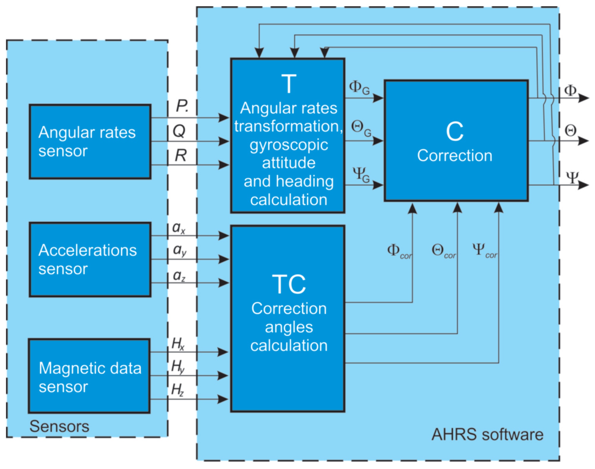
2. AHRS Principles of Operation

Figure 1 presents a general scheme of a typical AHRS.

Angular rates $P,Q,R$ in the body frame $F_b$ are measured by rate sensors. To calculate the attitude angles and heading, these rates need to be transformed to the $F_v$ frame [31]. The $F_v$ frame is parallel to the Earth frame, with its origin at the same point as the body frame $F_b$. Two algorithms can be used for the transformation. The first is the Tait–Bryan algorithm [31,32], which assumes three rotations around known axes. Equation (1) presents the transformation algorithm.

$$\dot{\overline{\Phi }}=L_{VB}\times {\overline{\Omega }}_K$$

(1)

where

$$\overline{\Phi }=\left[\begin{array}{c}\Phi \\ \Theta \\ \Psi \end{array}\right]$$

(2)

represents Euler angles in the Earth frame $F_V$ (roll, pitch, and yaw angles);

$${\overline{\Omega }}_K=\left[\begin{array}{c}P\\ Q\\ R\end{array}\right]$$

(3)

represents angular rates in the body frame $F_B$ (roll rate, pitch rate, yaw rate); and

$$L_{VB}=\left[\begin{array}{ccc}1& sin\Phi tan\Theta & cos\Phi tan\Theta \\ 0& cos\Phi & -sin\Phi \\ 0& {\displaystyle \frac{sin\Phi }{cos\Theta }}& {\displaystyle \frac{cos\Phi }{cos\Theta }}\end{array}\right]$$

(4)

represents the angular rate transformation matrix from $F_B$ to $F_V$.

A well known disadvantage of the presented algorithm is the discontinuity for a pitch angle of 90 degrees. To eliminate this inconvenience, an algorithm based on quaternion algebra is used [31,32]. It assumes one rotation around a known axis. The relationship between the quaternion derivative and angular rates measured in the body frame $F_B$ is as follows:

$$ϵ={\displaystyle \frac{1}{2}}{L}_e\times {\overline{\Omega }}_K$$

(5)

where

$$ϵ=\left[\begin{array}{c}{e}_0\\ e_1\\ e_2\\ e_3\end{array}\right]$$

(6)

represents the quaternion

$$L_e=\left[\begin{array}{ccc}-e_1& -e_2& e_3\\ e_0& -e_3& e_2\\ e_3& e_0& -e_1\\ -e_2& e_1& e_0\end{array}\right]$$

(7)

A quaternion can be obtained from the attitude and heading:

$$e_0=cos{\displaystyle \frac{\Phi }{2}}cos{\displaystyle \frac{\Theta }{2}}cos{\displaystyle \frac{\Psi }{2}}+sin{\displaystyle \frac{\Phi }{2}}sin{\displaystyle \frac{\Theta }{2}}sin{\displaystyle \frac{\Psi }{2}}$$

(8)

$$e_1=sin{\displaystyle \frac{\Phi }{2}}cos{\displaystyle \frac{\Theta }{2}}cos{\displaystyle \frac{\Psi }{2}}-cos{\displaystyle \frac{\Phi }{2}}sin{\displaystyle \frac{\Theta }{2}}sin{\displaystyle \frac{\Psi }{2}}$$

(9)

$$e_2=cos{\displaystyle \frac{\Phi }{2}}sin{\displaystyle \frac{\Theta }{2}}cos{\displaystyle \frac{\Psi }{2}}+sin{\displaystyle \frac{\Phi }{2}}cos{\displaystyle \frac{\Theta }{2}}sin{\displaystyle \frac{\Psi }{2}}$$

(10)

$$e_3=cos{\displaystyle \frac{\Phi }{2}}cos{\displaystyle \frac{\Theta }{2}}sin{\displaystyle \frac{\Psi }{2}}-sin{\displaystyle \frac{\Phi }{2}}sin{\displaystyle \frac{\Theta }{2}}cos{\displaystyle \frac{\Psi }{2}}$$

(11)

The attitude and heading can be calculated from the quaternion:

$$tan\Phi ={\displaystyle \frac{2e_0{e}_1+e_3{e}_2}{e_0^2-e_1^2-3_2^2+e_3^2}}$$

(12)

$$sin\Theta =2(e_0{e}_2-e_3{e}_1)$$

(13)

$$tan\Psi ={\displaystyle \frac{2e_0{e}_3+e_1{e}_2}{e_0^2-e_1^2-3_2^2+e_3^2}}$$

(14)

The correction angles in the block of correction angle calculation are determined using a geometric relationship.

An important task for ensuring the proper behavior of the AHRS system is the achievement of a correction. As mentioned in the introduction, several different solutions can be implemented. For the purposes of this article, a complementary filter was applied to correct the attitude and heading. Figure 2 presents a general scheme of a measurement system with a complementary filter.

Signal 1 and Signal 2 represent the same physical value; however, they are affected by different errors. Signal 1 is affected by a low-frequency error, which grows over time. Signal 2 is affected by noise. The errors typical for both signals are filtered by high-pass (for Signal 1) and low-pass (for Signal 2) filters. For proper measurement, the sum of the transfer functions must be equal to 1. Figure 3 presents a scheme of the complementary filter for the AHRS system.

Signal $\dot{X}$ is an angular rate measured by angular rate sensors and transformed to the frame $F_v$. Similarly, the $X_{\mathrm{COR}}$ signal is the correction signal calculated in the TC correction angle calculation block shown in Figure 1.

It should be noted that correction is improper in dynamic states; therefore, other correction signals should be considered, or correction should be turned off [11,14,33]. If a correction switching system has not been implemented, it would be impossible to use the AHRS on board an aircraft. An important task for ensuring correction quality is the analysis of static conditions.

The presented form of the complementary filter is easy to implement in low-cost systems and is sufficient for ensuring the proper behavior of the system as a whole. The proper value of the complementary filter determines the quality of the estimated signal, and the methodology for its tuning will be shown below.

The required accuracy of AHRS signals depends on several factors, such as the type of aircraft, its mission, and the control scenario. In [34], the required attitude measurement error is defined as 0.5% of the measurement range.

3. Methodology of Complementary Filter Calibration

Finding the optimal time constant for a complementary filter processing signals from a gyroscope and other sensors, such as accelerometers, using mathematical modeling methods is an extremely difficult task. This system works iteratively, which significantly complicates the analysis and evaluation of solutions to stochastic differential equations. Developing a model that also takes into account the variability of various parameters, including the technical specifications of gyroscopes and accelerometers, is an impossible task. Simplifying the theoretical model and/or idealizing the input signal undermines accurate error assessment and control.

In this situation, the most effective approach to optimizing this system is to implement numerical and statistical analyses. This was implemented in the R environment. This method allowed us to select a time constant for the complementary filter that minimizes errors, eliminates residual systematic errors, and improves the accuracy of the system orientation and ensures operational stability.

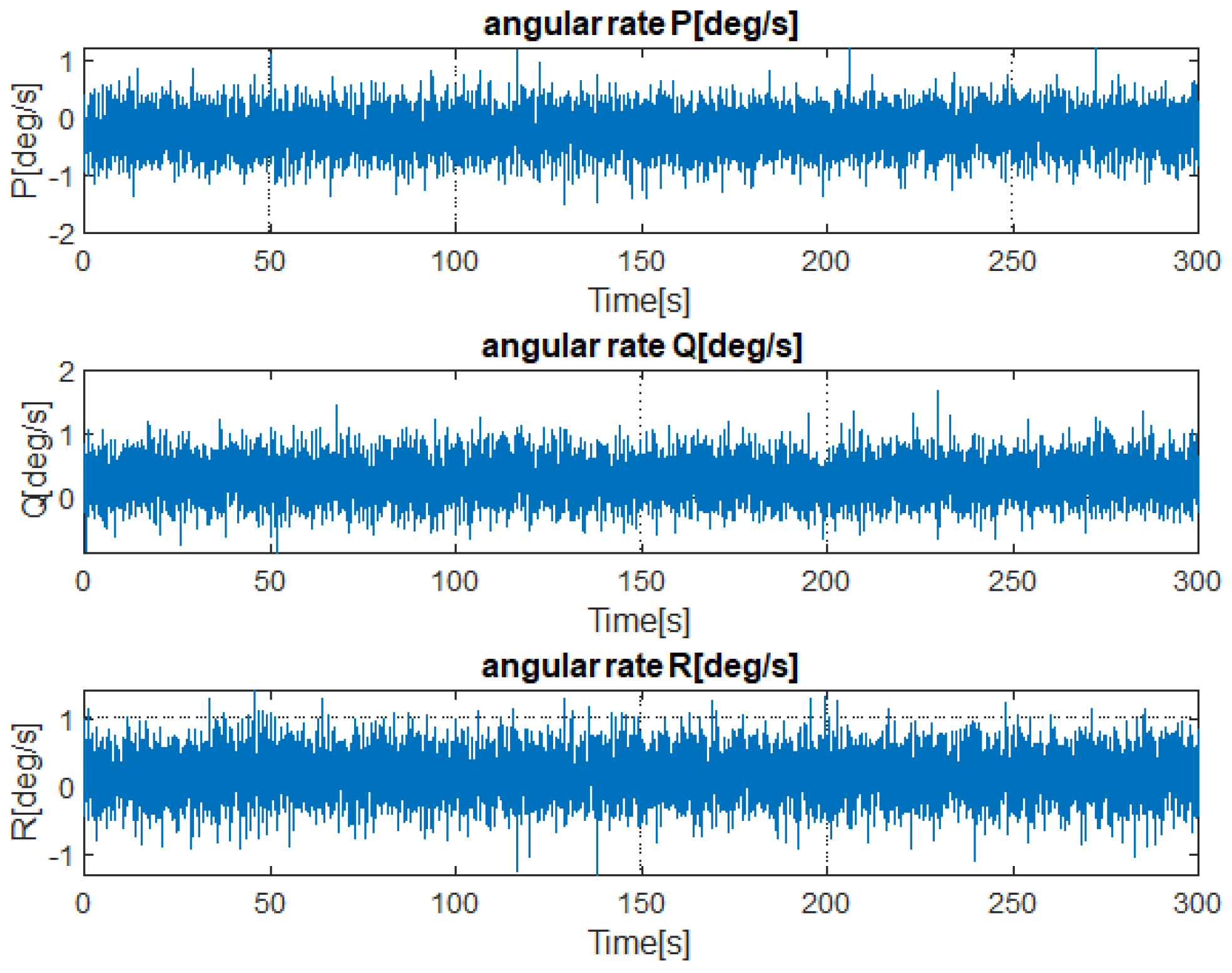
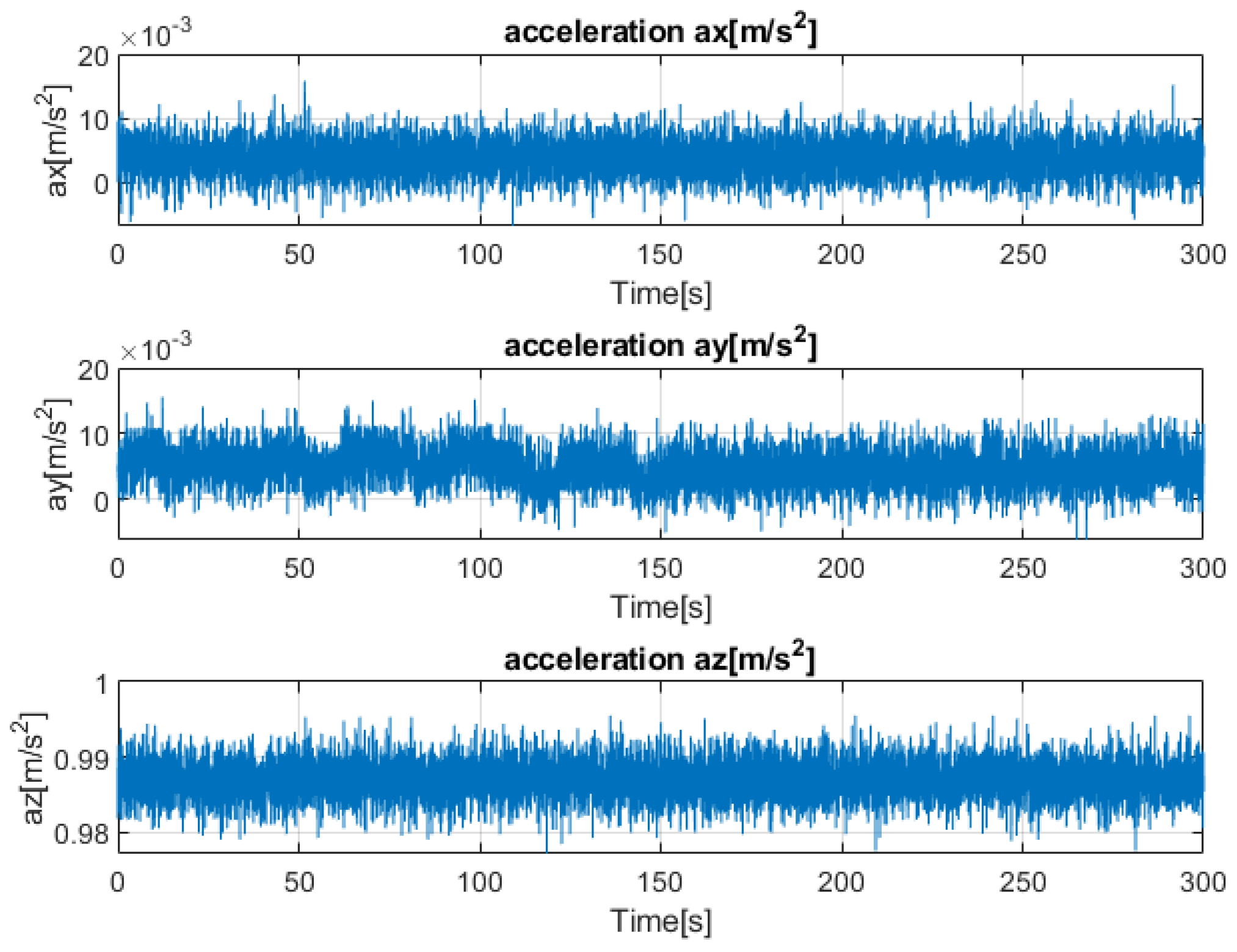
3.1. Data Collection

The first step was data recording in a static position of the system, at various pitch and roll angles. The following attitude angle values were chosen for both channels: 0, 5, 10, 15, 20, 25, and 30 degrees. Fourteen data sets were recorded, each corresponding to a specific attitude angle. The duration of each experiment was 300 s, and the data transmission frequency was 50 Hz (every 0.02 s). There were registered acceleration signals, $a_x$, $a_y$, and $a_z$, as well as angular rates, P, Q, R. For each angle, a set of 105,000 data points was recorded during each experiment, resulting in a total of 1,470,000 data points. Subsequently, the data were introduced into a simulation system in Matlab Simulink, where a model of the AHRS system with complementary filters was implemented. For each experiment, a set of attitude and heading angles was calculated, containing 45,000 additional data points for each analyzed angle and individual time constant. A total of 126 different time constant values were simulated for each attitude, which means 1764 simulation experiments for data acquisition. In total, there were 264,600,000 analyzed attitude data points. The experiments were conducted under controlled conditions to ensure objectivity and repeatability. Data acquisition was fully automated, and all recorded measurements were verified for consistency. The angular rates and acceleration data were obtained using an inertial measurement unit (IMU) and processed according to a predefined procedure. The determined attitude data were used to select the optimal time constant value for the complementary filter. Figure 4, Figure 5 and Figure 6 show example time series of the obtained data.

Figure 6 shows influence of the complementary filter time constant for the calculated angle. The results obtained show the possibility, and even the need, to select the time constant using a specific optimal criterion or based on the frequency analysis of the signal. Below, the methodology for selecting the optimal time constant will be presented.

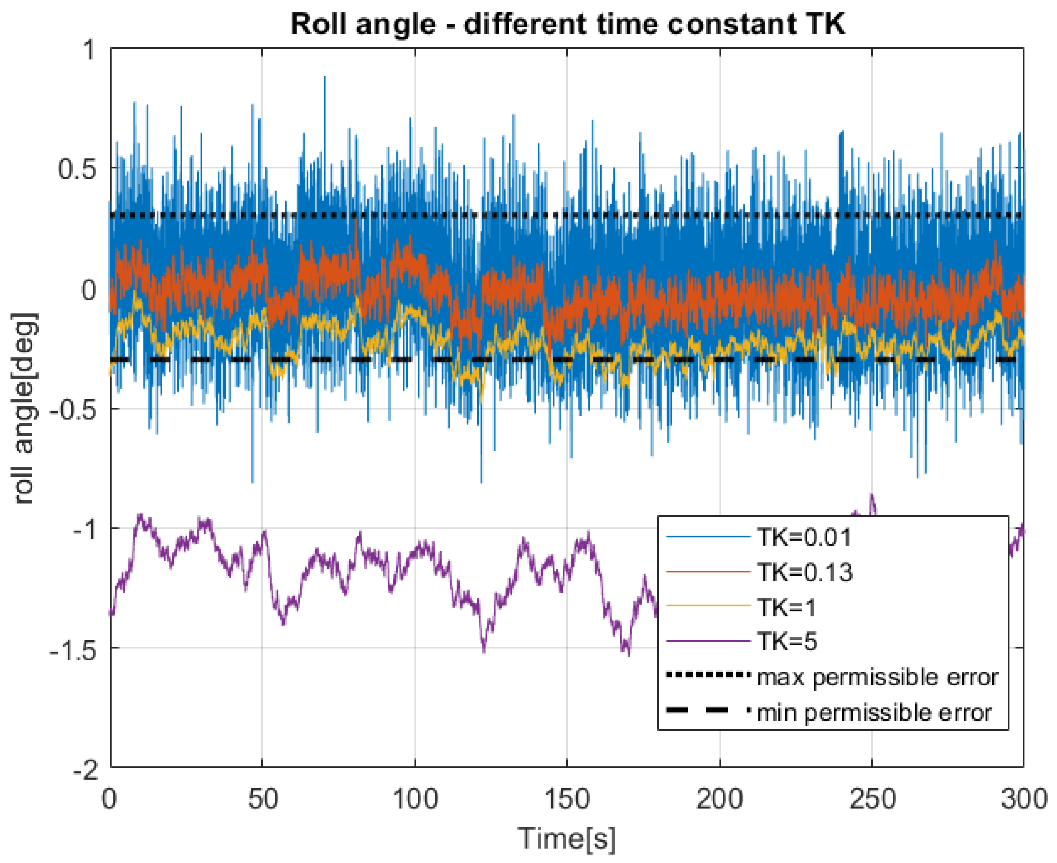
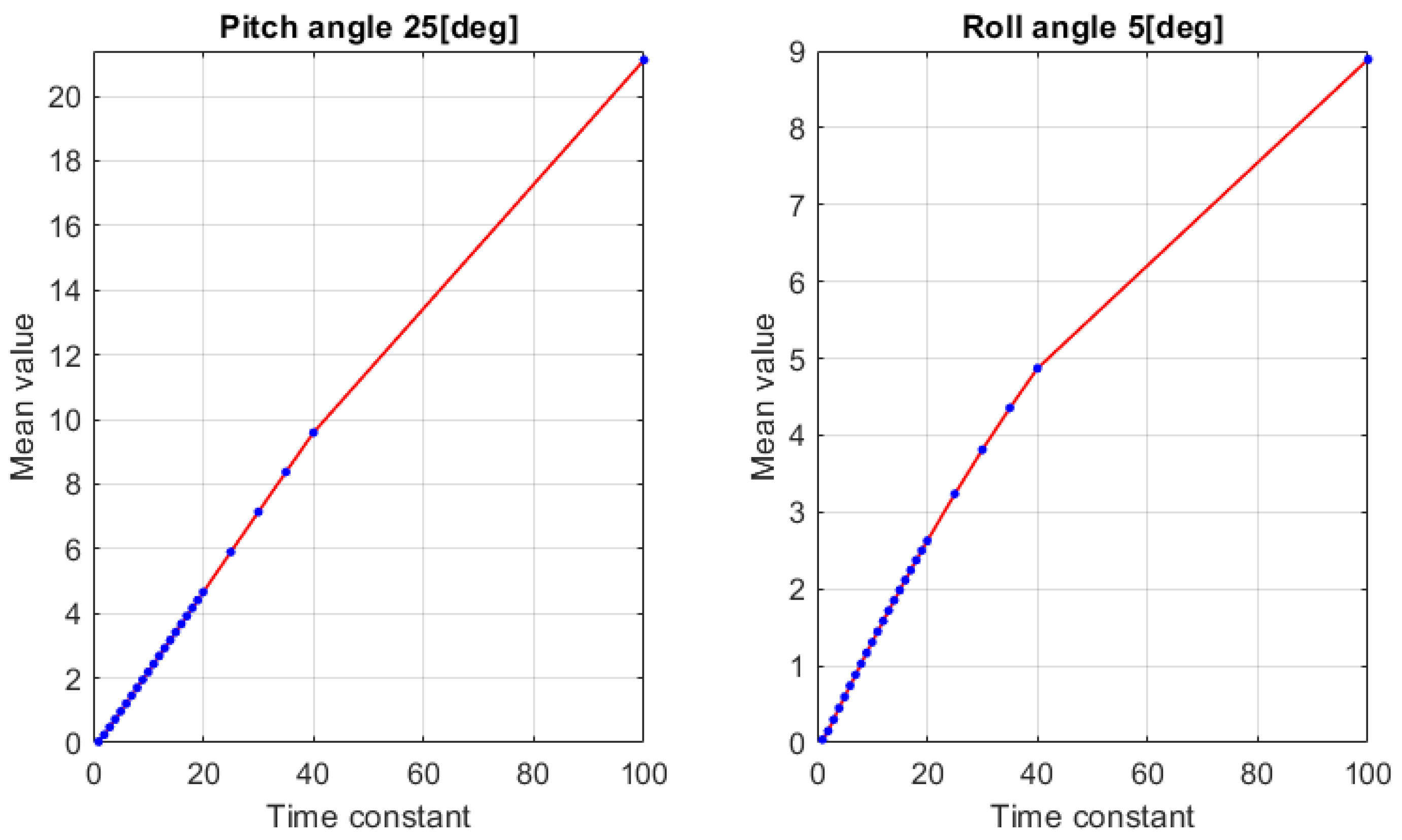
3.2. Optimization Methodology

In the first step, the output signal is transformed by centering it with respect to the true angle value. This transformation yields a time series of actual errors. The evaluation metric for the signal is the mean absolute error (MAE), expressed as a function of the complementary filter time constant (TC). This choice represents the most appropriate objective function for this optimization, as it operates in the same unit as the error, providing a direct and interpretable measure of the mean error. Alternative measures introduce functional distortions, affecting the physical meaning of the evaluated error.

The second step of the algorithm involves locating the minimum of the objective function through a “coarse” search. The range of time constant values, spanning from 1 to 100, is explored using a variable step size: between 1 and 20, the step size is fixed at 1, whereas beyond 20, it increases to 5 or more. This step size adjustment is informed by practical observations, leveraging the highly regular behavior of the MAE function with respect to the time constant. Such regularity facilitates efficient localization of the minimum.

The analysis was performed independently for roll and pitch angles, within the range of 0 to 30 degrees, with 5-degree increments. Below are example plots demonstrating the variation in MAE as a function of the time constant for roll at 5 degrees and pitch at 25 degrees.

Highly regular plots were obtained for all tested roll and pitch angles. Since these functions exhibit a minimum, it must reside within the interval $(0,1]$. This interval was explored with high precision, using a fixed step size of 0.01. Once again, highly consistent dependencies were observed for each angle. To illustrate this, we provide complementary plots for the angles described above.

To further quantify the observed regularities and precisely identify the optimal time constants, we summarize in the tables below the values at which the objective function—the mean absolute error (MAE)—reaches its minimum for the analyzed pitch and roll angles. These results provide a comprehensive summary of the behavior of the MAE function and demonstrate the high degree of regularity observed across the tested angles.

The analysis of the results reveals certain differences in the time constant values that minimize errors for various pitch and roll angles. For pitch angles, a universal time constant is determined as the average rounded to two decimal places. In this case, the optimal time constant is 0.12, for which the mean absolute error (MAE) remains below 0.05. For each attitude angle, the relations (Figure 7 and Figure 8) between the mean absolute error (MAE) and the time constant (TC) exhibit very regular and stable behavior. For different attitude angles, the location of the minimum remains stable and can be considered deterministic.

In the case of roll angles, minimizing errors for small angles is of greater importance. Hence, we applied a weighted average with the weights 0.6, 0.1, 0.1, 0.05, 0.05, 0.05, and 0.05, corresponding to the time constants for angles of 0, 10, 15, 20, 25, and 30 degrees, respectively. Using this approach, the optimal time constant is 0.15, with the MAE not exceeding 0.07.

Even without a deeper analysis of the data, the presented plots clearly demonstrate that improperly selected time constants can lead to errors several dozen times greater. This procedure is therefore critical to ensuring the precise operation of the system.

The next stage of the algorithm involves the detection of systematic errors, or, more specifically, trends in the output signal. Given the iterative and cumulative nature of the system’s operation, it is hypothesized that the trend should exhibit a linear character. To identify such errors, we employed a linear model for trend analysis.

Let the dependent variable y represent the centered signal, which corresponds to the error as a function of time. The systematic component of the error is modeled using a linear trend, while the residual term $ϵ$ captures the “pure error”. Mathematically, the model can be expressed as

$$y\left(t\right)={\beta }_0+{\beta }_{1}t+ϵ,$$

(15)

where ${\beta }_0$ represents the intercept, ${\beta }_1$ is the slope of the trend, and $ϵ$ is the residual error. This formulation allows for the separation of systematic biases (${\beta }_0+{\beta }_{1}t$) from the stochastic components ($ϵ$) in the centered signal. For each observed pitch and roll angle, the output signal exhibits distinct characteristics (see

Table 1. Optimal TC and corresponding minimum MAE for observed pitch and roll angles.

Pitch Angle	TC	Minimum MAE	Roll Angle	TC	Minimum MAE
0	0.11	0.049626	0	0.13	0.069190
5	0.12	0.048810	5	0.19	0.051458
10	0.13	0.047545	10	0.17	0.052601
15	0.13	0.048458	15	0.16	0.057899
20	0.12	0.046747	20	0.17	0.056838
25	0.12	0.046995	25	0.19	0.052498
30	0.12	0.049422	30	0.19	0.050939

) caused by slightly different systematic errors. Therefore, it is necessary to approximate the systematic errors in the signal for each observed angle individually and subsequently select the optimal model for the systematic error. The null hypothesis for the intercept term is formulated as $(H_0:\beta =0)$. If this hypothesis is rejected, it indicates the presence of a systematic (constant) error in the model. Similarly, the null hypothesis for the coefficient of the variable t is $(H_0:{\beta }_1=0)$, suggesting that t has a statistically significant effect on the dependent variable. If this hypothesis is rejected, it suggests that t has a statistically significant effect on the dependent variable.

In the case of roll angles, all null hypotheses were rejected, indicating the presence of both constant and time-dependent trends in the systematic errors. For pitch angles, however, the analysis revealed two specific cases of 10 and 25 degrees, where the coefficient of the time variable was not statistically significant, suggesting that only a constant trend is present for these angles. In the following, we provide the coefficients for each angle analyzed (

Table 2. LM coefficients for observed pitch and roll angles.

Pitch Angle	0_LM	5_LM	10_LM	15_LM	20_LM	25_LM	30_LM
(Intercept)	0.043588	0.026875	0.025521	0.035361	0.037425	0.034270	0.026435
t	−0.000055	0.000033	0.000000	−0.000044	−0.000052	0.000000	0.000038
Roll Angle	0_LM	5_LM	10_LM	15_LM	20_LM	25_LM	30_LM
(Intercept)	0.010557	−0.014750	−0.026526	−0.030684	−0.020162	−0.018307	−0.023530
t	−0.000305	−0.000055	−0.000004	0.000020	−0.000042	−0.000039	−0.000010

).

The next step involves removing systematic errors from the signal. Similarly to the process of selecting the optimal time constant, we chose to average the trend function. For roll angles, we applied a weighted average, while for pitch angles, we used a simple mean.

$$\mathrm{The}\mathrm{systematic}\mathrm{error}\mathrm{of}\mathrm{the}\mathrm{roll}\mathrm{angle}=-0.00242755-0.00019245t,$$

(16)

and

$$\mathrm{The}\mathrm{systematic}\mathrm{error}\mathrm{of}\mathrm{the}\mathrm{pitch}\mathrm{angle}=0.03278214-1.3e-0.0000114t,$$

(17)

where t is time. In the next subsection, we will analyze the optimized signal after the removal of systematic errors.

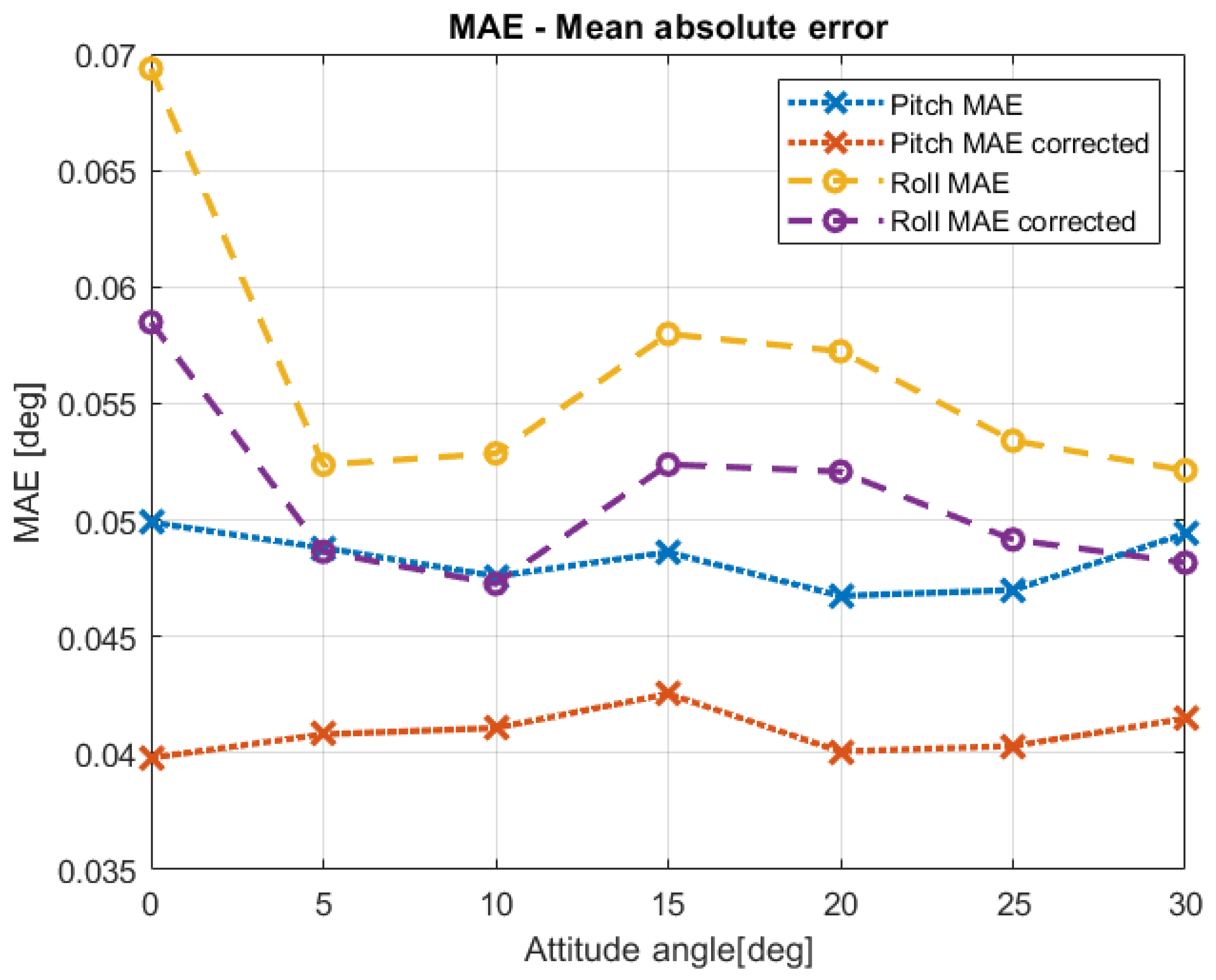
3.3. Performance Evaluation of the Optimized Signal

First, we compare how the algorithm reduced the mean absolute error (MAE) for individual angle values. This evaluation highlights the effectiveness of the algorithm in minimizing systematic errors across the tested pitch and roll angles. The summarized results are visualized in the Figure 9, illustrating the reduction in MAE achieved for each angle. A detailed analysis follows to interpret these findings.

A significant reduction in the mean absolute error (MAE) is evident, with decreases ranging from at least $15\%$ to nearly $25\%$. The maximum permissible absolute error was set at $0.5\%$ of the roll and pitch angle range. In this study, we adopted a range of $\pm 30$°, which translates to a maximum permissible error of $\pm 0.30$°.

Analyzing the signal, we observe that the maximum positive error for the pitch angle is 0.2035°, while for the roll angle, it is 0.2898°. These values remain well within the defined error tolerance. Similarly, the maximum absolute negative errors for pitch and roll angles are 0.2142 and 0.2759, respectively. This indicates that both the maximum and minimum error values comply with the permissible error criterion, providing an additional safety margin. Thus, the established goal was achieved successfully.

The graphical representation below (Figure 10) provides a clear visualization of these maximum and minimum error values, highlighting their compliance with the permissible error tolerance.

In addition to these observations, the mean squared error (MSE) values, which range from 0.002 to 0.005 across the angles analyzed, offer further insight into the filter’s performance. Given that the permissible absolute error is 0.3, these small MSE values indicate that the errors are tightly clustered around zero. This demonstrates the high precision achieved through the optimization of the complementary filter parameters.

The detailed MSE values for the observed pitch and roll angles are presented in

Table 3. MSE and RMSE for observed pitch and roll angles.

Roll Angle	MSE	RMSE	Pitch Angle	MSE	RMSE
0	0.005352	0.073161	0	0.002493	0.049934
5	0.003722	0.061010	5	0.002609	0.051075
10	0.003526	0.059377	10	0.002682	0.051790
15	0.004319	0.065719	15	0.002828	0.053177
20	0.004270	0.065346	20	0.002550	0.050495
25	0.003805	0.061685	25	0.002570	0.050691
30	0.003597	0.059972	30	0.002725	0.052202

, further supporting the robustness of the applied methodology.

We further propose a set of metrics to evaluate signal behavior in scenarios where either it exceeds the maximum permissible error threshold or, due to specific requirements, this threshold is deliberately narrowed to assess the extent of its reduction. The principal metric quantifies the occurrences of signal excursions beyond the specified limits, comprising the number of crossings above the upper limit, below the lower limit, and the total number of excursions outside the permissible range, calculated as the sum of the preceding two quantities. These metrics enable the estimation of the probability that the signal exceeds the prescribed boundary conditions.

We conducted observations with the boundary set at four times the mean absolute error, i.e., $\pm 0.168$ for the pitch angle and $\pm 0.232$ for the roll angle. This boundary is significantly tighter than the standard permissible limits defined earlier. Below, we present a table summarizing the predicted probabilities (

Table 4. Crossing probability for pitch and roll angles.

P_Ang	Pr_Up	Pr_Down	Pr	R_Ang	Pr_Up	Pr_Down	Pr
0	0.000467	0.001133	0.001600	0	0.000467	0.001200	0.001667
5	0.000867	0.001200	0.002067	5	0.002000	0.000133	0.002133
10	0.000933	0.001733	0.002666	10	0.002067	0.000067	0.002133
15	0.000400	0.000533	0.000933	15	0.000667	0.000067	0.000733
20	0.001200	0.000933	0.002133	20	0.002133	0.000133	0.002267
25	0.001533	0.000933	0.002467	25	0.001200	0.000200	0.001400
30	0.000867	0.001000	0.001867	30	0.000867	0.000067	0.000933

).

The up-crossing and down-crossing probabilities, representing the likelihood of exceeding the upper and lower boundaries, are both approximately ${10}^{-4}$. The overall probability of exceeding the boundary, combining both up-crossing and down-crossing events, is in the order of ${10}^{-3}$, indicating that such occurrences are extremely rare. This metric provides information about individual excursions, which theoretically last for a duration of $0.02$ s.

To provide a more comprehensive picture, it is necessary to analyze the number and duration of continuous sequences (time intervals) during which the signal exceeds the defined range. This allows for the estimation of the probability that the signal remains above or below the threshold for a specified duration, which is a multiple of $0.02$ s. Recall that $0.02$ s corresponds to the sampling period, and this multiple refers to the number of consecutive samples within a single uninterrupted sequence that stay above or below the threshold. For such an analysis, it is useful to include the ratio of the time spent outside the threshold to the subsequent time the signal remains within the range. This will allow us to observe whether the signal briefly returns to the range only to exit it again, and how frequently such situations occur. These two metrics enable a significantly more detailed understanding of the signal’s behavior. In our experiment, after narrowing the range, we observed only sporadic continuous sequences of the signal exceeding the threshold.

4. Conclusions, Discussion, and Future Work

In this work, the calibration of the time constant of the complementary filter for the AHRS system was performed. The presented methodology allowed for the selection of the optimal time constant value, which directly impacted measurement accuracy. The main objective of the study was to determine the time constant at which the error is minimized. After optimal tuning, the complementary filter transmitted the signal with an absolute error smaller than the maximum permissible absolute error. Both objectives were achieved, and most importantly, the signal remained entirely within the required error range with a significant margin. The complementary filter, despite its simplicity, provides high accuracy when the time constant is properly selected, which is sufficient for flight control tasks. Therefore, it can be successfully used in low-cost AHRS systems and implemented in relatively simple and inexpensive microprocessor-based systems. The methodology presented in this work is a tool that can be applied for scaling and evaluating AHRS systems in static conditions, without complicating the scaling process. For the scaling process, it is necessary to collect attitude in static conditions at seven different attitude angles, which does not require specialized test equipment. It was proposed to analyze attitude angles of 0, 5, 10, 15, 20, 25, and 30 degrees. In practice, it may even be possible to reduce the number of analyzed attitude angles. Limiting the data allows for more efficient tuning, which reduces the duration of system calibration. As a result of this research, we will develop software with the ability to analyze even larger amounts of data. As the first step of the algorithm, it will identify a unit-length interval containing the minima and recommend conducting measurements for such time constants with a step of 0.01. Finally, it will provide the optimization result. Each calculation step should take no more than one minute.

The results of this study show that the proposed algorithm to select the time constant provided the desired accuracy of measurements with a significant margin, and the maximum error did not exceed the range of the maximum tolerable error. The errors were concentrated around zero, and the maximum values were small. To assess the properties of the measured signal more precisely, an additional measure was proposed. A methodology to narrow the error values was demonstrated, which facilitates the evaluation of system properties. The probability of exceeding such a proposed range could serve as a new measure of the quality of measurement systems that meet predefined total error conditions. This can be useful, for instance, when comparing two different measurement systems that meet the specified requirements.

Our future research will focus on using the stationary test results as a baseline for identifying and compensating for errors in angle measurements during flight. The presented methodology does not account for errors caused by system vibrations. These baseline errors will act as a “reference signature”, enabling the development of correction mechanisms to mitigate the effects of vibration-induced disturbances. Such mechanisms are essential to ensure precise angle measurements, even in challenging operational environments. Measurement errors influence aircraft control quality. Their impact depends on the structure of the control mode, the control algorithm, the signals used for control, and the controlled aircraft properties. Details will be presented in further research.

Ultimately, the insights gained from stationary testing will support the training of predictive models capable of estimating errors in low-cost AHRS, paving the way for improved reliability in practical applications.

References

1. Kowalik, R.; Łuksiak, T.; Novak, A. A Mathematical Model for Controlling a Quadrotor UAV. Trans. Aerosp. Res. 2021, 3, 58–70. [Google Scholar] [CrossRef]
2. Steffensen, R.; Ginnell, K.; Holzapfel, F. Practical System Identification and Incremental Control Design for a Subscale Fixed-Wing Aircraft. Actuators 2024, 13, 130. [Google Scholar] [CrossRef]
3. Pecho, P.; Velky, P.; Kapustik, S.; Novak, A. Use of Computer Simulation to Optimize UAV Swarm Flying. In Proceedings of the 2022 New Trends in Aviation Development (NTAD), Novy Smokovec, Slovakia, 24–25 November 2022. [Google Scholar] [CrossRef]
4. Kusmirek, S.; Socha, V.; Urban, D.; Hanakova, L.; Kripsky, F.; Walton, R.; Pecho, P. Design of Pitot-Static Tube Shapes and Their Influence on Airspeed Measurement Accuracy. J. Aerosp. Eng. 2024, 37, 04024045. [Google Scholar] [CrossRef]
5. Qu, G.; Zhou, Z.; Li, J.; Shao, Z.; Dong, Y.; Guo, A. UAV Attitude Angle Measurement Method Based on Magnetometer-Satellite Positioning System. Appl. Sci. 2022, 12, 5947. [Google Scholar] [CrossRef]
6. Sedlackova, A.N.; Kurdel, P.; Mrekaj, B. Synthesis criterion of ergatic base complex with focus on its reliability. In Proceedings of the 2017 IEEE 14th International Scientific Conference on Informatics, INFORMATICS 2017, Poprad, Slovakia, 14–16 November 2017; pp. 318–321. [Google Scholar] [CrossRef]
7. Kopecki, G.; Dołęga, B.; Rzucidło, P. Fault Detection and Identification in the Doubled Attitude and Heading Reference System (AHRS). Sensors 2025, 25, 1603. [Google Scholar] [CrossRef]
8. Islam, M.S.; Shajid-Ul-Mahmud, M.; Islam, T.; Amin, M.S.; Hossam-E-Haider, M. A low cost MEMS and complementary filter based attitude heading reference system (AHRS) for low speed aircraft. In Proceedings of the 2016 3rd International Conference on Electrical Engineering and Information Communication Technology (ICEEICT), Dhaka, Bangladesh, 22–24 September 2016; pp. 1–5. [Google Scholar] [CrossRef]
9. Madgwick, S.O.H.; Harrison, A.J.L.; Vaidyanathan, R. Estimation of IMU and MARG orientation using a gradient descent algorithm. In Proceedings of the 2011 IEEE International Conference on Rehabilitation Robotics, Zurich, Switzerland, 29 June–1 July 2011; pp. 1–7. [Google Scholar] [CrossRef]
10. Zarchan, P.; Musoff, H. Fundamentalsof Kalman Filtering: A Practical Approach, 3rd ed.; American Institute of Aeronautics and Astronautics, Inc.: Reston, VA, USA, 2009. [Google Scholar]
11. Collinson, R.P.G. Introduction to Avionics; Chapman & Hall: London, UK, 1996. [Google Scholar]
12. Grygiel, R.T.; Bieda, R. Angles from gyroscope to complementary filter in IMU. Przegląd Elektrotechniczny 2014, 90, 217–224. [Google Scholar] [CrossRef]
13. Narkhede, P.; Poddar, S.; Walambe, R.; Ghinea, G.; Kotecha, K. Cascaded Complementary Filter Architecture for Sensor Fusion in Attitude Estimation. Sensors 2021, 21, 1937. [Google Scholar] [CrossRef] [PubMed]
14. Kopecki, G.; Rogalski, T. Aircraft Attitude Calculation with the Use of Aerodynamic Flight Data as Correction Signals. Aerosp. Sci. Technol. 2013, 32, 267–273. [Google Scholar] [CrossRef]
15. Li, X.; Xu, Q.; Shi, Q.; Tang, Y. Complementary Filter for Attitude Estimation Based on MARG and Optical Flow Sensors. J. Phys. Conf. Ser. 2021, 2010, 012160. [Google Scholar]
16. Pitieeraphab, Y.; Jusing, T.; Chotikunnan, P.; Thongpance, N.; Lekdee, W.; Teersoradech, A. The Effect of Average Filter for Complemetary Filter And Kalman Filter Based on Measurement Angle. In Proceedings of the 2016 Biomedical Engineering International Conference, Laung Prabang, Laos, 7–9 December 2016; BMEiCON-2-16. [Google Scholar]
17. Poulose, A.; Senouci, B.; Han, D.S. Performance Analysis of Sensor Fusion Techniques for Heading Estimation Using Smpartphone Sensors. IEEE Sens. J. 2019, 19, 12369–12380. [Google Scholar]
18. Wag, Y.; Li, N.; Chen, X.; Liu, M. Design and Implementation of an AHRS Based on MEMS Sensors and Complementary Filtering. Adv. Mech. Eng. 2014, 6, 214726. [Google Scholar] [CrossRef]
19. Ryzhkov, L. Complementary Filter Design for Attitude Determination. In Proceedings of the IEEE 5th International Conference on Methodz and Systems on Navigation and Motion Control (MSNMC), Kyiv, Ukraine, 16–18 October 2018. [Google Scholar]
20. Valenti, R.G.; Dryanovski, I.; Xiao, J. Keeping a Good Attitude: A Quaternion-Based Orientation Filter for IMUs and MARGs. Sensors 2015, 15, 19302–19330. [Google Scholar] [CrossRef] [PubMed]
21. Meyer, J.; Padayachee, K.; Broughton, B.A. A robust complementary filter approach for attitude estimation of unmanned aerial vehicles using AHRS. In Proceedings of the 2019 CEAS EuroGNC Conference, Milan, Italy, 3–5 April 2019; CEAS-GNC-2019-036. [Google Scholar]
22. Rzucidło, P.; Kopecki, G.; Szczerba, P.; Szwed, P. Analysis of Stochastic Properties of MEMS Accelerometers and Gyroscopes Used in the Miniature Flight Data Recorder. Appl. Sci. 2024, 14, 1121. [Google Scholar] [CrossRef]
23. Yoo, T.S.; Hong, S.K.; Yoon, H.M.; Park, S. Gain-scheduled complementary filter design for a MEMS based attitude and heading reference system. Sensors 2011, 11, 3816–3830. [Google Scholar] [CrossRef] [PubMed] [PubMed Central]
24. Thomas, D.; Mohit, V.; Christophe, C. Complementary Filters Shaping Using Hinf Synthesis. In Proceedings of the 2019 7th International Conference on Control, Mechatronics and Automation (ICCMA), Delft, The Netherlands, 6–8 November 2019; pp. 459–464. [Google Scholar] [CrossRef]
25. Duong, D.Q.; Sun, J.; Nguyen, T.P.; Luo, L. Attitude estimation by using MEMS IMU with Fuzzy Tuned Complementary Filter. In Proceedings of the 2016 IEEE International Conference on Electronic Information and Communication Technology (ICEICT), Harbin, China, 20–22 August 2016; pp. 372–378. [Google Scholar] [CrossRef]
26. Kopecki, G.; Tomczyk, A.; Rzucidło, P. Algorithms of Measurement System for a Micro UAV. Solid State Phenom. 2013, 198, 165–170. [Google Scholar] [CrossRef]
27. Kopecki, G.; Banicki, M. A proposal of AHRS yaw angle correction with the use of roll angle. Aircr. Eng. Aerosp. Technol. 2023, 95, 1435–1443. [Google Scholar] [CrossRef]
28. Dolega, B.; Kopecki, G.; Tomczyk, A. Possibilities of using software redundancy in low cost aeronautical control systems. In Proceedings of the 3rd IEEE International Workshop on Metrology for Aerospace (MetroAeroSpace) 2016, 2016 IEEE Metrology for Aerospace (Metroaerospace), Florence, Italy, 22–23 June 2016; pp. 33–37. [Google Scholar]
29. Rzucidlo, P.; Kopecki, G.H.; deGroot, K.; Kucaba-Pietal, A.; Smusz, R.; Szewczyk, M.; Szumski, M. Data acquisition system for PW-6U in flight boundary layer mapping. Aircr. Eng. Aerosp. Technol. 2016, 88, 572–579. [Google Scholar]
30. Kopecki, G.; Rzucidlo, P. Integration of optical measurement methods with flight parameter measurement systems. Meas. Sci. Technol. 2016, 27, 054003. [Google Scholar] [CrossRef]
31. Durham, W. Aircraft Flight Dynamics and Control; John Wiley & Sons, Ltd.: Hoboken, NJ, USA, 2013. [Google Scholar]
32. Gosiewski, Z.; Ortyl, A. Algorithms of an Inertial Gimbal-Free Orientation and Positioning System for an Object in Spatial Motion; Scientific Publishing House of the Institute of Aviation: Warsaw, Poland, 1999; ISBN/ISSN 83-910906-1-2. (In Polish) [Google Scholar]
33. Tomczyk, A. Testing of the attitude and heading reference system. Aircr. Eng. Aerosp. Technol. 2002, 74, 154–160. [Google Scholar] [CrossRef]
34. Gruszecki, J. (Ed.) Unmanned Aerial Vehicles: Control and Navigation Systems; Oficyna Wydawnicza Politechniki Rzeszowskiej: Rzeszów, Poland, 2002. (In Polish) [Google Scholar]
Figure 1. Attitude and heading reference system—general scheme.
Applsci 15 04114 g001
Figure 2. Measurement system with a complementary filter—a general scheme.
Applsci 15 04114 g002
Figure 3. Complementary filter for attitude estimation.
Applsci 15 04114 g003
Figure 4. Example of registered angular rates.
Applsci 15 04114 g004
Figure 5. Example of registered accelerations.
Applsci 15 04114 g005
Figure 6. Example of roll angle for different time constants TK.
Applsci 15 04114 g006
Figure 7. The dependence of MAE on TC for values in the range of 1 to 100.
Applsci 15 04114 g007
Figure 8. MAE variation as a function of TC in the range from 0.01 to 1.
Applsci 15 04114 g008
Figure 9. Reduction in mean absolute error (MAE) for observed angles.
Applsci 15 04114 g009
Figure 10. Maximal and minimal errors for pitch and roll angles.
Applsci 15 04114 g010