1. Introduction
As the backbone of the transportation system, railway transportation has the advantages of large capacity and high efficiency. With the development of railway construction, locomotive traction power is also increasing, and the locomotive traction power depends on the adhesion between the wheel and rail. When the rail surface condition deteriorates, with the increase in traction torque and the acceleration of creep velocity, the driving force between the wheel and rail is greater than the maximum adhesion force that the wheel and rail can provide; excess force causes the wheelset to rotate sharply, causing the adhesion to be destroyed and further reducing the available adhesion force, making the condition worse and resulting in slipping and sliding. Once the wheelset slips, the locomotive driving force will suddenly drop, or even disappear, which will lead to a decrease in velocity. In severe cases, it will even lead to rail scratches and wheelset set tread peeling. Locomotives experience similar effects in the case of braking: excess braking force will cause the wheelset velocity to be lower than the vehicle velocity, resulting in sliding. In severe cases, the wheelset will be locked, which causes serious damage to the wheelset and the track [
1]. It is of great significance to effectively predict slipping in order to enhance locomotive operation safety and reduce energy loss. During locomotive operation, the TCU produces large amounts of operation data, which provide a large number of samples for analysis by researchers, and the multiple wheel shaft slipping states in these data constitute the timing information that is mainly analyzed in this paper. The ability to predict the slipping states efficiently and accurately is the focus of this paper.
In recent years, there have been many studies on slipping detection and adhesion control. The hybrid adhesion control method is a widely used adhesion control method [
2,
3,
4]. This method first calculates slip velocity, acceleration, and acceleration differential, then compares them with predefined thresholds to determine whether the locomotive has slipped based on numerical values and conditions. However, this approach is susceptible to wheel–rail noise interference, relies on manually set parameters, and introduces human-induced errors, ultimately affecting detection accuracy.
With the advancement of machine learning and deep learning algorithms, some machine learning algorithms, such as neural networks, clustering, and other methods, have begun to be applied to state estimation. Reference [
5] proposes a method combining fuzzy neural networks and unscented Kalman filtering for train anti-slip control. UFK is suitable for the time domain filtering of recursive Gaussian linear systems, and performs well in the state estimation of dynamic linear systems subject to Gaussian distribution. However, in complex and changeable environments, UFK performs poorly and has poor robustness. Moreover, fuzzy neural networks have high computational complexity, difficult rule optimization, low interpretability, and limited generalization ability. Reference [
6] proposes a locomotive slipping detection method based on empirical wavelet transform (EWT), fuzzy entropy (FE), and SVM. The algorithm decomposes the speed data by EWT, extracts the feature information related to slipping by the fuzzy entropy algorithm, and then trains and optimizes SVM by particle swarm optimization algorithm. The method has a high accuracy and recall rate, but the calculation process is complex and the detection rate is low. It cannot predict the locomotive data online in real time. Reference [
7] proposes a method that combines wavelet analysis with an LSTM+MLP model to extract short-term and long-term features of the slip state for slip detection and recognition. However, the computational load of this model is relatively high, which may result in slower response times and delays in feedback on the detected slip state. Reference [
8] proposes a slipping detection method based on a deep denoising auto-encoder. This method combines a self-encoder with a classification neural network, uses an auto-encoder to extract features, and inputs them into the classification network for prediction. This method performs poorly in the case of small samples, which can only identify the current moment’s wheel slip state and cannot be used for prediction. In reference [
9], a slipping recognition method based on Recurrent Neural Networks (RNN) [
10] is proposed. The method sends the time series data into the RNN. According to the output of the previous time, the current time input can excavate the correlation characteristics in the time series, but the output speed is slow. It needs to calculate the weighted sum of the eigenvalues of the previous time, and it can only decode the prediction step by step, and cannot predict the long-sequence results.
In summary, regardless of the method used, leveraging data characteristics to detect the slipping state is key to this type of research. In deep learning, classical networks such as fully connected neural networks and convolutional neural networks have strong feature extraction capabilities. However, as data passes through each network layer, feature loss occurs, and the receptive field problem grows. This leads to the failure of the last layer to capture all the features of the original data, resulting in poorer training performance as the number of network layers increases [
11]. ResNet [
12], proposed in 2016, effectively solved the problem of feature loss through feature concatenation and fusion. However, as the network layers are stacked, the computational load increases, the number of training parameters grows, and memory usage rises significantly. RNN and Long–Short-Term Memory Network (LSTM) [
13] are widely used in natural language processing (NLP) because of their strong ability to process sequential text data [
14]. However, RNN and LSTM do not have the ability of parallel output, and instead decode according to previously acquired information; thus, with an increase in text information, the output efficiency will become slow.
Transformer [
15], introduced in 2017, brought about a significant shift in feature extraction networks. With its encoder–decoder structure, it allows parallel prediction output and leverages a multi-head attention mechanism to model correlations in time-series data. Unlike CNNs, Transformer can effectively extract features without relying on deep network stacking, ensuring consistent feature representation across layers. However, a major drawback is its uniform attention distribution across all time steps, which can hinder the capture of global dependencies and make it more vulnerable to local noise, especially in long-range sequences. This ultimately affects prediction accuracy [
16]. To address these issues, Informer [
17] was proposed in 2020, refining the attention mechanism to improve efficiency. By filtering out redundant attention information, it significantly reduces computational costs and memory usage. The introduction of the ProbSparse self-attention mechanism helps to maintain focus on the most relevant key information, enhancing the capture of long-range dependencies while minimizing unnecessary calculations [
18]. Moreover, Informer incorporates timestamp encoding to better preserve sequence structure, and adopts a one-step decoder, enabling all predictions to be generated efficiently through a fully connected output layer.
In train slip detection, the key is to identify critical information about the slip state within long-sequence data. Therefore, this paper integrates the advantages of Informer’s ProbSparse self-attention mechanism and one-step decoder, improving the output structure of Transformer’s decoder and transforming the prediction model into a classification model without adding an extra classification branch. The model first encodes locomotive operation data from the initial few seconds to extract features, which are then fed into Informer. The decoder directly outputs the prediction results for the following seconds.
This paper compares the novel model with previous slipping state detection models, showing that it has the following four main advantages:
- (1)
It can predict the slipping state of the locomotive wheel shaft with n time steps, and has a high accuracy and recall rate.
- (2)
It can simultaneously predict the locomotive multi-axle slipping state.
- (3)
The prediction speed is fast, and prediction can be performed online.
- (4)
It can take into account the impact of some theoretically inexplicable association parameters in running data.
2. Preliminary
In
Figure 1,
is the wheel rolling radius;
is the wheel rotation angular velocity;
is the train’s speed;
is the locomotive load, also known as the positive pressure exerted on the track by the wheelset; and
is the tangential traction force acting on the wheel–rail contact surface, but is also the adhesion force.
“Adhesion” refers to the phenomenon that the wheel rolling has no relative slipping, and the wheel–rail contact remains relatively static during the locomotive’s operation [
19]. In
Figure 1, when the train is running, the wheel rolls under the action of torque T, and the wheel–rail contact surface bears the positive pressure exerted by the wheel on the rail. Because the wheel and rail are elastic bodies, under the action of axle load, the wheel–rail contact surface produces elastic deformation, forming an elliptical contact area. The contact area is divided into a slipping zone and an adhesion zone. The relative velocity in the adhesion zone is zero, and the creep occurs in the slipping zone, which makes the actual running distance of the train less than the pure rolling distance. When the wheel rolls, tangential adhesion between the wheel and rail, namely, traction around the wheel, is generated, and is the only power causing the train to move forward. In order to measure the adhesion force between the wheel and rail under different creep rates, the adhesion coefficient
is defined as the ratio of the wheel-rail adhesion force to the vertical load on the wheel [
20].
The adhesion force makes the medium of the wheel–rail contact surface move relatively, and the train velocity is less than the circumferential velocity of the wheel rolling, which is called creep [
21]. With an increase in applied torque, the area of the slipping zone increases. When a certain threshold is reached, the slipping zone will cover the entire contact surface, creep will rapidly develop into macro-slipping, and the wheel will slip [
22].
In order to measure the slipping degree, the slipping velocity
and the slipping rate
are defined as follows:
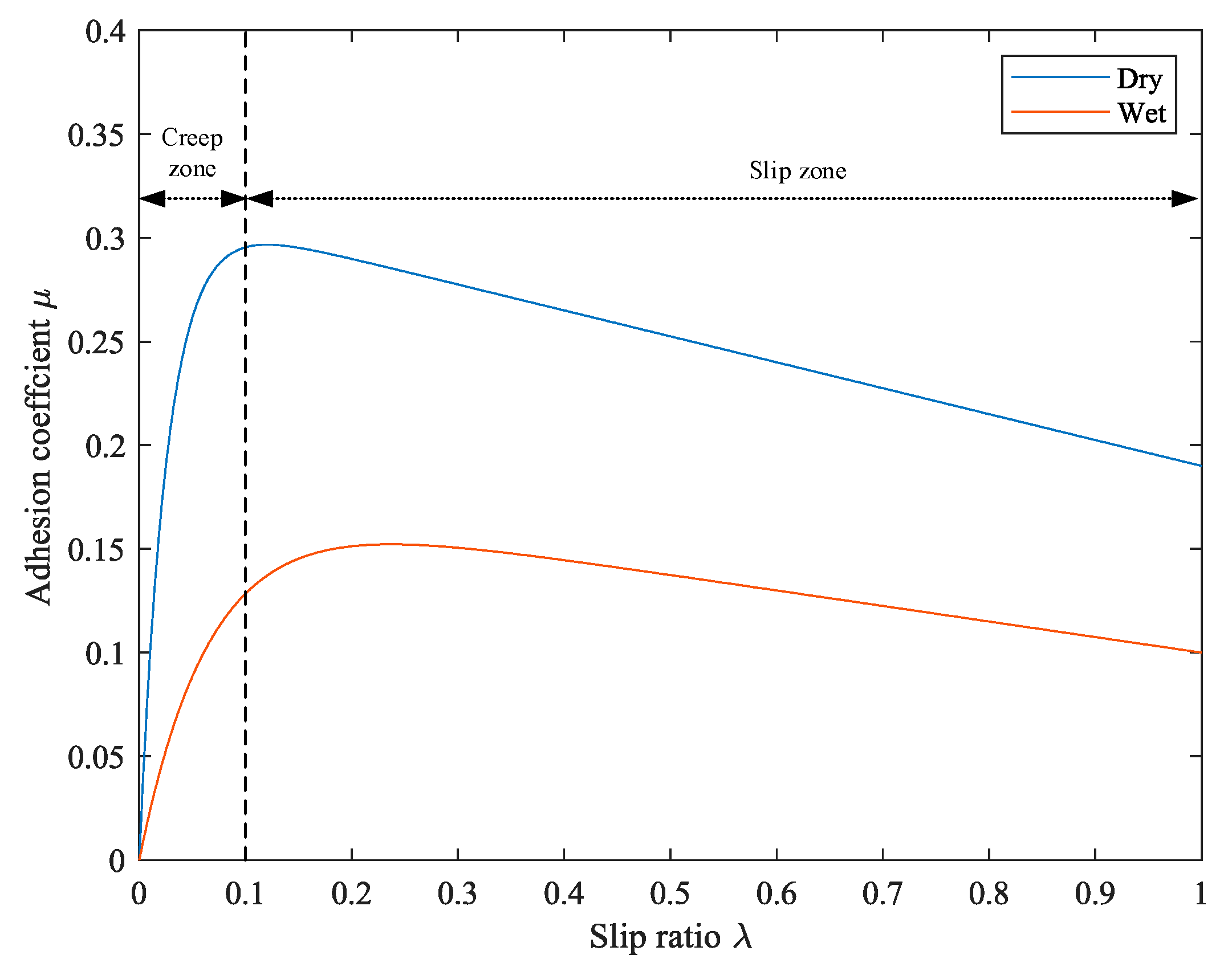
Adhesion is a very complex phenomenon that is affected by many conditions. Under different conditions, the adhesion characteristics are different.
Figure 2 shows the adhesion characteristic curve, showing the relationship between the slipping rate and adhesion coefficient under different rail surface conditions. At the point where the adhesion coefficient is the largest, the adhesion limit is reached. The adhesion limit divides the curve into two regions. The left side is the creep zone, and the right side is the slipping zone. In the creep zone, the wheel–rail contact characteristics are normal. If the creep rate exceeds the adhesion limit and enters the slipping zone, the wheel becomes prone to slipping.
3. Methodology
The creep classification prediction method based on Informer is a method to obtain a multi-axle two-classification prediction model by training on locomotive operation data.
This paper combines the advantages of Transformer and Informer to improve the output structure of the network, as shown in
Figure 3. Using the same encoder–decoder structure as Transformer, the feature matrix containing position information is obtained by value coding and position coding. Traditional full self-attention requires computing the attention weights between each
and all
, resulting in a computational complexity of
. When the sequence length is large, both the computational cost and memory consumption increase significantly. In contrast, ProbSparse self-attention leverages the long-tail distribution of attention weights by selecting only the top
n key positions with the most significant weight differences for detailed computation, while averaging the remaining parts. This approach significantly reduces computational complexity and memory usage, while ensuring that the most critical information receives sufficient attention, thereby improving overall computational efficiency. Therefore, ProbSparse is employed in this paper to extract relevant features.
Through the ProbSparse self-attention mechanism, the feature matrix obtains the attention relations of different feature vectors at different positions, and is parallelly calculated by the multi-head method. After completing the self-attention mechanism, in order to reduce the number of network parameters, the distillation pool operation is carried out, and the multi-head ProbSparse self-attention mechanism is carried out again. The input to the decoder is the splicing of the predicted results at some moments before the predicted moment and the filling value of the predicted length. In order to prevent autoregression, the joint attention mechanism is carried out with encoder’s temporal feature matrix after mask self-attention, and the slipping parameter information at different times is associated with the slipping state. Finally, the future time is predicted directly by full connection and the Sigmoid activation function.
3.1. Datasets
For the choice of model input, we consider multiple parameters, including velocity, wheel velocity, and shaft traction. Firstly, the number of selected parameters is defined as , the input length of the encoder in the model is , and the predicted output length of the decoder is . Considering the small proportion of the total amount of data when slipping occurs, in order to prevent overfitting of the normal state caused by sample imbalance, the datasets are filtered. The time series of several seconds before and after the slipping of four shafts is selected as data. The sequence is , and the input of the model is .
3.2. Embedding
- Step 1.
Value embedding
Firstly, the input
is extracted by a one-dimensional convolution to obtain the feature matrix
, where
is the input dimension of the model.
- Step 2.
Position Embedding
In order not to lose the timing information of each row vector of time series
, the position encoding of each row vector of time series
is needed. There are many ways to perform position coding; this paper uses relative position embedding based on trigonometric functions [
23].
- Step 3.
Embedding fusion
Finally, the input
of the attention network is obtained by adding a feature matrix
and position coding
. After only one convolution,
retains almost all the features of the original data, and contains temporal information between feature vectors in the original data.
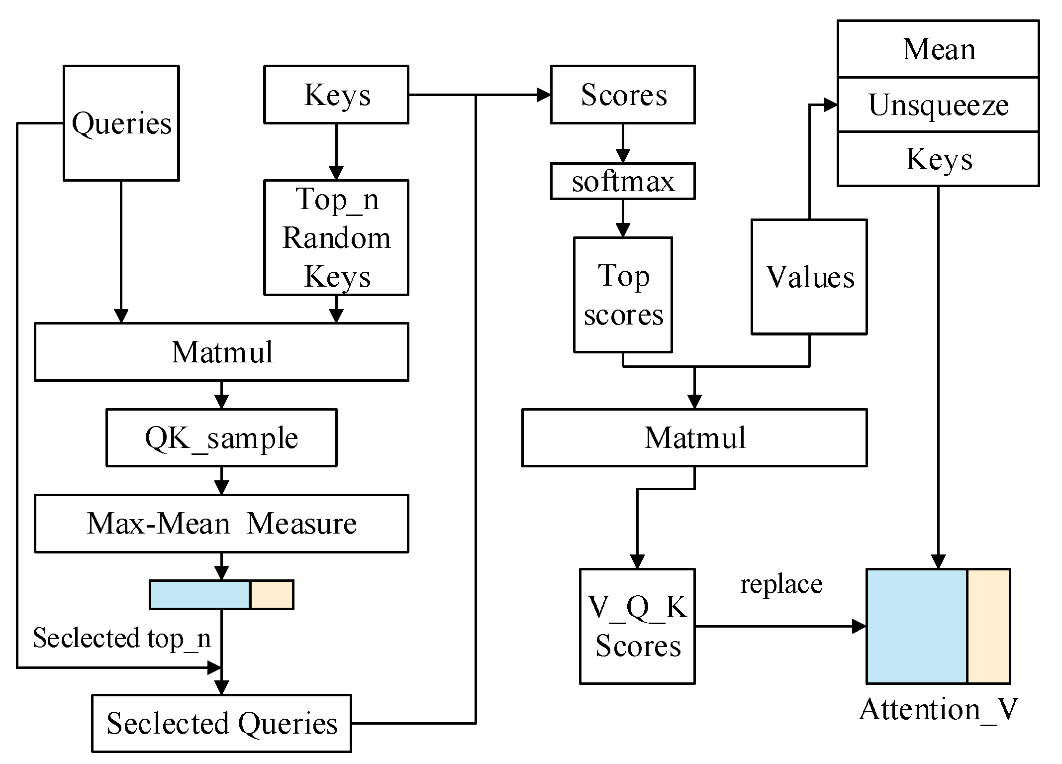
3.3. Multi-Head ProbSparse Self-Attention
The self-attention mechanism first divides
into multiple heads for parallel computing, and each head obtains three matrices,
,
, and
, through three full connection layers
. The Probsparse self-attention algorithm is shown in
Figure 4.
is the weight matrix,
is the bias,
is the dimension of each head, and
is the activation function, such as RELU.
and
obey the long-tailed distribution after passing the dot product, and only a small number of them generate the main attention, while the majority produce negligible attention values, resulting in computational redundancy. In order to reduce the amount of computation, the top n keys are randomly selected to obtain
, and then Max-Means Measurement is carried out with
to obtain the distribution difference between
and
, with the formula
.
is the length of
, and
is the same as
in the self-attention mechanism.
Figure 4.
ProbSparse self-attention algorithm graph.
Figure 4.
ProbSparse self-attention algorithm graph.
We expect that the distribution of attention varies greatly, with each unit attending to specific features instead of following a uniform pattern. The component exhibiting maximum distribution divergence is selected, and then the attention is calculated with
and
. Then, the remaining trivial attention part is averaged to obtain
.
3.4. Distilling
If the multi-layer self-attention mechanism is needed, the distillation pooling operation is used between each layer to reduce the number of parameters to be calculated and accelerate the forward propagation speed of the network [
24]:
where
is layer
after convolution and reshape operations.
is a down-sampling pooling operation with a step size of 2. At the same time, feature fusion is introduced before distillation, and the input of the upper layer and the output of the next layer are added to ensure that important features will not be lost when the network is deepened.
3.5. Decoder
This paper improves the classification prediction task by modifying the input to the Decoder. The input of the decoder is the splicing of the prediction results at some moments before the prediction time and the filling value with the predicted length . This allows the previously known slipping state to assist in the sequence prediction. The full zero filling is used in the original Informer. In the slipping state detection, when the predicted value of classification is 0 or 1, using full zero filling and full 1 filling will interfere with the prediction results. We use the Sigmoid function for the output of the model, and set the adjustable threshold so as to calculate the index. Here, we use the same value as the threshold to fill, such as 0.5, which eliminates the interference caused by full zero filling.
In the decoder’s self-attention layer, since we do not want future results to affect previous results, the masked self-attention mechanism is used in order to prevent self-regression. In the attention layer of the decoder, the attention relationship between the self-attention layer and the encoder’s output is computed, associating the parameter features influencing slipping with the slipping state. When analyzing this attention relationship, significant differences in distribution are observed, with fewer parameters corresponding to the slipping state. Here, ProbSparse attention is not applied; instead, full attention is used. The full attention mechanism follows the same formulation as Equation (13).
3.6. Forward Propagation and Prediction
After encoder–decoder is completed, the output is mapped to
with the same size as the slipping state through a full connection layer. Since the slipping state is directly selected as the input of the decoder, we do not need to add new classification branches in the output, but use the Sigmoid activation function to map the output to 0 and 1, and set the threshold for classification prediction.
When the predictor detects the slipping state, it will send a slipping signal to the controller, which performs adjustments by reducing the traction or braking force. When the slipping signal disappears, the controller adjusts the traction or braking force to normal.
3.7. Back-Propagation Training
The cross-entropy loss function [
25] is widely used in classification tasks. This paper uses this function as the loss estimation of the model, as shown in Formula (18):
SGD (Stochastic Gradient Descent) [
26] is widely used in various neural network learning tasks. The gradient term of this method does not add any momentum coefficient, and it is easy to fall into the local optimum, as shown in Formula (19).
where
is the weight parameter matrix at time t,
is the learning rate, and
is the gradient of the loss function to the weight. Obviously, the convergence speed and the final convergence effect of Adam (Adaptive Momentum Estimation) [
27] are better than other optimizers, as shown in
Figure 5. Adam adds both first-order momentum and second-order momentum to SGD. First, the first-order momentum
is calculated according to Formula (20):
The calculation of second-order momentum is the same as that of RMSProp [
28] and Adagrad [
29], as shown in Formula (21). This article does not introduce many other optimizers.
where
and
are exponential decay rates estimated twice. In order to prevent the gradient weight from being small at the beginning of training, two momentums are added to the correction factors
and
of the exponential weighted average, respectively, so that the sum of the weights of each time step in the training process is 1. The formula is derived as follows (
initialized to 0):
The relationship between the first-order momentum
and the gradient
is derived by the above formula:
The weight correction factor is deduced as Formula (25):
The calculation process of
is the same as that of
, so it is not repeated. By dividing the two momentums
and
by the corresponding correction factor, the corrected momentum is obtained:
Finally, the parameters of the Adam optimization algorithm are updated with Formula (28), where
is a minimum number, preventing the denominator from being 0.
4. Experiment
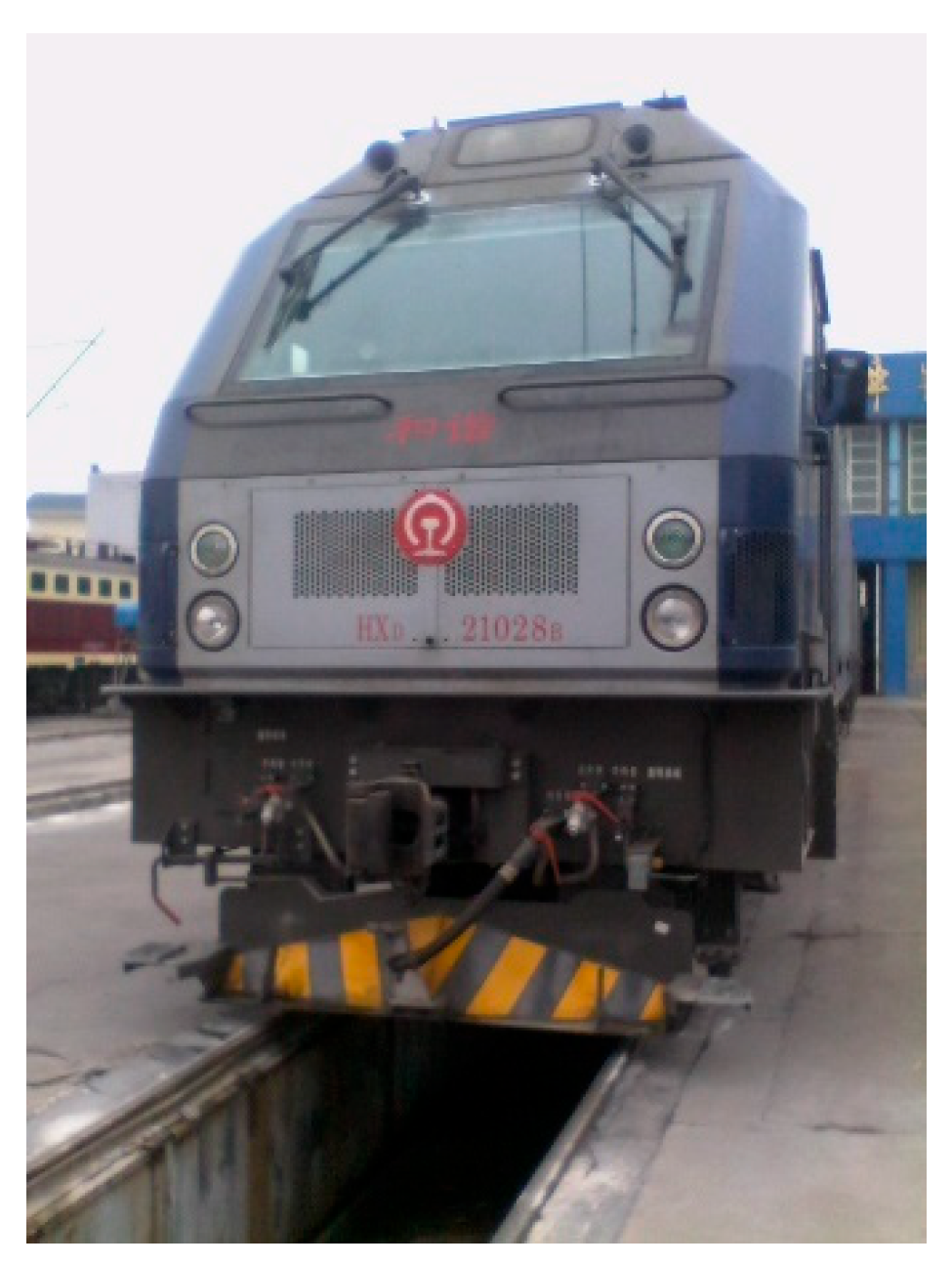
In order to prove the feasibility and effectiveness of the slipping classification prediction method based on Informer, a large number of experimental analyses of locomotive operation data were carried out. The HXD2 locomotive (
Figure 6) was used as the test locomotive. Its parameters are shown in
Table 1. The test line section was Xinfengzhen Station–Ankang East Station, within the jurisdiction of Xi’an Railway Administration. The gradient of the selected experimental line ranges from 6 to 12‰ and features continuous uphill and downhill sections; that is, we selected sections where the locomotive would be prone to slipping. The experimental data were actual operation data collected by the TCU. There is a data acquisition unit in the TCU of a locomotive, which can continuously collect data over several months, and these data can be applied for control, analysis, and maintenance.
The dataset comprised approximately 240,000 samples, with around 30,000 samples corresponding to slipping states. The data were partitioned into a training set and a testing set, constituting 80% and 20% of the total dataset, respectively. During this period, due to interference from the environment, it was expected that there would be missing or distorted sampling of the data, and the data used in the model training and testing were cleaned. Even if there are some disturbances, since the proposed model contains many dropout layers, it is robust and can effectively prevent the overfitting problem caused by these disturbances. Therefore, the impact of these disturbances on training and testing is small, and can be ignored.
4.1. Comparing Other Models
Since models such as RNN and LSTM cannot predict multiple time steps in the future at the same time, in the test set, the next second was predicted, and a comparative test was carried out, as illustrated in
Table 2. In the experiment, Informer and LSTM achieved high accuracy, but for slipping recognition, the recall rate is more important. Due to the multi-axle simultaneous prediction and the uneven proportion of slipping states, the recall rate is generally lower than the accuracy rate. In order to better measure the model in this task, this study calculated the F1 measure as the reference index.
4.2. Informer Model for Predicting Future Numbers of Seconds (Multi-Axle and Single-Axle)
The Informer classification prediction model proposed in this paper can simultaneously output the slipping state of four axes in the next few seconds. Limited by the uneven data of multi-axle synchronous prediction of slipping state, the recall rate fell in the experiment of predicting multiple time steps, but the model still had high accuracy, as shown in
Table 3.
For the single-axle prediction, the data distribution was more uniform than for the multi-axle prediction, which significantly improved the recall rate, as shown in
Table 4.
4.3. Model Failure and Edge Case Analysis
The improved Informer model achieved an overall accuracy of 94.75%, and outperformed RNN and LSTM in the experiments. However, certain issues remained, such as the potential failure of the model in some edge cases. As shown in
Table 3 and
Table 4, with an increase in the prediction horizon, the accuracy, recall, and F1 score exhibit a gradual decline. This may be due to error accumulation, which can degrade model performance in long-sequence forecasting and reduce prediction reliability, particularly in edge cases. Furthermore, in practical scenarios, the proportion of idle states is not balanced. Particularly in multi-axle predictions, idle states constitute a relatively small portion of the dataset, leading the model to focus more on non-idle states. As a result, it may fail to detect rare idle-state edge samples. Additionally, although dropout was applied to mitigate overfitting, the dataset consists entirely of real-world data from the Train Control Unit (TCU). Some data may contain significant errors due to sensor noise interference. Compared with the improved Informer model, traditional RNN and LSTM, with their internal state transmission and gating mechanisms, exhibit certain advantages in capturing long-term dependencies and smoothing out short-term anomalies. Future research will further explore hybrid models or design specialized robustness enhancement strategies for these edge cases to improve reliability while maintaining real-time prediction capabilities.
4.4. Analysis of Rotation Velocity and Axial Force Before and After Slipping
In the train operation data, the percentage of axial force can well represent the traction force of a single axle of the locomotive, and the calculation formula is as follows:
where
is the percentage of axial force and
is the uniaxial traction force. The percentage of single-axle axial force in a certain period is shown in
Figure 7. After the locomotive reaches the maximum torque (50 s), multiple slipping phenomena occur after 150 s, resulting in a significant decrease in axial force. The improved Informer proposed in this paper can well extract relevant characteristics and classify and predict the slipping state. ROC is often used to evaluate the classifier, which can compare the detection ability of different methods. The dashed diagonal line in the ROC plot represents the performance of a random classifier. The closer the ROC curve is to the top-left corner and the farther above the diagonal line it lies, the better the classifier performs. The closer to the upper left corner of the curve, the better the method. The area under the curve is called the AUC (Area Under Curve), and the size of the AUC can reflect the detection capability more clearly. As can be seen from
Figure 7, the ACU with axle traction is 0.992, and the AUC without axle traction is 0.973, which indicates that the parameter works.
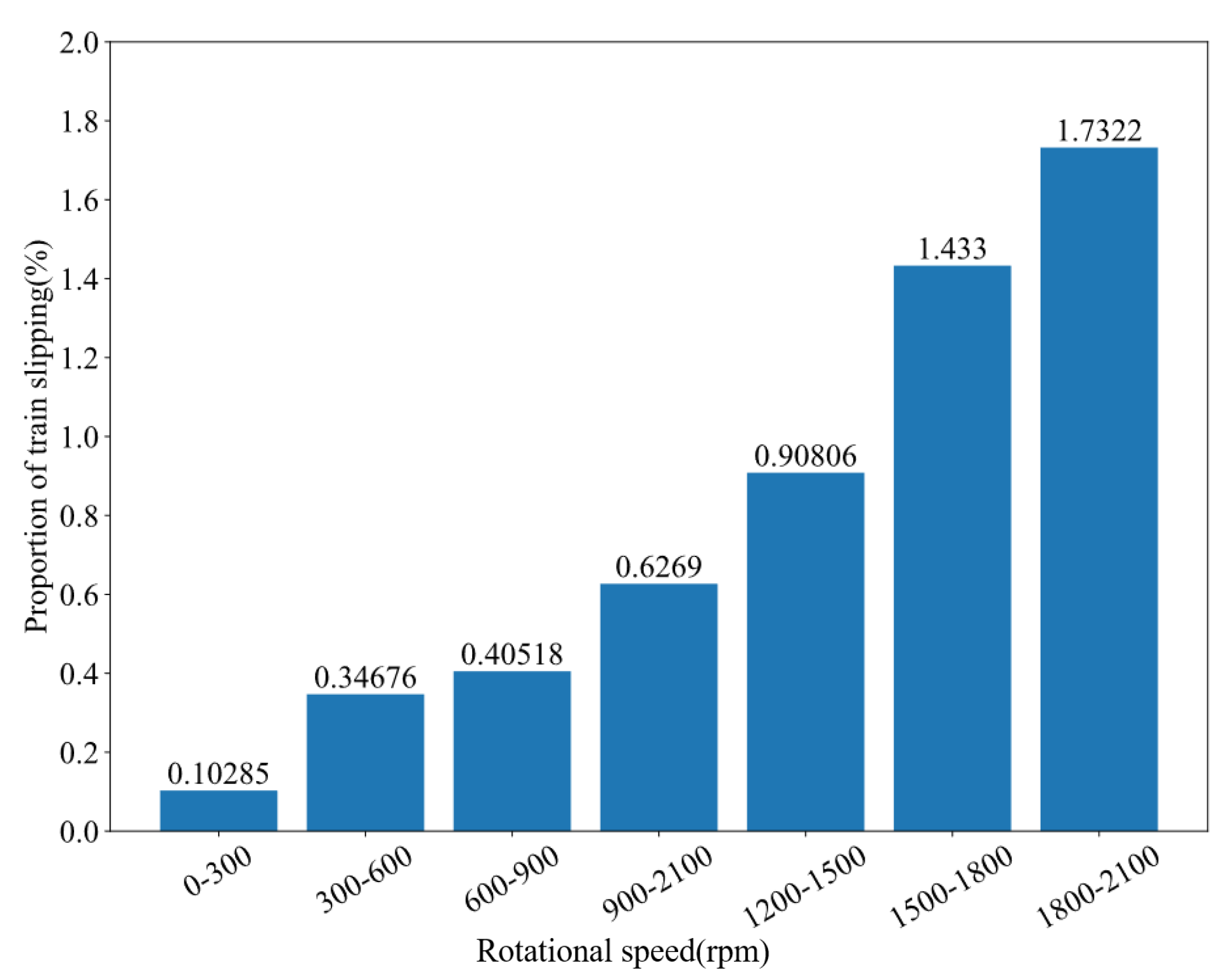
In order to make the slipping more intuitive, we counted the proportion of slipping at each stage of velocity from 0 to 2100 rpm. The percentage of slipping in each speed range is shown in
Figure 8. From the data analysis, it can be seen that the slipping rate is as high as 1.73% at 1800 to 2100 rpm, which shows that slipping phenomena are more likely to occur at high speeds. In the model proposed in this paper, the weights of neural networks can be affected by these auxiliary parameters, so as to improve the performance.
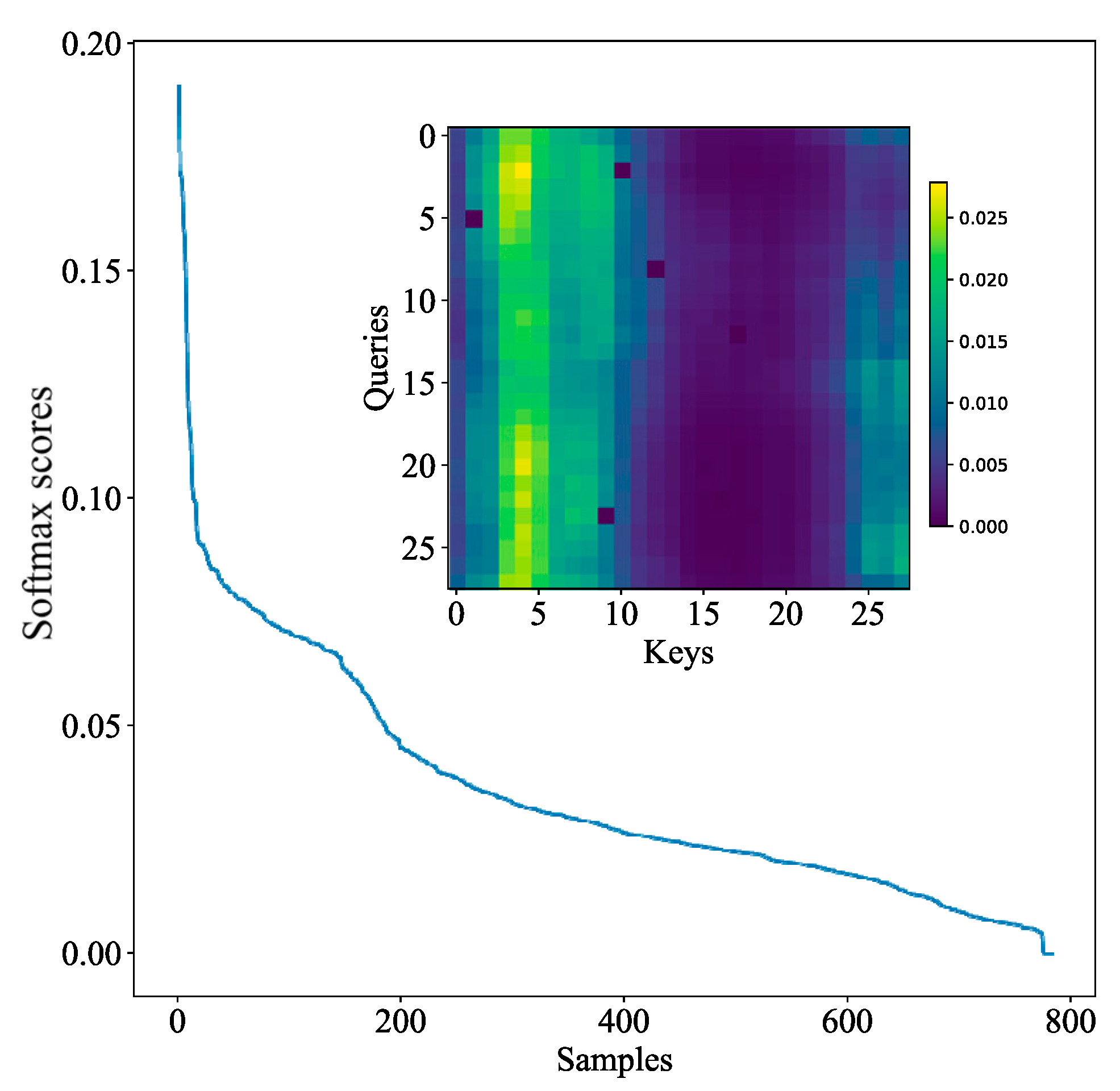
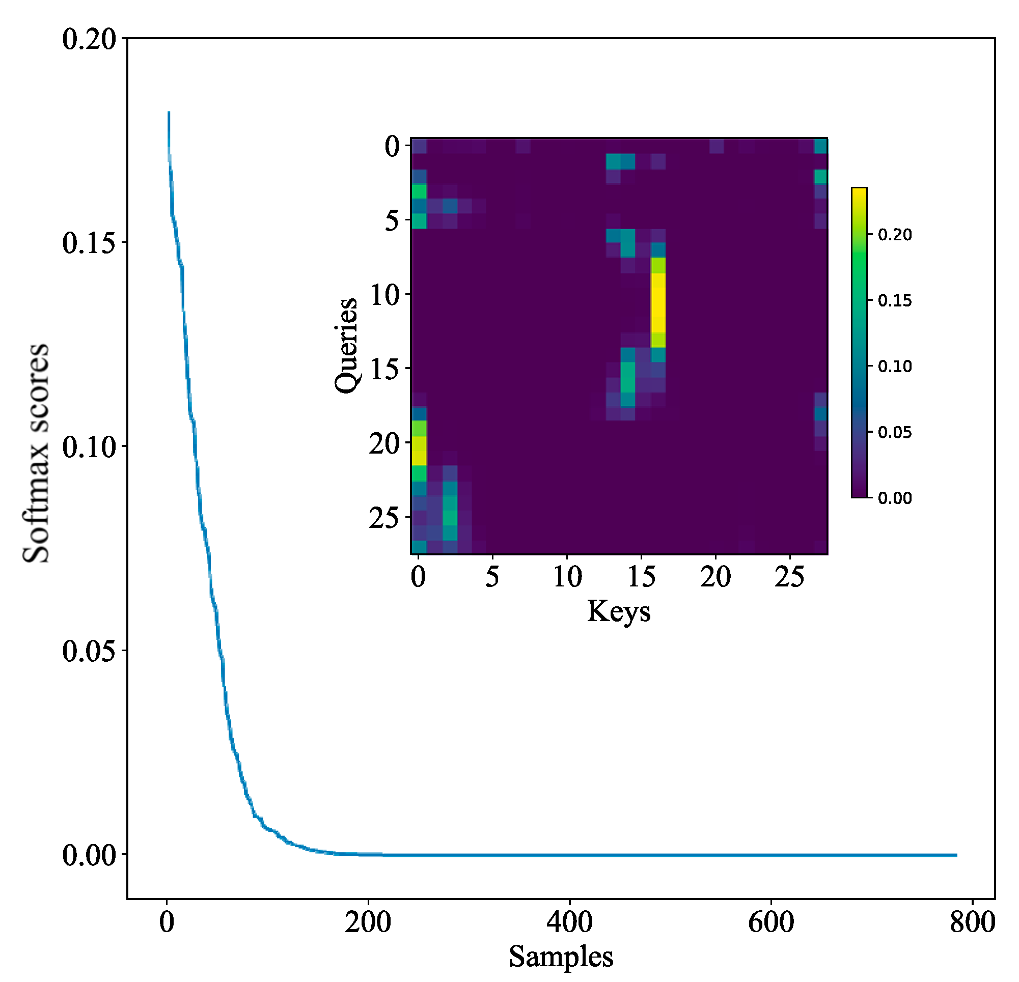
4.5. Visualization of Self-Attention
This paper presents a visual experiment of the ProbSparse attention mechanism. In the attention, we expect that the attention distribution varies greatly, and each
can focus on the relevant
, rather than obeying uniform distribution.
Figure 9 and
Figure 10 show the distribution maps of full self-attention and Probsparse self-attention, respectively. Each distribution consists of a curve and a heat map, corresponding to the self-attention of the encoder. The heat map shows the attention relationship between each
and each
. The greater the attention value, the higher the correlation, and the more important the feature. Comparing the two heat maps, it can be seen that the Probsparse self-attention feature is more obvious and less than the full self-attention, thereby reducing the calculation. The curve shows the distribution of each attention point. In fact, self-attention features both obey a long-tail distribution, and Probsparse self-attention is more obvious, so lazy attention with a small value is ignored, and only active attention with a large value is extracted.
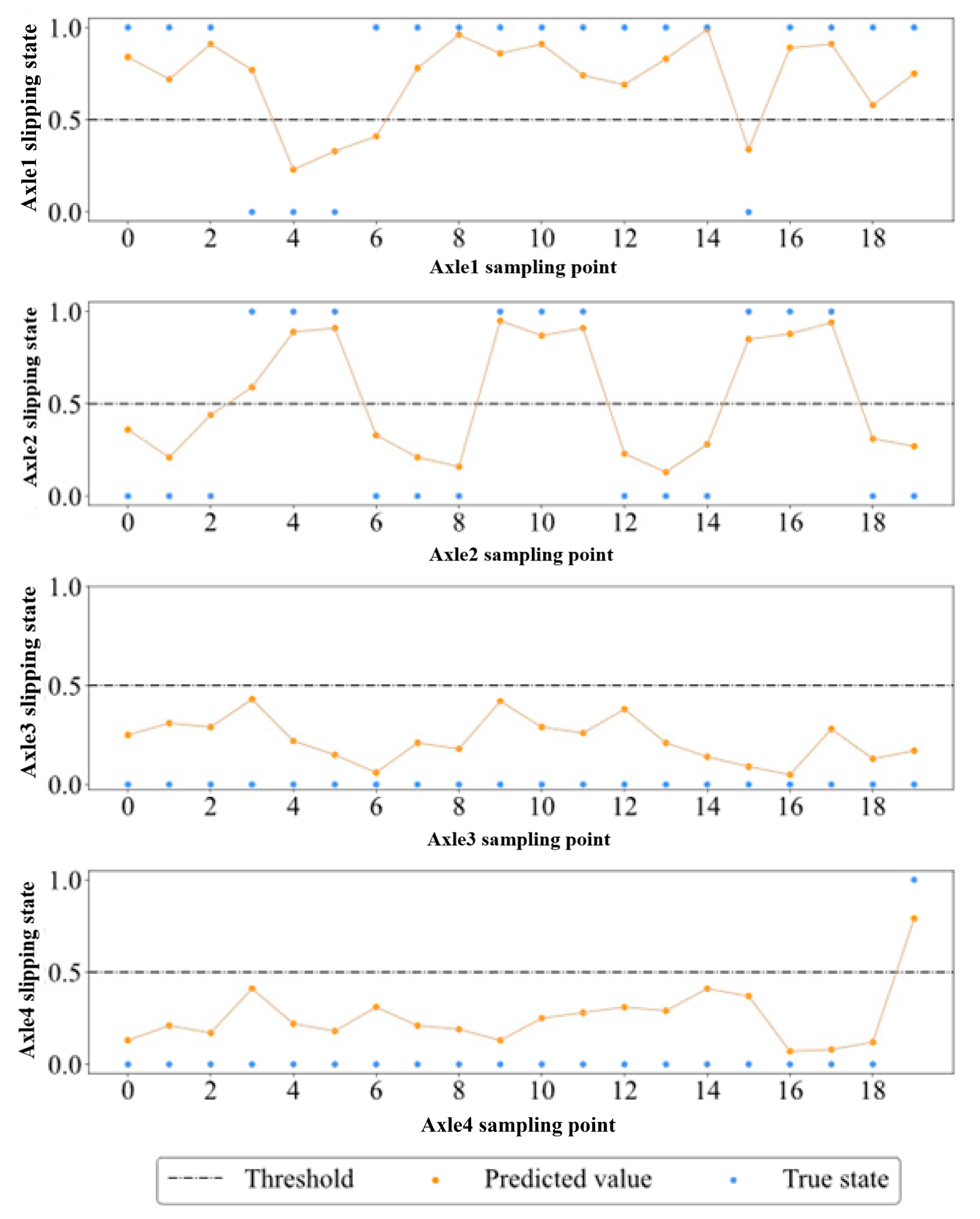
4.6. Display of Practical Forecast Effect
We screened a real sequence of four axle slipping states in the test set. As can be seen from
Figure 11, our model has a good prediction effect and few continuous prediction errors, and can predict the slipping state n steps ahead. In actual locomotive control, even if torque misadjustment caused by a prediction error occurs, it can be corrected immediately in the next cycle. Therefore, on the whole, this misprediction will not affect the adhesion utilization, but if real slipping can be predicted in time, it will improve adhesion utilization.
4.7. Experimental Configuration and Model Structure
The GPU used in the experiment was the NVIDIA GeForce RTX 3080 (NVIDIA, Santa Clara, CA, USA), and the CPU used was the 12th Gen Intel(R) Core(TM) i5-12600KF (Intel, Santa Clara, CA, USA). As shown in
Table 5, A total of 20,788 parameters needed to be trained, with a memory footprint of about 230 MB. Each prediction step took 4.45 ms on the CPU, or 3.11 ms on the GPU. In the actual locomotive control, a control cycle of about 10 ms. Therefore, both CPU-based and GPU-based detection speed can meet the system requirements.
5. Conclusions
This paper proposes a novel slipping classification prediction method and describes its related adhesion characteristics, improved Informer algorithm, and self-attention mechanism. Based on the Informer regression prediction model, this method improves the input and output structure of the model, so as to classify and predict the slipping state. In this study, relative position embedding was used to process the input data to enhance the timing information. This method was proven to be effective through a large number of experiments. Compared with the traditional model, it has the following improvements:
- (1)
The proposed model can output several steps at the same time, and has a high accuracy and recall rate.
- (2)
The detection speed is superior to that of other models, and it takes 3.11 ms for each forward propagation, meaning that the model can be used for online prediction.
- (3)
This model can simultaneously predict the multi-axle slipping state of the locomotive, and the comprehensive index is good. The highest accuracy rate reaches 94.75%, the recall rate reaches 91.23%, and the F1 reaches 92.67%.
- (4)
This paper considers some parameters which affect the slipping state and are difficult to analyze, such as the shaft speed, inverter voltage, and current.
Therefore, compared with traditional methods, the method proposed in this paper is significantly improved in all aspects. Through many experiments on a large amount of data, it has been proven that the improved Informer model is effective in slipping detection.
The method proposed in this paper was developed under ideal conditions. However, in actual operation, traction control is implemented through the motor, and current control methods output ideal motor torque commands. In practice, the motor torque output is subject to certain disturbances and fluctuations, which may affect the controller’s performance. Future research will further explore this issue by conducting joint experiments incorporating a motor model and a train model, based on the current framework. If possible, real-world vehicle tests will also be conducted.


