Featured Application
This study presents the application of a pulsed DC excitation method to improve the reliability of resistive frost-detection sensors by minimizing electrochemical reactions caused by a continuous electric field in water. These sensors can be integrated into evaporators in refrigeration systems, where frost detection enables optimized defrost demand strategies, enhanced defrost cycle efficiency, reduced energy consumption, and increased maintenance quality for stored products.
Abstract
Demand defrosting is a well-established strategy for improving defrost efficiency in refrigeration systems, and resistive frost-detection sensors provide a cost-effective means of enabling such control. However, copper electrode resistive sensors operating in water-based environments are susceptible to electrolysis, which degrades electrode integrity and compromises measurement reliability. This study investigates the impact of electrolysis on sensor performance and evaluates the effectiveness of an intermittent powering method in mitigating these effects. Two sensor excitation methods were experimentally tested: continuous voltage application and pulsed DC excitation with a 1.7% duty cycle. The results demonstrated that continuous excitation caused erratic measurements and electrode degradation due to ongoing electrochemical reactions. In contrast, the pulsed DC excitation method stopped observable electrolysis effects, leading to stable measurements and improved sensor longevity. These findings highlight pulsed DC excitation as a practical and effective solution for enhancing the accuracy and durability of resistive frost-detection sensors, making them more suitable for long-term use in commercial refrigeration system evaporators.
1. Introduction
Energy efficiency is most relevant in modern engineering, driven by environmental concerns and the need to reduce operating costs in large-scale applications. In refrigeration systems, frost accumulation on heat exchangers diminishes heat transfer efficiency, resulting in increased energy consumption [1]. Frost forms when air with a dew point above the surface temperature of the heat exchanger comes into contact with its subfreezing surfaces. This leads to water vapor deposition and subsequent freezing, creating a porous frost layer composed of ice crystals and trapped air. Over time, this layer grows and acts as thermal insulation, decreasing the heat exchanger’s efficiency. In severe cases, frost can block airflow, causing system malfunction [2].
Defrosting addresses the issue by actively removing the accumulated frost from the heat exchangers. Techniques such as electrical heating, hot gas bypass, and reverse-cycle defrosting melt and dislodge the frost, thereby restoring effective heat transfer and returning the system to normal function [3].
Traditional defrosting methods typically operate on preset time intervals without considering the actual frost buildup in the system [4]. This approach assumes a uniform rate of frost formation; however, variations in ambient temperature, humidity, and system load often lead to differences in frost accumulation [5]. As a result, defrost cycles are often triggered either too early, when frost levels are too low to impact performance, or too late, after excessive frost buildup has already degraded efficiency for an extended period. This leads to overall system inefficiency, unnecessary energy expenditure, and thermal disturbances within the refrigerated chamber. In contrast, demand defrost strategies employ real-time frost detection to trigger defrost cycles only when needed [6]. This minimizes wasted energy by defrosting solely in response to actual frost accumulation. Moreover, by synchronizing the defrost cycle with the true condition of the heat exchanger, demand defrost contributes to maintaining a more stable temperature environment within the refrigeration system. Traditional methods often cause unnecessary periodic warming, which exposes refrigerated products to cyclic temperature fluctuations. These fluctuations can accelerate quality degradation and reduce shelf life, whereas demand defrost, by reducing the amount of defrost cycles to the strictly necessary, helps preserve the freshness and quality of perishable items [4].
Demand defrost technologies can detect, predict, or measure frost accumulation. Prediction methods are based on computational models and machine learning algorithms to forecast frost formation based on environmental and operational data [7]. Detection methods are categorized into indirect approaches, which monitor ambient conditions such as temperature, humidity, refrigerant temperature, airflow, or pressure drops [8], and direct approaches, which use sensors to directly measure frost buildup [9].
There are several types of frost-detection sensors used in direct measurement approaches. Capacitive sensors detect frost by measuring variations in dielectric properties between water, air, and ice [10]; optical sensors use infrared- or laser-based techniques to detect frost accumulation by analyzing light reflection or absorption [11]; piezoelectric sensors determine frost thickness by measuring changes in resonance frequency, which directly correlates with frost thickness [12]. Image-processing techniques use cameras and machine vision algorithms to detect frost patterns on heat exchanger surfaces [13,14,15], and resistive sensors measure changes in electrical resistance as frost accumulates on the sensor surface [16,17,18]. These resistive sensors are simple, cost-effective, and sufficiently reliable for frost detection.
Working Principles of a Resistive Frost-Detection Sensor
Resistive frost-detection sensors function based on the principle of electrical resistance variation between two electrodes. In previous research, copper electrodes were arranged in a configuration where their resistance changes depending on the medium present between them. This operating principle is illustrated in Figure 1.
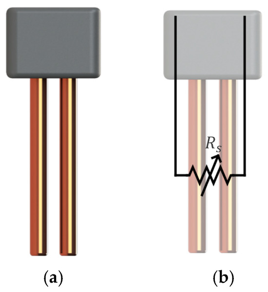
Figure 1.
Simplified diagram of the resistive frost-detection sensor (a) and overlaid equivalent circuit representation highlighting the sensor’s variable resistance (b) [17].
The resistivity of the medium between the electrodes is influenced by the presence of air, water, or frost. As condensation or frost forms, the medium’s electrical properties change, altering the overall sensor resistance. By measuring these variations, it becomes possible to infer the presence of moisture or frost accumulation on the surface of a heat exchanger (HX). Prior studies [16] have shown that a copper wire electrode sensor with a fabric medium provided superior performance in frost detection compared to other resistive sensor designs. A visualization of this sensor is presented in Figure 2.
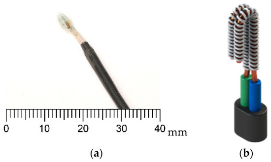
Figure 2.
Resistive frost-detection sensor with a fabric medium between the electrodes (a) and a rendered model (b) of this sensor as developed in [16].
Sensor resistance measurements were obtained using a voltage divider circuit, as shown in Figure 3, which converts variations in the sensor’s resistance into a measurable output voltage.
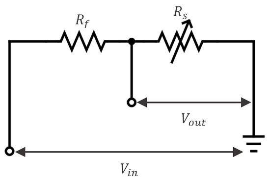
Figure 3.
Voltage divider circuit, with as the fixed resistor, as the sensor’s variable resistance, and and as input and output voltages, respectively.
The variable resistance of the sensor () results from changes in the electrical properties of the medium between the electrodes, which may consist of air, water, or frost/ice. These variations can be further influenced by factors such as frost density, water purity (distilled or ion-rich), and the presence of other impurities. This affects the output voltage as given by Equation (1):
where is the output voltage , is the input voltage , is the variable resistance of the frost measuring sensor , and is a fixed resistance .
By measuring , the value of can be calculated by solving Equation (1) for , as shown in Equation (2):
The voltage divider was powered by a 5 V supply, connected between VCC and GND, with fed into a 10-bit analog-to-digital converter (ADC) for data acquisition. Since is continuously supplied, an electric field is always present across the sensor electrodes, regardless of whether the ADC is actively reading.
As a result, the negatively charged electrode acts as a cathode, while the positively charged electrode functions as the anode. In the presence of an electric field, water molecules that are condensed between the sensor electrodes dissociate, initiating electrochemical reactions at each electrode.
At the cathode, a reduction reaction occurs, where water molecules gain electrons, producing hydrogen gas (H2) and hydroxide ions (OH−), as described by Equation (3):
Simultaneously, at the anode, an oxidation reaction takes place, where water molecules lose electrons, leading to the formation of oxygen gas (O2) and hydrogen ions (H+), as shown in Equation (4):
These electrochemical reactions generate ions that increase the conductivity of the water and lead to the production of hydrogen and oxygen gases at the electrodes. This effect impacts the electrical resistance measurements, making the use of a resistive sensor less reliable in such conditions. Therefore, understanding the ionic processes occurring at the sensor electrodes is essential to improve measurement reliability.
Even in the absence of an external electric field, H+ and OH− ions naturally exist in small, equal concentrations in distilled water due to the self-ionization of water molecules, as described by Equation (5):
However, when a voltage is applied across the sensor, ion migration occurs. Although distilled (or condensed) water contains very few free ions due to its high purity, the applied electric field induces the movement of these ions. ions migrate toward the cathode, where they gain electrons and form hydrogen gas, as described by Equation (6):
Conversely, ions migrate toward the anode, where they lose electrons, producing water and oxygen gas, as shown in Equation (7):
While positive and negative ions migrate in opposite directions within the medium, they typically do not recombine into water under the influence of the applied electric field, instead forming an ionic current between the electrodes. However, once the electric field is removed, their inherent charge attraction becomes dominant in the absence of the external electric field and these ions will naturally recombine to form water.
A common approach to reducing long-term electrochemical effects of electrolysis in resistive sensors is using alternating current (AC) excitation [19,20], where the voltage applied to the sensor terminals is cyclically reversed at a determined frequency. This neutralizes the electrochemical effects accumulated during the previous cycle, preventing charge buildup and unwanted ion migration. Another method is pulsed DC excitation [21], in which the sensor is powered intermittently with controlled pulse durations, minimizing the duration of electrolysis while allowing ions to recombine between pulses, and thereby reducing charge buildup and mitigating long-term electrochemical effects.
Other approaches to mitigating electrolysis effects include sensor designs that minimize the electric field intensity by increasing electrode spacing, using interdigitated geometries, or the inclusion of neutral or guard electrodes, helping to reduce unintended electrochemical reactions [22]. However, the goal of this study is to explore control-based strategies to mitigate the electrolysis effects observed in sensors designed and tested in previous works. Sensor design modifications will only be considered if these methods prove to be insufficient in addressing the issue.
While AC excitation is effective, it typically requires additional circuitry. In contrast, pulsed DC excitation can be implemented using standard microcontroller-based systems without requiring modifications to the existing hardware.
Given that the sensor infrastructure developed in previous studies [16,18] was based on DC measurement techniques, pulsed DC excitation was selected for this study. It offers simplicity, ease of integration, and reduces electrolysis effects while maintaining compatibility with the existing system architecture.
2. Materials and Methods
To investigate the effects of a pulsed DC excitation control method, an experiment was designed using two identical resistive sensors. One sensor served as the control, using the same continuously powered measurement method as in previous studies [16,18], while the other implemented a pulsed DC excitation method. To ensure consistency with prior research, the sensor acquisition rate was maintained at 3 s intervals, preserving the same measurement conditions.
2.1. Control Method
The two sensors were subjected to different measurement methods. The first sensor, serving as the control, was continuously powered, replicating the reading method used in previous studies [16,18]. The second sensor utilized a pulsed DC excitation method, in which a pulse-width-modulated (PWM) signal was used to periodically apply voltage, controlling the duration and frequency of excitation. Figure 4 illustrates a PWM waveform applied to the on the second sensor:
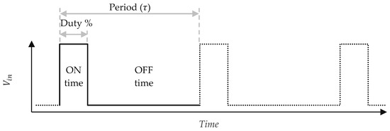
Figure 4.
PWM-based pulsed DC excitation waveform applied to the second sensor.
Measurements are taken every three seconds, as this was the measurement period used in previous studies [16,18]. The sensor is powered for 50 ms per cycle as this was found to be the minimum time for the voltage across the sensor electrodes to stabilize and for the measurement to be recorded. This results in a 1.7% duty cycle, meaning the sensor in the PWM-based method is powered for only 1.7% of the time compared to the continuously powered sensor in the control setup.
2.2. Data Acquisition
The sensors were connected to a 10-bit ADC and employed two distinct sensor excitation methods: continuous DC voltage and pulsed DC excitation. These are illustrated in Figure 5. For the continuous DC voltage method, represented in Figure 5a, was directly connected to the microcontroller’s VCC and GND, continuously supplying the sensor electrodes with a constant voltage while monitoring the resulting current. In contrast, the pulsed DC excitation method, represented in Figure 5b, involved connecting to a digital output (DO) and GND of the microcontroller.
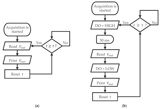
Figure 5.
Flowchart representation of the two sensor acquisition methods, with continuous DC excitation (a) and pulsed DC excitation (b).
The DO acted as a controlled power source, supplying power to the sensor for 50 ms, which is sufficient for performing the measurement; subsequently, it was turned off for the remaining 2950 ms within each 3 s cycle. Consequently, measurements occurred intermittently at approximately 0.33 Hz, with a duty cycle of about 1.7%. This method aimed to minimize electrode polarization effects. Both excitation methods utilized an identical voltage of 5 V to allow for a direct comparison of sensor responses under comparable environmental conditions.
This can be represented by Equation (8) for continuous DC excitation:
And by Equation (9) for pulsed DC excitation method:
In both cases, the measured values were transmitted via serial communication to MATLAB 2018b, where they were plotted in real-time and logged into a CSV file for further analysis. To enable a direct comparison between the two methods in this experiment, the sensors were designed to operate both in view and outside the refrigeration system, ensuring controlled observation of their behavior under different conditions. The test was conducted for 5 h and 45 min.
2.3. Sensor Design and Configuration
Each sensor was enclosed within a sealed glass flask filled with distilled water and consisted of two parallel copper electrodes, each measuring 35 mm in length and 2.25 mm in diameter, with a 5 mm separation distance between them. The electrodes were fully submerged in distilled water, which was chosen as a medium to represent the condensed water formed inside the HX during operation. The sensor configuration is illustrated in Figure 6.
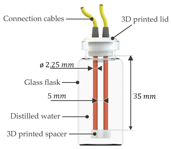
Figure 6.
Rendered front view of the individual sensor configuration.
The two flask-encased sensor electrodes were mounted onto a nonconductive 3D-printed jig consisting of a lid and a spacer. Figure 7 shows the two sensors. The sensor on the right, connected via blue cables, was operated under the continuous-power approach and remained constantly powered throughout the experiment. Conversely, the sensor on the left, connected via green cables, utilized the pulsed DC excitation method, in which was pulsed to assess the potential benefits of intermittent excitation in reducing electrochemical effects.
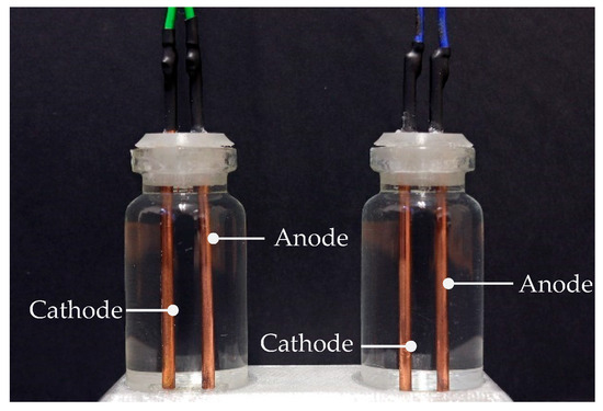
Figure 7.
Sensor configuration, showing the two sensors, subjected to the continuous reading method (right) and pulsed DC excitation method (left).
The sensors were intentionally designed to be larger than the application size to enhance visualization of electrochemical reactions during the experimental analysis. While previous studies have focused on miniaturization by using smaller electrodes [16,17], the larger electrode dimensions in this study allow for better observation of potential electrochemical effects.
Copper was chosen as the electrode material as it was the material used in previous studies [16,18]. It was chosen because it has good electrical conductivity, is widely available and cost-effective, and can be easily shaped and soldered. While copper is not as resistant to electrochemical reactions as noble metals, its behavior under an electric field depends on environmental conditions. In distilled water, significant reactions are not expected in the absence of voltage. However, when an electric field is applied, electrochemical migration and oxidation can occur [23], degrading the electrode material.
If the sensor were to be implemented in a long-term application where electrode degradation became a concern, plating or the use of noble metals such as platinum or gold could be considered to mitigate these effects, as their high electrochemical stability and resistance to oxidation help prevent degradation and improve performance over time. This would mitigate electrochemical reactions involving the electrodes themselves, limiting the system’s behavior to water electrolysis only (Equations (3)–(7)), without electrode oxidation or material loss.
2.4. Acquisition Circuit
The sensor readings were acquired simultaneously under the same environmental conditions. This was performed using a voltage divider circuit, as shown in Figure 3, which, as previously discussed, converts variations in the sensor’s resistance into a measurable voltage signal. A fixed resistor, , of 2.7 kΩ was selected despite the sensor’s initial measured resistance of 16 kΩ. This choice was made because the conductivity of distilled water is expected to increase significantly over time due to electrochemical reactions occurring at the electrodes. While distilled water has very low ionic content and high resistance, the presence of dissolved ions in water significantly lowers resistance by increasing conductivity. As these reactions progress, ion concentrations in the water will rise, leading to a decrease in the sensor’s resistance, making 2.7 kΩ a more suitable fixed resistor value to maintain an optimal voltage range for measurement.
To analyze potential electrochemical effects, a camera was positioned in front of the sensors, programmed to capture images at 5 min intervals. This visual data complemented the electrical measurements, providing additional insight into the formation of electrochemical byproducts and changes in electrode appearance over time. The collected data helped assess the effectiveness of pulsed DC excitation in mitigating electrochemical effects, guiding potential improvements for future sensor implementations.
2.5. Data Analysis
To statistically analyze the stability differences between continuous and pulsed DC excitation methods, resistance measurements obtained from both methods were compared. Each sensor was measured repeatedly over equivalent intervals under the same environmental conditions. To quantify the differences in measurement stability, mean, variance, and standard deviation were calculated for each method. The coefficient of variation was also determined to compare the relative dispersion between datasets with different mean values. A paired-sample t-test was then applied to determine whether the observed differences between paired measurements were statistically significant. The paired-sample t-test compares two related samples and is defined by Equation (10):
where is the average difference between pairs, is the standard deviation of the differences, and is the number of paired observations.
Additionally, measurement instability was quantified by comparing the variance of resistance measurements. Electrode degradation was assessed visually through high-resolution photography, identifying surface changes indicative of electrochemical degradation.
2.6. Image-Based Quantification of Electrode Deposits
To complement visual observations and resistance measurements, a computer vision tool was developed in Python 3.11.9 using OpenCV 4.11.0 to quantify the visual accumulation of electrochemical byproducts on the sensor electrodes over time. The analysis was based on time-lapse images taken during the experiment.
For the left electrode, which accumulated a black deposit, grayscale image analysis was applied. Each image was cropped to focus on the electrode region, and contrast enhancement was performed using CLAHE (Contrast-Limited Adaptive Histogram Equalization). The number of pixels below a fixed intensity threshold (grey level < 25) was then counted to estimate the amount of black material deposited on the electrode surface.
For the right electrode, which developed a blue precipitate attributed to copper hydroxide, color filtering was used to isolate the deposit. After image cropping and contrast enhancement, red-dominant and black areas were masked out. The remaining pixels were counted to approximate the area covered by the blue substance
These image-based metrics provided a method to track the visual progression of material accumulation on each electrode throughout the experiment.
3. Results
The experiment was conducted over a 5 h and 45 min period. Both sensors were subjected to a 5 V excitation: the continuous sensor remained constantly powered, while the pulsed sensor received 5 V for 50 ms every 3 s. To streamline analysis and improve result visualization, the recorded data were post-processed to a 60 s interval, filtering out redundant measurements. As shown in Figure 8, the results reveal a clear distinction between the two sensor measurement methods.
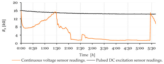
Figure 8.
Comparison of measurement results between continuous voltage sensor readings and pulsed DC excitation sensor readings.
The measurements obtained using the continuously powered sensor method were highly erratic; the resistance values fluctuated unpredictably between a maximum of 16.0 kΩ and a minimum of 1.4 kΩ. The curve exhibited irregular, sharp drops and jumps, showing considerable instability throughout the measurement process.
In contrast, the pulsed DC excitation sensor reading method produced a much more stable curve, displaying a concave downward shape with a decreasing slope. The resistance started at 16.1 kΩ and gradually decreased to 14.4 kΩ, where it stabilized. This behavior occurs because, although the duty cycle is very low, the brief application of voltage is sufficient to increase ion presence, reducing water resistivity. However, due to the reversible nature of the reaction (as shown in Equation (5)), the resistivity decline eventually levels off as equilibrium is reached between ion formation during the 50 ms pulses and ion recombination (neutralization).
As seen in Figure 9, during testing with the pulsed DC excitation method, no visible changes occurred in the electrodes or the water; this outcome is consistent with the experiment’s objectives.
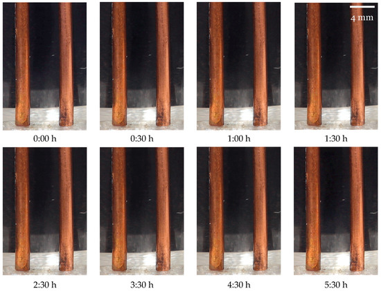
Figure 9.
Sensor electrodes during testing for the pulsed DC excitation method.
It should also be noted that in the top row of Figure 9, from to , the time interval between pictures is , whereas in the bottom row, from to , the interval is . The timestamps are also marked in the graph of Figure 8 with vertical dashed bars to facilitate the analysis. The results from the continuously powered sensor reading method reveal markedly different outcomes, as shown in Figure 10.
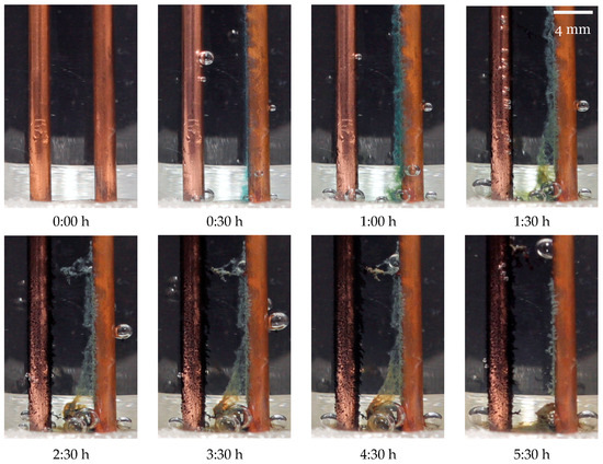
Figure 10.
Sensor electrodes during testing for the continuously powered sensor reading method.
Multiple electrochemical reactions occur both at the electrodes and within the water, developing over time as shown in Table 1.

Table 1.
Observations in electrodes during testing for the continuously powered sensor reading method.
It should again be noted, as seen in Figure 9, that, for the images in the top row of Figure 10 from to , the time interval between pictures is 0:30 h, whereas in the bottom row, from to , the interval is .
The progression of dark material accumulation on the cathode was quantified based on the percentage of black pixels in the corresponding image region. These values are plotted in Figure 11 for both excitation methods. The results are coherent with the images, as the subjected to continuous excitation exhibited a sharp increase in black pixel percentage after , which consistently increased up to when the images confirm that the growth had stabilized. In contrast, the sensor excited using 50 ms pulses showed a much lower and more stable percentage of black pixels throughout the test duration.
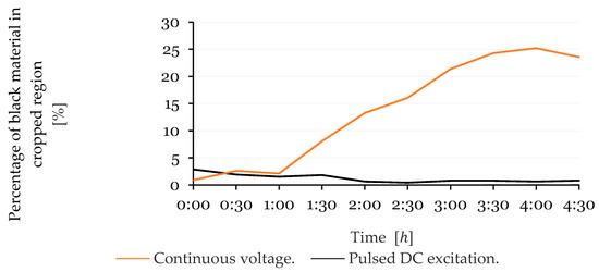
Figure 11.
Percentage of black pixels in the cropped cathode region over time for the continuous DC excitation powered sensor and the pulsed DC excitation method.
The accumulation of blue material on the anode was quantified based on the percentage of remaining non-black and non-red pixels in the cropped image region. Figure 12 presents the evolution of this value over time. In the sensor powered using the continuous DC excitation method, the percentage of blue material increased sharply up to and after this, a stabilization, or even slight decrease trend, was observed. In contrast, the sensor subjected to the pulsed DC excitation method exhibited lower and relatively stable values, with no evident accumulation trend.
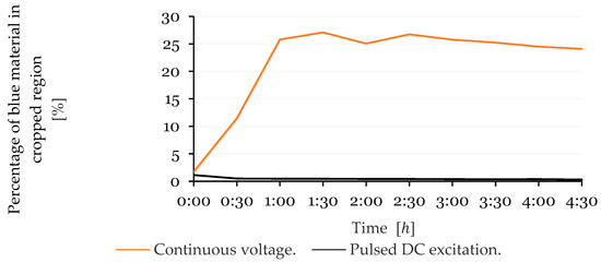
Figure 12.
Percentage of detected blue material in the anode region over time for the sensor powered using the continuous DC excitation method and the sensor operated with the pulsed DC excitation method.
These electrochemical reactions and their impacts on sensor measurements can now be compared to the sensor-measured data of Figure 8, noticing the timestamps marked by the vertical dashed bars in the figure to facilitate analysis.
4. Discussion
To clarify the differences in measurement behavior between excitation methods, key statistical indicators—mean, standard deviation, coefficient of variation, and variance—were calculated for both datasets. The pulsed method yielded a mean resistance of 14.77 kΩ, with a standard deviation of 0.47 kΩ and a coefficient of variation of 3.17%, indicating a stable and consistent measurement profile. In contrast, the continuous excitation method produced a lower mean of 5.11 kΩ, but with a much higher standard deviation of 4.34 kΩ and a coefficient of variation of 84.97%, reflecting significant fluctuation and instability in the signal. The variance values reinforce this distinction: 0.22 kΩ2 for the pulsed method versus 18.83 kΩ2 for the continuous method. These metrics demonstrate that pulsed excitation leads to more consistent readings with reduced noise, while continuous excitation results in higher dispersion, potentially due to progressive electrode degradation or polarization effects. A summary of the descriptive statistics for both methods is presented in Table 2.
Table 2.
Descriptive statistics for resistance measurements under different excitation methods.
A paired-samples t-test was also performed to analyze the significance of the differences observed between the two excitation methods. The test compared paired resistance values collected simultaneously from both the pulsed and continuous excitation methods. The resulting t-statistic was 196.50, with a p-value below 0.001, indicating a significant difference between the two datasets. This result confirms that the differences in mean resistance values are not due to random variation but are statistically meaningful. The t-test thus reinforces the findings already evident from the variance, standard deviation, and coefficient of variation, confirming the improved stability of the pulsed excitation method.
Unstable measurements were also visibly identified by high amplitude fluctuations and abrupt resistance variations observed in Figure 8, supporting the statistical results.
Visual inspection through high-resolution photography further indicated electrode degradation associated mostly with continuous DC excitation, evidenced by apparent electrochemical degradation.
In addition to qualitative observations, Figure 11 and Figure 12 provide a quantitative perspective on electrode surface changes by tracking the accumulation of black and blue materials over time. The percentage of black pixels, associated with material buildup on the cathode, increased sharply in the sensor powered by the continuous DC excitation method, peaking at 25% by , whereas the sensor subjected to the pulsed DC excitation method maintained a low and stable level below throughout the test.
Similarly, the anode showed a progressive increase in the percentage of non-black and non-red pixels—corresponding to blue material—in the continuous DC excitation condition, reaching over 27% at the peak. The pulsed DC method again demonstrated more stable results, with percentages remaining below 3%. The slight decrease in values observed toward the end for the electrodes powered using the continuous excitation method is attributed to the precipitation of the formed substances outside the cropped region analysed for this method.
The result analysis is based on the understanding that the materials involved are copper and distilled water subjected to an electric field.
Based on the observed colors of the materials deposited on the sensor electrodes—black and blue—two compounds are identified as the likely candidates. The black material is copper(II) oxide (), while the blue material is copper(II) hydroxide (). These observations help explain the electrochemical phenomena occurring during the experiment, as detailed below:
- The cathode acquires a polished, reflective surface:
As the electrodes were previously exposed to air, a thin layer of Cu2O (Copper(I) oxide) is present on both the electrodes. When the sensor is powered, electrons flow into the anode, facilitating a reduction reaction, as described by Equation (11):
Since copper without an oxide layer has a polished, metallic appearance, this reaction results in a reflective surface.
- The presence of copper(II) hydroxide, Cu(OH)2, and copper(II) oxide, CuO:
When noble metals are used as electrodes, only and ions migrate between the anode and cathode. However, when copper electrodes are used, oxidation at the anode occurs, and ions form, as shown in Equation (12):
These copper ions migrate toward the cathode, where they are expected to gain electrons and form copper again. However, upon encountering ions, they react to form , as described in Equation (13):
This reaction occurs at both electrodes. Near the anode, ions form and migrate toward the cathode, while ions form at the cathode and migrate toward the anode. Due to the low voltage and current ( and , respectively), there is a higher concentration of ions near the cathode and ions near the anode.
can remain stable in pure water without transforming into . However, in the presence of ions (as in alkaline solutions), this transformation occurs more rapidly [24]. Under these conditions, copper ions dissolve, forming , which eventually leads to the formation of , as described in Equation (14):
This explains the presence of copper(II) hydroxide near the cathode and copper(II) oxide near the anode.
- Oxygen () and hydrogen () gas bubbles:
Gas bubbles formed from oxygen and hydrogen are expected, as explained in the water electrolysis reactions given in chemical Equations (3), (4), (6), and (7). However, the observed oxygen production is visually lower than expected, likely due to the disproportionate consumption of oxygen molecules in the formation of and .
These reactions are the key chemical processes observed during the experiment. With this understanding, the behavior of the curve in the continuous voltage sensor readings, shown in Figure 8, can be explained as shown in Table 3:
Table 3.
Explanation for the observations made in the electrodes during testing for the continuously powered sensor reading method.
This explanation highlights the dynamics of continuous monitoring and its impact on electrode degradation, as the anode loses copper ions during electrolysis, accelerating the deterioration process. The experiment demonstrates how the control method directly affects sensor reliability and emphasizes the need to account for the effects of electrolysis when using a resistive sensor in a water medium. The pulsed DC excitation control solution addresses this issue by minimizing the duration in which electrolysis occurs between the sensor electrodes.
5. Conclusions
The comparative analysis between continuous and pulsed DC excitation methods revealed clear advantages of the pulsed approach regarding measurement stability and electrode preservation. Descriptive statistics—mean, standard deviation, coefficient of variation, and variance—were used to evaluate performance. Pulsed DC excitation yielded significantly lower variance, standard deviation, and coefficient of variation, indicating more consistent and reliable sensor performance under the same environmental conditions. The mean resistance for the pulsed method was 14.77 kΩ, with a standard deviation of 0.47 kΩ and a coefficient of variation of 3.17%, in contrast to the continuous method’s 5.11 kΩ mean, 4.34 kΩ standard deviation, and 84.97% coefficient of variation. Variance further highlighted this difference, with 0.22 kΩ2 for pulsed versus 18.83 kΩ2 for continuous excitation. The paired-samples t-test further confirmed the statistical significance of these differences (t = 196.50, p < 0.001).
Moreover, the continuous excitation method exhibited visual signs of electrode degradation, while the pulsed method did not. This was achieved by limiting voltage application to short intervals (50 ms ON time) with a 1.7% duty cycle for an acquisition rate of 0.33 Hz. The pulsed DC method significantly reduced electrolysis effects, preventing the visible formation of and gas, and ions, as well as copper(II) hydroxide (Cu(OH)2) and copper(II) oxide (CuO) deposits. This reduction in electrochemical byproducts also helped maintain electrode integrity, ensuring more stable and reliable sensor operation.
The degradation effects were further confirmed through quantitative image analysis. Measurements of dark material accumulation on the cathode (black pixels) and blue substance formation on the anode (remaining non-black/non-red pixels) supported the visual inspection. In both cases, the sensor powered using the continuous DC excitation method exhibited a clear increase in deposition over time, while the pulsed DC excitation method maintained consistently low values.
Although the pulsed DC excitation method caused some resistance changes, these were gradual and predictable, making it suitable for integration into demand defrost systems. In contrast, the continuous voltage method produced erratic fluctuations, introducing noise that could result in false-positive or false-negative readings in automated systems. While the pulsed DC method still led to some decrease in resistivity, the magnitude of this change was relatively small compared to the highly dynamic nature of frost formation, defrosting, and condensation in evaporators. As a result, this introduces a minimal and likely acceptable margin of error, with a low impact on frost detection accuracy. Previous studies have shown that frost detection remains feasible even with continuous voltage measurement, despite its susceptibility to electrochemical effects.
The resistive sensor offers a cost-effective and scalable solution for frost detection in refrigeration systems, enhancing the efficiency of demand defrost systems by reducing unnecessary defrost cycles. The findings of this study contribute to the development of energy-efficient refrigeration technologies, as frost sensing ensures defrost cycles are activated only when necessary, minimizing the energy consumption associated with unnecessary defrosting operations while maintaining temperature stability. By improving the reliability and accuracy of frost detection, the proposed sensor can further optimize defrosting processes, reducing waste and enhancing energy efficiency in cold chain logistics.
Future studies could explore the use of noble metals to mitigate some of the adverse effects of electrolysis, as they do not release ions into the water during oxidation reactions. Additionally, integrating noble metals would have a minimal impact on sensor costs for the developed sensors. For example, platinum has a density of 21.45 g/cm3 and reached a 5-year price peak of EUR 34.56 on 6 February 2021 [25], yet the raw material cost per small electrode would still be below EUR 1. However, pulsed DC excitation remains essential, as even with non-reactive noble metals, electrolysis would still occur. The presence of dissolved and ions, along with the production of and gases accumulating near the electrodes destabilizes resistance readings. These effects make the continuous voltage approach unsuitable for long-term use in frost detection systems, regardless of the electrode material used.
Further work should examine the integration of resistive sensors into existing refrigeration control systems for automated frost detection and defrost initiation. The sensor’s simple electrical interface allows for direct compatibility with common microcontroller- or PLC-based platforms. Machine learning algorithms could enhance the sensor’s ability to differentiate between frost, water, and air under complex operating conditions.
Author Contributions
Conceptualization, M.L.A.; methodology, M.L.A., P.D.G. and P.D.S.; software, M.L.A.; validation, P.D.S.; formal analysis, M.L.A., P.D.G. and P.D.S.; investigation, M.L.A., P.D.G. and P.D.S.; resources, P.D.G.; data curation, M.L.A.; writing—original draft preparation, M.L.A.; writing—review and editing, P.D.G. and P.D.S.; supervision, P.D.S.; funding acquisition, P.D.G. All authors have read and agreed to the published version of the manuscript.
Funding
The authors would like to express their gratitude to Fundação para a Ciência e Tecnologia (FCT) and C-MAST (Centre for Mechanical and Aerospace Science and Technologies) for their support in the form of funding, under the project UIDB/00151/2020.
Institutional Review Board Statement
Not applicable.
Informed Consent Statement
Not applicable.
Data Availability Statement
The raw data supporting the conclusions of this article will be made available by the authors on request.
Acknowledgments
The authors acknowledge the support provided by LITecS (Laboratory of Innovation and Technologies for Sustainability) (https://litecs.ubi.pt/en/ accessed on 10 March 2025).
Conflicts of Interest
The authors declare no conflicts of interest.
References
- Krasota, D.; Błasiak, P.; Kolasiński, P. Literature Review of Frost Formation Phenomena on Domestic Refrigerators Evaporators. Energies 2023, 16, 2945. [Google Scholar] [CrossRef]
- Hermes, C.J.L.; Piucco, R.O.; Barbosa, J.R.; Melo, C. A study of frost growth and densification on flat surfaces. Exp. Therm. Fluid Sci. 2008, 33, 371–379. [Google Scholar] [CrossRef]
- Jeong, H.; Byun, S.; Kim, D.R.; Lee, K.-S. Power optimization for defrosting heaters in household refrigerators to reduce energy consumption. Energy Convers. Manag. 2021, 237, 114127. [Google Scholar] [CrossRef]
- Malik, A.N.; Khan, S.A.; Lazoglu, I. A novel demand-actuated defrost approach based on the real-time thickness of frost for the energy conservation of a refrigerator. Int. J. Refrig. 2021, 131, 168–177. [Google Scholar] [CrossRef]
- Chung, Y.; Na, S.-I.; Yoo, J.W.; Kim, M.S. A determination method of defrosting start time with frost accumulation amount tracking in air source heat pump systems. Appl. Therm. Eng. 2020, 184, 116405. [Google Scholar] [CrossRef]
- Malik, A.N.; Khan, S.A.; Lazoglu, I. A novel hybrid frost detection and defrosting system for domestic refrigerators. Int. J. Refrig. 2020, 117, 256–268. [Google Scholar] [CrossRef]
- Alcaraz, A.; Ilare, D.; Mansutti, A.; Cascini, G. Machine learning-based virtual sensors for reduced energy consumption in frost-free refrigerators. Proc. Des. Soc. 2024, 4, 1909–1918. [Google Scholar] [CrossRef]
- Maldonado, J.M.; de Gracia, A.; Zsembinszki, G.; Moreno, P.; Albets, X.; González, M.Á.; Cabeza, L.F. Frost detection method on evaporator in vapour compression systems. Int. J. Refrig. 2019, 110, 75–82. [Google Scholar] [CrossRef]
- Aguiar, M.L.; Gaspar, P.D.; Da Silva, P.D. Frost Measurement Sensors for Demand Defrost Control Systems: Purposed Applications in Evaporators; Springer eBooks: Berlin/Heidelberg, Germany, 2019; pp. 159–171. [Google Scholar] [CrossRef]
- Shen, Y.; Wang, S. Condensation frosting detection and characterization using a capacitance sensing approach. Int. J. Heat Mass Transf. 2019, 147, 118968. [Google Scholar] [CrossRef]
- Tai, Y.-H.; Kamal, A.S.A.; Park, Y.-J.; Tsai, P.-C.; Ho, Y.-L.; Wei, P.-K. Real-Time monitoring of Frost/Defrost processes using a tapered optical fiber. IEEE Sens. J. 2020, 21, 6188–6194. [Google Scholar] [CrossRef]
- Yang, Z.; Rupavatharam, S.; Burns, A.; Lee, D.; Howard, R.; Isler, V. Low-cost Refrigerator Frost Detection using Piezoelectric Sensors. In Proceedings of the ICC 2022—IEEE International Conference on Communications, Seoul, Republic of Korea, 16–20 May 2022; pp. 3530–3535. [Google Scholar] [CrossRef]
- Yuan, K.; Chen, J.; Liu, Y.; Lao, J. Research on frosting detection method of air source Heat pump based on vision Technology. J. Phys. Conf. Ser. 2022, 2354, 012017. [Google Scholar] [CrossRef]
- Zheng, H.; Jiang, S.; Wang, F.; Wang, X. Improving the accuracy of frosting image recognition for cold storage evaporators based on Gray-Level co-occurrence matrix and multi-layer Extreme learning Machine. In Proceedings of the 5th International Conference on Computer Information Science and Application Technology (CISAT 2022), Chongqing, China, 29–31 July 2022; pp. 347–354. [Google Scholar] [CrossRef]
- Aguiar, M.L.; Gaspar, P.D.; Da Silva, P.D. Image recognition method for frost sensing applications. Energy Rep. 2022, 8, 234–240. [Google Scholar] [CrossRef]
- Aguiar, M.L.; Gaspar, P.D.; Silva, P.D.; Silva, A.P.; Martinez, A.M. Medium materials for improving frost detection on a resistive sensor. Energy Rep. 2020, 6, 263–269. [Google Scholar] [CrossRef]
- Aguiar, M.L.; Gaspar, P.D.; Da Silva, P.D. Additive manufacturing of a Frost-Detection resistive sensor for optimizing demand defrost in refrigeration systems. Sensors 2024, 24, 8193. [Google Scholar] [CrossRef] [PubMed]
- Aguiar, M.L.; Gaspar, P.D.; Silva, P.D. Optimization and further experimental testing of a resistive sensor for monitoring frost formation in refrigeration systems. In Proceedings of the 6th IIR International Conference on Sustainability and the Cold Chain, Nantes, France, 26 August 2020; pp. 1–8. [Google Scholar] [CrossRef]
- Gillbanks, J.; Foster, K.; Sharma, P.; Keating, A.; Myers, M.; Nener, B.D. AC excitation to mitigate drift in ALGAN/GAN HEMT-Based sensors. IEEE Sens. J. 2023, 23, 12947–12952. [Google Scholar] [CrossRef]
- Zhao, W.; Zhang, H.; Zhang, J.; Zhang, L.; Zhou, S.; Zhou, H. Research and Design of Dual-Excitation Nine-Electrode Conductivity Sensor. In Proceedings of the 2023 IEEE 11th International Conference on Computer Science and Network Technology (ICCSNT), Dalian, China, 21–22 October 2023; pp. 286–292. [Google Scholar] [CrossRef]
- Kane, N.; Hartvigsen, J.; Casteel, M.; Priest, C.; Gomez, J.; Wang, L.; White, C.; Boardman, R.; Ding, D. Accelerated stress testing of standard solid oxide electrolysis cells. ECS Trans. 2023, 111, 2139–2146. [Google Scholar] [CrossRef]
- Bigharaz, M.; Schenkel, T.; Bingham, P.A. Increasing force generation in electroadhesive devices through modelling of novel electrode geometries. J. Electrost. 2020, 109, 103540. [Google Scholar] [CrossRef]
- Qi, K.; Huang, H. Electrochemical migration behavior of copper under a thin distilled water layer. Corros. Commun. 2023, 11, 52–57. [Google Scholar] [CrossRef]
- Cudennec, Y.; Lecerf, A. The transformation of Cu(OH)2 into CuO, revisited. Solid State Sci. 2003, 5, 1471–1474. [Google Scholar] [CrossRef]
- Platinum Price in EUR per Gram for the Last 5 Years. Bullionbypost. Available online: https://www.bullionbypost.com/platinum-price/5year/grams/EUR/ (accessed on 4 April 2025).
Disclaimer/Publisher’s Note: The statements, opinions and data contained in all publications are solely those of the individual author(s) and contributor(s) and not of MDPI and/or the editor(s). MDPI and/or the editor(s) disclaim responsibility for any injury to people or property resulting from any ideas, methods, instructions or products referred to in the content. |
© 2025 by the authors. Licensee MDPI, Basel, Switzerland. This article is an open access article distributed under the terms and conditions of the Creative Commons Attribution (CC BY) license (https://creativecommons.org/licenses/by/4.0/).