Impact of Texture Feature Count on the Accuracy of Osteoporotic Change Detection in Computed Tomography Images of Trabecular Bone Tissue

Abstract

The aim of this study is to compare the classification accuracy depending on the number of texture features used. This study used 400 computed tomography (CT) images of trabecular spinal tissue from 100 patients belonging to two groups (50 control patients and 50 patients diagnosed with osteoporosis). The descriptors of texture features were based on a gray level histogram, gradient matrix, RL matrix, event matrix, an autoregressive model, and wavelet transformation. From the 290 obtained texture features, the features with fixed values were eliminated and structured according to the feature importance ranking. The classification performance was assessed using 267, 200, 150, 100, 50, 20, and 10 texture features to build classifiers. The classifiers applied in this study included Naive Bayes, Multilayer Perceptron, Hoeffding Tree, K-nearest neighbors, and Random Forest. The following indicators were used to assess the quality of the classifiers: accuracy, sensitivity, specificity, precision, negative predictive value, Matthews correlation coefficient, and F1 score. The highest performance was achieved by the K-Nearest Neighbors (K = 1) and Multilayer Perceptron classifiers. KNN demonstrated the best results with 50 features, attaining a highest F1 score of 96.79% and accuracy (ACC) of 96.75%. MLP achieved its optimal performance with 100 features, reaching an accuracy and F1 score of 96.50%. This demonstrates that building a classifier using a larger number of features, without a selection process, allows us to achieve high classification effectiveness and holds significant diagnostic value.

1. Introduction

According to the definition of the World Health Organization (WHO, 1994), osteoporosis is a systemic skeletal disease characterized by low bone mass, impaired microarchitecture of bone tissue and, consequently, its increased susceptibility to fractures [1]. It is estimated that osteoporosis affects 22.1% of women and 6.1% of men over the age of 50. Globally, this condition affects approximately 200 million women. In contrast, osteopenia, according to WHO criteria, occurs in 54% of women and 30% of men over the age of 50. The occurrence of osteoporosis is most often associated with age, when disorders of bone tissue remodeling lead to its negative balance. Due to the aging of society, osteoporosis has become a serious civilization disease. The problem has deepened due to the COVID-19 pandemic. The lack of referral of patients for diagnostic tests and the lifestyle that society led during the lockdown contributed significantly to the development of this disease. Lack of physical activity, inappropriate diet, low calcium and phosphorus intake, excessive alcohol consumption, and vitamin D deficiency are risk factors that increase the likelihood of osteoporosis. BMI (Body Mass Index) plays a significant role in assessing the risk of osteoporosis, although it is not a direct indicator of bone mineral density. Low BMI (<18.5 kg/m²) is a risk factor, as it is associated with reduced mechanical loading on bones and deficiencies in vitamin D and calcium, which contribute to bone weakening. On the other hand, high BMI (>25 kg/m²) can have a protective effect, although excess body fat is sometimes linked to negative effects on bone metabolism. BMI is included in fracture risk assessment algorithms, such as FRAX (Fracture Risk Assessment Tool) [2]. In addition to the previously mentioned factors, glucocorticoids used in the treatment of COVID-19 also disrupt bone metabolism and are the third most common cause of osteoporosis, following postmenopausal and senile osteoporosis [3,4,5,6]. Their long-term use increases the risk of fractures, as confirmed by a 2002 study showing nearly a threefold higher risk of vertebral fractures in patients taking these drugs [7,8].

Considering the above factors, a significant increase in the incidence of osteoporosis should be expected in the coming years. One of the biggest problems associated with this disease is its asymptomatic nature. Osteoporosis is most often diagnosed at an advanced stage, when osteoporotic fractures have already occurred. Osteoporotic fractures are particularly dangerous in the case of the spine, where reduced height and body deformations (e.g., deepening kyphosis) lead to reduced respiratory capacity of the lungs and deterioration of the circulatory and respiratory system, which ultimately results in the patient’s death.

Currently, the gold standard in osteoporosis diagnostics is bone densitometry (DXA), which consists of bone mineral density (BMD) measurements [9,10]. The main purpose of this test is to identify patients at particular risk of fractures and to partially monitor the effectiveness of treatment [11]. Bone densitometry is most often performed in the femur and lumbar spine. A significant advantage of bone mineral density measurements in the spine is the high content of trabecular bone, which is where osteoporotic changes appear first [12]. This allows for a relatively accurate determination of the risk of fractures in this location (the most common occur in the L1 vertebra). The results of densitometry, however, can be subject to certain limitations. One of the main issues is the presence of artifacts such as vascular calcifications, osteophytes, or degenerative changes in the spine, which can affect the measurement of bone mineral density (BMD). A particular concern is abdominal aortic calcification, which is often observed in older individuals. This condition can cause artifacts in measurements, leading to results that suggest higher bone density. Such results may delay the diagnosis of osteoporosis and the initiation of appropriate treatment. Densitometry testing may also fail to assess bone quality, meaning that early changes in microarchitecture may remain undetected. Additionally, densitometry results can be inaccurate in patients with extreme body weights, both in obese and very thin individuals. Measurements in the spine, despite the high trabecular bone content, may be distorted in older patients with advanced degenerative changes. BMD norms are based on reference populations, which may not account for individual differences, especially in elderly individuals [13,14].

New studies presenting alternative solutions for diagnosing osteoporosis in various areas of human bone tissue are still appearing in the literature. Analysis of available publications showed that the most common direction of research is the analysis of the image of bone microarchitecture [15]. The article by [16] shows clinical interest in bone texture analysis using a high-resolution X-ray device. These studies show that the combination of BMD values and texture parameters allow for a better assessment of fracture risk than that which can be obtained based on BMD measurement alone. Texture analysis has also been used in hip bone diagnostics, as described in the article [6]. It was shown that the most efficient features are covariance features; they provide a diagnostic error probability of 0.2. Similar conclusions were also presented in articles [17,18,19], in which the relationship between BMD and texture parameters was also demonstrated. The authors of article [20] proposed a multifractal method for characterizing the texture of trabecular bone. The effectiveness of this method was also confirmed in studies [21,22,23,24,25]. Another popular approach in osteoporosis diagnostics is the use of deep neural networks for tissue image classification. In the work by [26], four CNN models were used: AlexNet, VGGNet, ResNet, and DenseNet. Promising results of DNN application were obtained in the case of spine image analysis [27,28,29,30].

The research activities were focused on developing a foundation for creating an additional diagnostic module to analyze the microarchitecture of spongy tissue and detect potential defects, ensuring compatibility with currently used devices and software. The previous publications present different approaches, including texture analysis and the classification of tissue images [31,32]. This article presents the influence of using a different number of texture features of spongy tissue of the spine on the effectiveness of classification of computed tomography images. Due to the fact that it is in the lumbar spine that osteoporotic changes appear the earliest, which results from the large area of occurrence of trabecular tissue, this paper focuses on the spine area. Statistically, the L1 vertebra is most exposed to osteoporotic fractures [10].

2. Materials and Methods

The imaging studies used in this work were performed in the tomography laboratory at the Independent Public Clinical Hospital No. 4 in Lublin. The research results used were collected retrospectively from the database of the hospital. They were conducted on a 32-slice GE tomography scanner using a standard spine protocol, covering the lumbar and sacral vertebrae. The examination was carried out in spiral acquisition and assessed using multiplanar and three-dimensional reconstructions. The exposure parameters during the examination included an X-ray tube current ranging from 180 mA to 300 mA and a tube voltage of 120 kV or 140 kV. The reconstruction layer thicknesses for soft tissue and bone were 2.5 mm and 1.25 mm, respectively. The CT images were obtained from 100 patients, with fifty in the control group (without diagnoses of osteoporosis or osteopenia) and an equal number in the group diagnosed with osteoporosis. The control group consisted of 26 women and 24 men aged from 53 to 77 years without symptoms of osteoporosis or osteopenia. The patient group included 33 women and 17 men aged from 44 to 95 years with diagnosed osteoporosis.

The qualification of patients to both groups was based on the diagnosis of qualified radiologists and additionally on the measurement of radiological density of the spongy tissue of the first lumbar vertebra (L1). According to the literature [1], the threshold value of density was set at 120 Hounsfield units (HU). Patients with densities above this threshold, in whom the radiologist did not suggest changes in the structure of spongy tissue, were classified into the control group (as healthy).

The analyses used images from soft tissue reconstruction, even though bone reconstruction is usually used to assess the condition of bone tissue. This decision was justified by the author’s previous studies, which showed that, in texture analysis, images from soft tissue reconstruction achieve higher classification accuracy (ACC = 95%) compared to bone reconstruction (ACC = 92%) [31]. Moreover, due to the atypical nature of the examined tissue, characterized by lower mineral density than compact bone, images from soft tissue reconstruction better reflect the range of values associated with texture features.

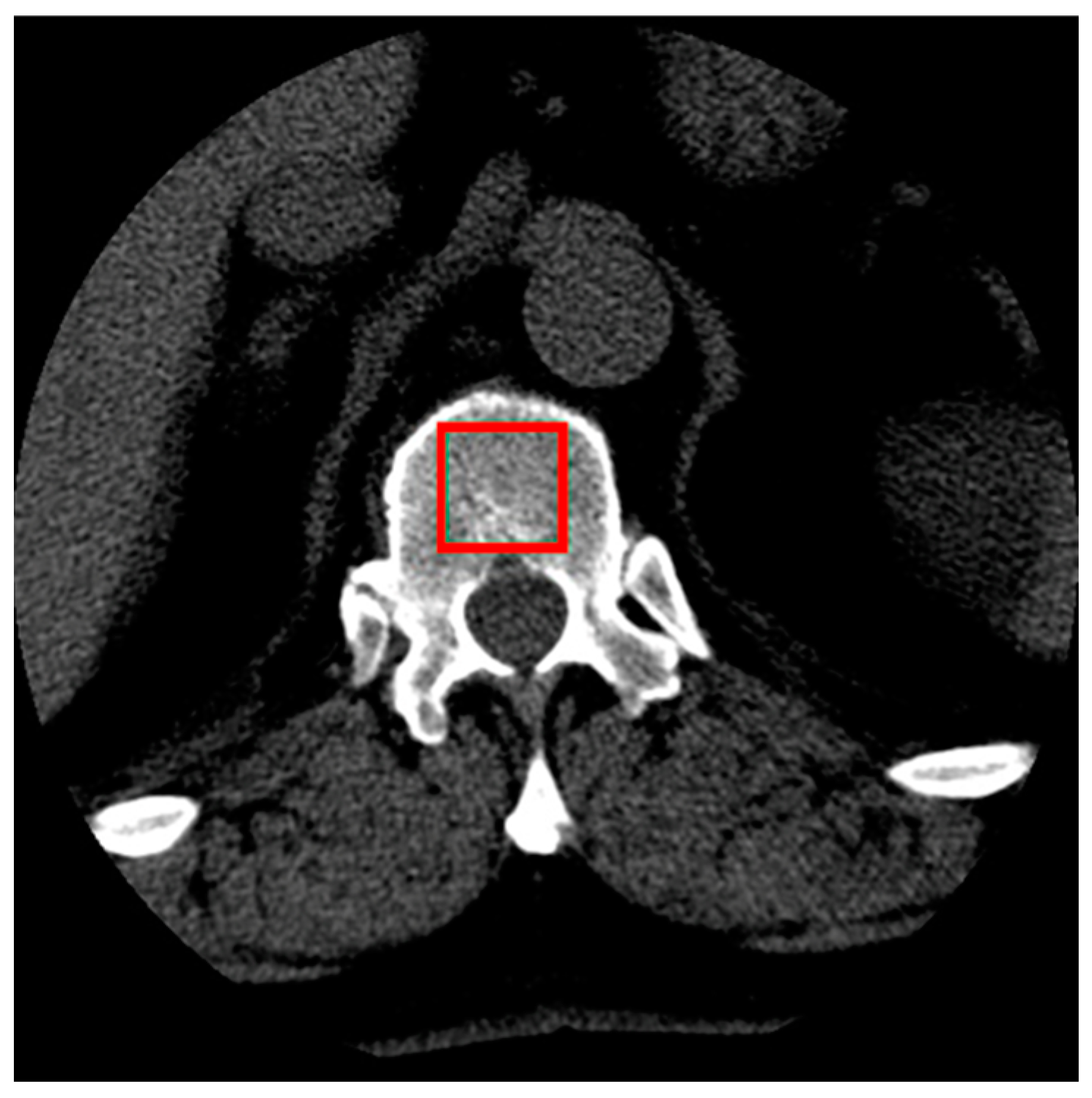
Sample cross-sections from the series of images were selected, showing the interior of the vertebra along with the cancellous bone. From each patient’s series of scans, four cross-sectional images of the L1 vertebra were selected. These images represented cross-sections closest to the midpoint of the vertebra’s height to ensure that the largest possible area of cancellous bone was visible (Figure 1). From each selected cross-sectional image, a single sample of the examined tissue image was obtained.

The size of the selected samples was chosen to maximize the use of the texture area containing potential information from the cross-sectional image of the vertebra. As a result, four hundred samples, each measuring 50 × 50 pixels, were obtained. Example images of tissue from healthy patients and patients with osteoporosis are shown below (Figure 2).

One of the commonly used actions during image preparation for further classification is the histogram normalization process. In previous studies conducted by the author, it was shown that this operation leads to a decrease in classification accuracy, ranging from 4% for the TPR coefficient to 14% for ACC [32].

The first stage of this study involved performing a texture analysis of the images using the MaZda program (version 4.6) [33]. This program enables the analysis of grayscale images and the determination of numerical values for various image features. The set of features was derived based on the following parameters: histogram (9 features including histogram mean, histogram variance, histogram skewness, histogram kurtosis, and percentiles at 1%, 10%, 50%, 90%, and 99%), gradient (5 features such as absolute gradient mean, absolute gradient variance, absolute gradient skewness, absolute gradient kurtosis, and the percentage of pixels with a nonzero gradient), run length matrix (5 features across 4 directions: run length nonuniformity, gray level nonuniformity, long run emphasis, short run emphasis, and the fraction of the image in runs), co-occurrence matrix (11 features across 4 directions and 5 inter-pixel distances: angular second moment, contrast, correlation, sum of squares, inverse difference moment, sum average, sum variance, sum entropy, entropy, difference variance, and difference entropy), autoregressive model (5 features: parameters Θ1, Θ2, Θ3, Θ4, and standard deviation), and Haar wavelet (24 features: wavelet energy calculated at 6 scales across 4 frequency bands LL, LH, HL, and HH) [33].

For each sample, 290 features were obtained. Features with constant values for each sample were eliminated. After reduction, 267 features remained. These were ranked by importance, from the most important to the least important. Figure 3 shows visualizations of the feature value distribution for the most important and least important features.

3. Results

The classification performance was evaluated using different numbers of features. A total of 267, 200, 150, 100, 50, 20, and 10 features were used to build the classifiers, respectively. Five learning methods were used: Naive Bayes (NBC), Multilayer Perceptron (MP), Hoeffding Tree (HT), K-Nearest Neighbors (1-NN), and Random Forest (RF). A ten-fold cross-validation was used for the classification process of each method. To evaluate the accuracy of the classifiers, the following metrics were used:

• Overall classification accuracy (ACC) measures the percentage of all cases that were correctly classified;
• True positive rate (TPR) measures the percentage of true positive cases that were correctly identified by the model;
• True negative rate (TNR) measures the percentage of true negative cases that were correctly identified by the model;
• Positive predictive value (PPV) measures the percentage of positive predicted examples that were actually positive;
• Negative predictive value (NPV) measures the percentage of negative predicted examples that were actually negative;
• A generalized version of the Pearson correlation coefficient evaluates the agreement between the model predictions and the actual classes (MCC);
• F1-score combines precision and sensitivity into one metric, taking into account the balance between these two parameters.

The classification results allow us to assess the effectiveness of each classifier depending on the number of features used. The obtained classification results are presented below. The best results for each method are marked in gray in the table.

Analyzing the data presented in

Table 1. Naive Bayes classification results.

Number of Features	ACC	TPR	TNR	PPV	NPV	MCC	F1 Score
267	83.00	76.50	89.50	76.50	89.50	66.60	81.80
200	87.00	84.50	89.50	84.50	89.50	74.10	86.64
150	87.25	85.50	89.00	85.50	89.00	74.50	87.02
100	87.25	86.00	88.50	86.00	88.50	74.50	87.09
50	88.50	87.00	90.00	87.00	90.00	77.00	88.33
20	88.25	86.50	90.00	86.50	90.00	76.50	88.02
10	88.25	86.50	90.00	86.50	90.00	76.50	88.02

, a clear influence from the number of features on the performance of various metrics is observed. A larger number of features, such as 267, leads to lower values for most metrics compared to scenarios where the number of features is reduced. Reducing the number of features to 50, and even to 20 or 10, results in a significant improvement across most metrics, although some indicators exhibit slight declines with a very small number of features. Positive predictive values (PPVs) and negative predictive values (NPVs) also show higher results with fewer features. The maximum values of 87.00% for PPVs and 90.00% for NPVs are achieved with 50 features. Further reductions to 20 or 10 features result in slight declines, yet these values remain high. Notably, the Matthews correlation coefficient (MCC) is highly sensitive to the number of features, with the lowest value (66.60%) observed at 267 features and the highest (77.00%) at 50 features, followed by a minor decrease to 76.50% for 20 and 10 features. The F1 score is the lowest at 267 features (81.80%), peaks at 88.33% with 50 features, and decreases marginally to 88.02% for 20 and 10 features. This indicates that 50 features represent an optimal balance between model accuracy and complexity.

The accuracy (ACC) reaches its lowest value at 267 features (83.00%), while the highest result (88.50%) is observed with 50 features, followed by a minimal decrease to 88.25% for 20 and 10 features. A similar trend is evident for sensitivity (TPR), which increases as the number of features decreases, peaking at 87.00% with 50 features and then slightly dropping to 86.50% for 20 and 10 features. Specificity (TNR), on the other hand, remains constant at 90.00% for 50, 20, and 10 features, which represents the highest value, compared to the lowest value (89.50%) at 267 features (Figure 4).

In conclusion, reducing the number of features to 50 emerges as the most optimal choice. Further reduction to 20 or 10 features can be advantageous in terms of computational efficiency, as it results in only a slight degradation of performance. Conversely, a very high number of features (267) significantly lowers model quality, particularly in terms of MCC and F1 score.

The multilayer perceptron method demonstrates a significant influence of the number of features on the performance of various classification parameters (

Table 2. Multilayer Perceptron classification results.

Number of Features	ACC	TPR	TNR	PPV	NPV	MCC	F1 Score
267	94.50	93.50	95.50	93.50	95.50	89.00	94.44
200	95.00	94.50	95.50	94.50	95.50	90.00	95.00
150	93.50	93.50	93.50	93.50	93.50	87.00	93.50
100	96.50	97.00	96.00	97.00	96.00	93.00	96.50
50	94.25	95.50	93.00	95.50	93.00	88.50	94.34
20	87.75	85.50	90.00	85.50	90.00	75.60	87.45
10	88.00	85.00	90.50	85.50	90.50	76.10	87.69

). Both an excessive and an insufficient number of features negatively affect the model’s effectiveness. The Matthews correlation coefficient (MCC), which measures the overall performance of the model, reaches its highest value (93.00%) with 100 features. With a higher number of features (200 and 267), MCC decreases slightly (90.00% and 89.00%, respectively). The lowest MCC values (75.60% and 76.10%) are observed with 20 and 10 features, indicating the negative impact of too few features on classification performance. A similar trend is observed for the positive predictive value (PPV) and negative predictive value (NPV), which reach their highest values (97.00% and 96.00%) with 100 features, confirming the optimality of this feature count for accurate classification of both classes. With fewer features, these values decrease slightly, reaching 85.50% for PPV and 90.50% for NPV with ten features. The F1 score also reaches its highest value (96.50%) with 100 features. Reducing the number of features below 50 results in a decline in the F1 score, which reaches its lowest value (87.45%) with 20 features. Although the F1 score with 267 features is 94.44%, it is lower than with 100 features.

The accuracy (ACC) of the model is highest with 100 features (96.50%), suggesting that this number of features provides the best balance between correctly classifying positive and negative cases. With 267 and 200 features, the accuracy decreases slightly to 94.50% and 95.00%, indicating a slight deterioration in performance due to feature redundancy. When the number of features is reduced below 50, accuracy drops significantly, reaching its lowest value (87.75%) with 20 features. A similar trend is observed for sensitivity (TPR), which reaches its highest value (97.00%) with 100 features, demonstrating the model’s best ability to correctly classify positive cases. Sensitivity gradually decreases as the number of features is reduced, reaching 85.00% with ten features, showing the loss of critical information necessary for effective classification. An excessive number of features, such as 267, also causes a decrease in sensitivity to 93.50%. Specificity (TNR) remains high (95.50%) with 200 and 267 features, indicating the model’s strong ability to detect negative cases with a higher number of features. However, as the number of features decreases, specificity drops to 93.00% with 50 features and 90.50% with 10 features (Figure 5).

The presented results suggest that 100 features is the optimal choice, providing the highest values for all evaluated metrics. Increasing the number of features to 200 or 267 still yields satisfactory results, but leads to a slight decrease in model efficiency. On the other hand, reducing the number of features too much (to 20 or 10) causes a clear deterioration in performance, indicating the loss of important information. Therefore, selecting the appropriate number of features, such as 100, appears to be the best compromise between model effectiveness and complexity.

For Hoeffding Tree classification, the Matthews correlation coefficient (MCC) achieves its highest value of 77.50% with 50 features. Reducing the number of features below 50 results in a decrease in MCC to 76.50% with 20 and 10 features, and with 267 features, the MCC drops to only 66.00%, indicating that an excess of features can lead to a degradation of the overall model quality. A similar trend is observed in the F1 score, which reaches its highest value of 88.57% with 50 features. With 20 and 10 features, the F1 score is 88.02%, reflecting only a minimal decrease in performance with fewer features. However, with 267 features, the F1 score is reduced to 81.59%. Similar relationships are evident in the predictive values for the positive class (PPV) and the negative class (NPV). The highest values of PPV (87.00%) and NPV (90.50%) are achieved with 50 features. With fewer features, these values slightly decrease, reaching 86.50% for PPV and 90.00% for NPV with 20 and 10 features. However, with 267 features, PPV and NPV are reduced to 76.50% and 89.00%, respectively, indicating a decline in prediction quality (

Table 3. Hoeffding Tree classification results.

Number of Features	ACC	TPR	TNR	PPV	NPV	MCC	F1 Score
267	82.75	76.50	89.00	76.50	89.00	66.00	81.59
200	86.50	84.00	89.00	84.00	89.00	73.10	86.14
150	87.00	85.50	88.50	85.50	88.50	74.00	86.78
100	87.25	86.00	88.50	86.00	88.50	74.50	87.09
50	88.75	87.00	90.50	87.00	90.50	77.50	88.57
20	88.25	86.50	90.00	86.50	90.00	76.50	88.02
10	88.25	86.50	90.00	86.50	90.00	76.50	88.02

).

The highest accuracy (ACC) is achieved with 50 features (88.75%), suggesting that this number of features provides the best balance between correctly classifying both positive and negative cases. Reducing the number of features below 50 results in only a minimal decrease in accuracy (88.25% with 20 and 10 features); however, with 267 features, the accuracy drops to 82.75%, indicating a negative impact of excessive features on the model’s performance. Sensitivity (TPR) increases as the number of features is reduced, reaching its highest value of 87.00% with 50 features. With 267 features, sensitivity drops to only 76.50%, showing that an excess of features reduces the model’s ability to correctly classify positive cases. Reducing the number of features below 50 results in a gradual decline in sensitivity, reaching 86.50% with 20 and 10 features. Specificity (TNR) remains high with 50 features (90.50%) and does not change significantly with further reduction in the number of features, reaching 90.00% with 20 and 10 features. In contrast, with 267 features, specificity is 89.00%, representing a slight decrease (Figure 6).

The optimal number of features, which provides the best results across most metrics, is 50 features. Reducing the number of features below 50 causes only a slight deterioration in performance, while an excess of features (267) leads to a decline in model effectiveness, particularly in terms of MCC, PPV, NPV, and F1 score.

The classification results obtained using the K-Nearest Neighbors (K-NN) method for K = 1, as presented in the table (

Table 4. K-Nearest Neighbors classification results.

Number of Features	ACC	TPR	TNR	PPV	NPV	MCC	F1 Score
267	93.25	95.00	91.50	95.00	91.50	86.60	93.18
200	94.25	96.50	92.00	96.50	96.50	88.60	94.55
150	94.75	96.50	93.00	96.50	93.00	89.60	94.59
100	96.50	98.50	94.50	98.50	94.50	93.10	96.12
50	96.75	97.50	96.00	97.50	96.00	93.50	96.23
20	81.50	82.50	80.50	82.50	80.50	63.00	81.77
10	85.25	85.50	85.00	85.50	85.00	70.50	85.30

) based on the number of features, highlight the differences in model performance in terms of various quality metrics. The Matthews correlation coefficient (MCC) reaches its highest value of 93.50% with 50 features, indicating the model’s best overall performance in this case. MCC gradually decreases as the number of features is reduced below 50, reaching 86.60% with 267 features and 63.00% with 20 features, suggesting a significant deterioration in model quality with fewer features. At 10 features, MCC increases to 70.50%, representing some improvement compared to the value observed with 20 features. Similarly, the F1 score also achieves its highest value of 96.23% with 50 features. The F1 score gradually declines as the number of features decreases, reaching 96.12% with 100 features, 94.59% with 150 features, and 94.55% with 200 features. At 20 features, the F1 score is 81.77%, and at 10 features, it increases to 85.30%, indicating a decrease in classification quality with too few features. The positive predictive value (PPV) and negative predictive value (NPV) both reach their highest values with 100 features, being 98.50% and 96.00%, respectively. These values gradually decrease as the number of features is reduced, reaching 97.50% for PPV and 96.00% for NPV with 50 features. At 20 features, PPV and NPV drop to 82.50% and 80.50%, respectively, suggesting a decline in prediction quality with too few features. At 10 features, PPV is 85.50% and NPV is 85.00%, showing a slight improvement compared to the values observed with 20 features.

The highest accuracy (ACC) of 96.75% was achieved with 50 features. Accuracy slightly decreases as the number of features is reduced below 50, reaching 96.50% with 100 features and 94.75% with 150 features. However, with a further reduction to 20 features, accuracy sharply declines to 81.50%, and with 10 features, it increases to 85.25%, suggesting a significant loss in classification quality when too few features are used. The sensitivity (TPR) reaches its highest value of 98.50% with 100 features. As the number of features decreases below 100, sensitivity gradually decreases to 97.50% with 50 features, 96.50% with 150 features, and 95.00% with 267 features. Sensitivity significantly drops to 82.50% with 20 features, and then increases slightly to 85.50% with 10 features, which may indicate a better model fit to the data with this number of features. The specificity (TNR) remains high with 50 features (96.00%). With 100 features, specificity is 94.50%, and with 150 features, it is 93.00%. However, with 20 features, specificity drops to 80.50%, indicating a loss in the model’s ability to correctly classify negative cases with too few features. With 10 features, specificity increases to 85.00%, representing an improvement compared to the value obtained with 20 features (Figure 7).

The optimal number of features that provides the best classification results using the K-NN method is 50 features. Reducing the number of features below 50 leads to a gradual decline in performance, particularly in terms of MCC, PPV, NPV, F1, and TPR. An excess of features (267 features) results in a slight deterioration in performance, indicating that the K-NN model achieves better results with a smaller number of relevant features.

The classification results using the Random Forest method (

Table 5. Random Forest classification results.

Number of Features	ACC	TPR	TNR	PPV	NPV	MCC	F1 Score
267	90.25	90.00	95.00	90.00	90.50	80.50	93.18
200	90.75	91.00	90.50	91.00	90.50	81.50	94.55
150	91.25	91.00	91.50	91.00	91.50	82.50	94.59
100	90.75	90.00	91.50	90.00	91.50	81.50	96.12
50	91.75	92.00	91.50	92.00	91.50	83.50	96.23
20	87.00	86.00	88.00	86.00	88.00	74.00	81.77
10	86.50	85.50	87.50	85.50	87.50	73.00	85.30

), depending on the number of features, indicate significant changes in model performance. The Matthews correlation coefficient (MCC) reaches its highest value of 83.50% with 50 features, suggesting the best overall quality of the model. A decline in MCC is observed with fewer features, reaching 73.00% with ten features. The highest F1 score (96.23%) was achieved with 50 features, indicating that the model best balances both sensitivity and specificity with this number of features. With ten features, the F1 score drops to 85.30%, representing a noticeable deterioration compared to the results obtained with a larger number of features. The highest predictive values for the positive class (PPV) and the negative class (NPV) were achieved with 50 features, being 92.00% and 91.50%, respectively. These values gradually decrease as the number of features is reduced, reaching 90.00% PPV and 91.50% NPV with 100 features. With 10 features, PPV is 85.50% and NPV is 87.50%, representing an improvement compared to 20 features, but still lower than with a larger number of features.

The highest accuracy (ACC) was achieved with 50 features, 91.75%. When the number of features was reduced below 50, the accuracy slightly decreased, reaching 90.75% with 100 features, 91.25% with 150 features, and 90.75% with 200 features. With 267 features, the accuracy was 90.25%. On the other hand, with 20 features, the accuracy dropped to 87.00%, and with 10 features, it was 86.50%, indicating a significant loss of classification quality with too few features. Sensitivity (TPR) reached its highest value of 92.00% with 50 features, and gradually decreased with fewer features, reaching 90.00% with 100 features, 91.00% with 150 features, and 91.00% with 200 features. With 267 features, sensitivity was 90.00%, and with 10 features, it was 85.50%, suggesting that fewer features impact the model’s ability to detect positive cases. Specificity (TNR) remained high at 50 features (91.50%) and then slightly decreased to 90.50% with 100 features, 91.50% with 150 features, and 90.50% with 200 features. The highest specificity (95.00%) was obtained with 267 features, while the lowest (87.50%) was obtained with 10 features, indicating a reduced ability of the model to classify negative cases with too few features (Figure 8).

The optimal number of features for the Random Forest method that provides the best classification results is 50 features. Reducing the number of features below 50 leads to a gradual decline in model performance, particularly in terms of MCC, PPV, NPV, F1 score, and TPR. An excess of features (267 features) slightly improves some metrics, but with 10 features, the model achieves significantly worse results, indicating a substantial deterioration in classification quality.

The analysis of the classification results for different classifiers, depending on the number of features, reveals significant variations in the effectiveness of the respective methods (

Table 6. Summary of results by number of features for classifiers: Naïve Bayes(NB), Multilayer Perceptron (MLP), Hoeffding Tree (HT), K-Nearest Neighbors (KNN), and Random Forest (RF).

Number of Features	Classifier	ACC	TPR	TNR	PPV	NPV	MCC	F1 Score
267	NB	83.00	76.50	89.50	76.50	89.50	66.60	81.80
	MLP	94.50	93.50	95.50	93.50	95.50	89.00	94.44
	HT	82.75	76.50	89.00	76.50	89.00	66.00	81.59
	KNN	93.25	95.00	91.50	95.00	91.50	86.60	93.37
	RF	90.25	90.00	95.00	90.00	90.50	80.50	90.25
200	NB	87.00	84.50	89.50	84.50	89.50	74.10	86.64
	MLP	95.00	94.50	95.50	94.50	95.50	90.00	95.00
	HT	86.50	84.00	89.00	84.00	89.00	73.10	86.14
	KNN	94.25	96.50	92.00	96.50	96.50	88.60	94.35
	RF	90.75	91.00	90.50	91.00	90.50	81.50	90.75
150	NB	87.25	85.50	89.00	85.50	89.00	74.50	87.02
	MLP	93.50	93.50	93.50	93.50	93.50	87.00	93.50
	HT	87.00	85.50	88.50	85.50	88.50	74.00	86.78
	KNN	94.75	96.50	93.00	96.50	93.00	89.60	94.82
	RF	91.25	91.00	91.50	91.00	91.50	82.50	91.25
100	NB	87.25	86.00	88.50	86.00	88.50	74.50	87.09
	MLP	96.50	97.00	96.00	97.00	96.00	93.00	96.50
	HT	87.25	86.00	88.50	86.00	88.50	74.50	87.09
	KNN	96.50	98.50	94.50	98.50	94.50	93.10	96.56
	RF	90.75	90.00	91.50	90.00	91.50	81.50	90.69
50	NB	88.50	87.00	90.00	87.00	90.00	77.00	88.33
	MLP	94.25	95.50	93.00	95.50	93.00	88.50	94.34
	HT	88.75	87.00	90.50	87.00	90.50	77.50	88.57
	KNN	96.75	97.50	96.00	97.50	96.00	93.50	96.79
	RF	91.75	92.00	91.50	92.00	91.50	83.50	91.75
20	NB	88.25	86.50	90.00	86.50	90.00	76.50	88.02
	MLP	87.75	85.50	90.00	85.50	90.00	75.60	87.45
	HT	88.25	86.50	90.00	86.50	90.00	76.50	88.02
	KNN	81.50	82.50	80.50	82.50	80.50	63.00	81.69
	RF	87.00	86.00	88.00	86.00	88.00	74.00	86.89
10	NB	88.25	86.50	90.00	86.50	90.00	76.50	88.02
	MLP	88.00	85.00	90.50	85.50	90.50	76.10	87.69
	HT	88.25	86.50	90.00	86.50	90.00	76.50	88.02
	KNN	85.25	85.50	85.00	85.50	85.00	70.50	85.30
	RF	86.50	85.50	87.50	85.50	87.50	73.00	86.34

). The highest performance was achieved by the K-Nearest Neighbors (K = 1) and Multilayer Perceptron classifiers. KNN demonstrated the best results with 50 features, attaining a highest F1 score of 96.79% and accuracy (ACC) of 96.75%. This model also exhibited exceptionally high positive predictive value (PPV) and true positive rate (TPR), both at 97.50%, indicating excellent balance between positive and negative class predictions. MLP achieved its optimal performance with 100 features, reaching an accuracy and F1 score of 96.50%. Furthermore, the model’s sensitivity (TPR) was 97.00%, while specificity (TNR) stood at 96.00%, underscoring its high classification efficacy. Below are the confusion matrices for the best models (Figure 9).

Among the weakest classifiers were Hoeffding Tree and Naïve Bayes. HT demonstrated consistently low metric values across most scenarios, particularly with 267 features, where its accuracy was 82.75% and F1 score was only 81.59%. Similarly, NB recorded its poorest performance with 267 features, achieving an accuracy of 83.00% and a MCC of 66.60%. Although both models improved their results with fewer features, they were outperformed by other methods. KNN, despite its excellent performance with 50 features, experienced a significant decline in quality with 10 features, where accuracy dropped to 85.25% and the F1 score dropped to 85.30%. This suggests that KNN requires an adequate number of features to maintain effective classification.

In summary, the optimal number of features for most classifiers ranges from 50 to 100, enabling the highest classification outcomes. An excessive number of features (267) or an insufficient number (10–20) leads to substantial degradation in classification quality. Among the analyzed classifiers, KNN and MLP consistently demonstrated superior performance, whereas HT and NB were the least effective.

4. Discussion

In order to analyze the effectiveness of the classifications using different numbers of texture features of spongy tissue images, the obtained results were compared with the results obtained by the author in previous studies. The results presented in [31,32] are based on the same set of images, but different approaches to processing textural features were used. Comparing the results allows for the assessment of the impact of the applied methods on the efficiency of classification, as well as for indicating the potential advantages or limitations of the analyzed method.

In the study by [31], after the determination of the texture features of the tissue images, a selection process was performed. Data reduction consisted of feature selection, the aim of which was to reduce the initial set of 290 features to a smaller subset containing only those features that were most important from the point of view of the classification criterion. After data cleaning, which aimed to remove features with constant values, duplicates and strongly correlated, and the number of features was reduced to 18 for the reconstruction of soft tissues. The selection of features was performed using nine methods divided into three groups: filtering methods (Fisher method and analysis of variance and Relief method), wrapper methods (Sequential Forward Selection, Sequential Backward Selection, and Recursive Feature Elimination with the LogisticRegression estimator), and embedded methods (SelectFromModel with different estimators, such as Logistic Regression, AdaBoost, and LightGBM).

In the case of soft tissue reconstruction, the best models achieved a highest classification accuracy of 95% with a validation accuracy of 96%. Models that used different feature selection methods achieved identical TPR (sensitivity) and TNR (specificity) values of 95% each. The model based on NuSVM with an ANOVA feature selection method using 17 features achieved high accuracy and was one of the best. The model that used SVM with the RELIEF feature selection method and 18 features and the model based on NuSVM with the same RELIEF method also achieved very good results, achieving 95% in TPR and TNR. Models that used SVM and NuSVM with the RFE feature selection method and 18 features also achieved identical results (95% TPR and TNR).

The aim of the research presented in the article by [32] was to determine the effect of normalizing CT spine images on the accuracy of automatic recognition of defects in the spongy tissue structure of the vertebrae in the thoracolumbar section. Feature descriptors were based on a gray level histogram, gradient matrix, RL matrix, event matrix, autoregressive model, and wavelet transformation. Six feature selection methods were used: Fisher coefficient, minimization of the probability of classification error with the accumulated correlation coefficient, mutual information, Spearman correlation, heuristic identification of confounding variables, and linear stepwise regression. The selection results were used to build six popular classifiers: Linear and Quadratic Discriminant Analysis, Naive Bayes Classifier, Decision Tree, K-Nearest Neighbors, and Random Forests. For the applied set of textural features and the selection and classification methods, image normalization significantly worsened the accuracy of the automatic recognition of osteoporosis based on CT spine images. The most accurate results obtained with quadratic discriminant analysis and K-nearest neighbors (K = 5) classification were ACC = 95%.

Comparing the results presented in

Table 7. Comparison of classification results in relation to the author’s previous research.

No. in Ref.	Number of Features	Feature Selection Method	Classification Method	ACC (%)	TPR (%)	TNR (%)
Current research	50	-	KNN	96.75	97.50	96.00
Current research	100	-	MLP	96.50	97.00	96.00
[31]	17	ANOVA	NuSVM	95.00	95.00	95.00
[31]	18	RELIEF	SVM	95.00	95.00	95.00
[31]	18	RELIEF	NuSVM	95.00	95.00	95.00
[31]	18	RFE	SVM	95.00	95.00	95.00
[31]	18	RFE	NuSVM	95.00	95.00	95.00
[32]	6	POE + ACC	5-NN	90.00	85.71	95.36
[32]	6	LSR	QDA	90.00	87.50	92.50

, it is possible to see differences in the performance of different classification models, both in terms of accuracy (ACC), sensitivity (TPR), and specificity (TNR). The best results were obtained in the two experiments of the current study, where KNN and MLP models with different numbers of features were used. The KNN model with 50 features achieved an accuracy of 96.75%, which is the highest result in the table. In addition, a high sensitivity of 97.50% and a specificity of 96.00% were obtained. In a very similar way, the MLP model with 100 features achieved an ACC of 96.50%, TPR of 97.00%, and TNR of 96.00%. These results indicate that these models are characterized by excellent performance in identifying both positive and negative cases, with high accuracy and balanced sensitivity and specificity. Compared to these results, the study by [31] shows that using different feature selection methods (such as ANOVA, RELIEF or RFE) in combination with SVM and NuSVM classifiers gave slightly worse results. In all these cases, the accuracy was 95%, and the sensitivity and specificity were 95%. Although these results are robust and show a balance between detecting positive and negative cases, they are still lower than those achieved by KNN and MLP. On the other hand, in the study by [32], where fewer features were used (six features), the 5-NN and QDA models achieved an accuracy of 90%, which is the lowest result in the table. The 5-NN model also achieved a relatively low sensitivity of 85.71%, despite a very high specificity of 95.36%. The QDA model had a higher sensitivity (87.50%), but a lower specificity (92.50%). Although both models achieved equal accuracy, the differences in sensitivity and specificity indicate some trade-offs that had to be accepted as a result of using fewer features.

The table below (

Table 8. Summary of the results of similar bone texture analysis tests [31].

No. in Ref.	Texture Features	ROI Segmentation	Dataset	Classifier	TPR	TNR	PPV	NPV	ACC	F1-Score
current research	Histogram, Gradient, Run length matrix, Cooccurrence, Autoregressive, Haar wavelet	Manual	50 cases and 50 controls	KNN	97.50	96.00	97.50	96.00	96.75	96.50
current research	Histogram, Gradient, Run length matrix, Cooccurrence, Autoregressive, Haar wavelet	Manual	50 cases and 50 controls	MLP	97.00	96.00	97.00	96.00	96.50	96.00
[34]	1D projection modeled as fractional Brownian motion	Calcaneal (Manual)	-	SVM	96.9	97.6	-	-	94.5	94.3
[35]	Fractional Brownian model and Rao geodesic distance	Calcaneal	348 cases and 348 controls	KNN	97.8	95.4	-	-	96.6	96.5
[36]	Histogram and GLCM and PCA analysis	Calcaneal (Manual)	87 cases and 87 controls	SVM	97.7	95.4	95.5	97.7	96.6	96.6
[37]	Anisotropic discrete dual-tree wavelet transform	Calcaneal (Manual)	87 cases and 87 controls	SVM	-	93.1	92.9	91.0	91.9	91.9
[38]	Wavelet decomposition and parametric circular models	Calcaneal (Manual)	87 cases and 87 controls	SVM	100	92.5	91.9	100	95.9	95.8

) compares the obtained research results with the results of other authors who conducted similar studies and achieved high effectiveness using their methods. The quality of the models built should be assessed as high. Considering the total classification accuracy (ACC), it can be seen that the obtained result is the highest and that most of the results presented in the table are much lower. Analyzing the data, it can be stated that the presented method stands out from similar studies and shows high diagnostic potential.

The results presented in this work demonstrate the diagnostic potential of the proposed methods, which could serve as the basis for developing a screening procedure routinely performed for individuals in a specific age group at risk of bone tissue loss. A solution that could positively impact osteoporosis diagnostics is the creation of an additional diagnostic module for the software used in medical facilities, enabling automatic analysis of bone tissue texture during examinations conducted for other diagnostic purposes. If such tissue image analysis were possible during CT scans, for example, in individuals involved in accidents where the examination is aimed at detecting potential injuries, it would significantly broaden the group of individuals tested and allow for the detection of changes in bone tissue in patients who would likely not be referred for specialized tests for bone mass loss. This type of solution would not incur additional costs, as it would be based on images used for diagnosing other conditions.

5. Conclusions

In summary, based on the conducted research and analysis of their results, it can be concluded that the number of features used in classification is a key factor that affects the quality and efficiency of the model. Classifiers based on a larger number of features (50 and 100 features) achieved better results in terms of accuracy (ACC), sensitivity (TPR), and specificity (TNR). Especially, KNN with 50 features and MLP with 100 features achieved very high accuracy at levels of 96.75% and 96.50%, which suggests that a larger number of features allows for better capturing important information in the data. These models were able to achieve high sensitivity (97.50% and 97.00%) and specificity (96.00%), which indicates their ability to effectively classify both positive and negative cases. Therefore, in applications requiring high precision, a larger number of features can improve the classification quality.

In the case of models using only six features (as in [32]), the results were noticeably worse, with an accuracy of 90%, which is the lowest result in the studies. Although the 5-NN model achieved high specificity (95.36%), its sensitivity (85.71%) was much lower. The QDA model had higher sensitivity (87.50%), but lower specificity (92.50%). These differences indicate that a smaller number of features limits the model’s ability to capture the full structure of the data, which affects its performance, especially in the case of detecting positive cases. The use of different feature selection methods, such as RELIEF, RFE, or ANOVA, in combination with different classifiers (SVM, NuSVM), leads to stable but slightly lower results than those obtained by models with more features. Although this approach provides a balance between detecting positive and negative cases, its results do not reach the level of those obtained by more advanced classification models with more features.

Finally, the results suggest that selecting the appropriate number of features is crucial to achieve a high-quality classification model. A larger number of features allows us to better capture the complexity of the data, which translates into higher classification results, while limiting the number of features may lead to a decrease in performance, especially in cases where important information is contained in a larger number of features. Therefore, future studies should focus on further optimizing the number of features and feature selection methods to achieve the best results in the context of osteoporosis diagnosis based on CT scans of spongy tissue.