Multi-Objective Optimisation of Welding Parameters for AZ91D/AA6082 Rotary Friction Welded Joints

Abstract

Recently, rotary friction welding has been used to join magnesium alloys. FRW uses friction heat to bond magnesium alloys with aluminium alloys. Combining these light alloys can provide many promising applications in the industry. The welding parameters such as friction and upsetting force, rotational speed, and welding time play a significant role in determining the joint strength. The paper presents a new approach to multi-objective optimisation of friction welding process parameters for AZ91D/AA6082 alloy joints. Multi-objective optimisation is based on artificial neural networks and genetic algorithms as non-conventional AI techniques. The methods were used to determine the following optimal welding process parameters: friction force, upsetting force and friction time for simultaneously maximised tensile strength and minimised metal loss (shortening) during welding. The ultimate tensile strength and metal loss of the friction welding joints were studied numerically and experimentally. Moreover, the influence of welding parameters on the ultimate tensile strength and shortening of friction joints was also studied. A genetic algorithm successfully found a set of welding parameters for which the joint strength increases from 24 to 81 MPA and the joint shortening decreases from 8.25 to 0.23 mm. The results show that a low friction force and upsetting force give a high value of tensile strength and the lowest shortening of the bimetal joints.

1. Introduction

Recently, much attention has been focused on magnesium and aluminium alloys in many industrial sectors because of their unique properties. For their practical applications, joining technologies should also be developed in addition to considering issues such as alloy design, microstructure control, plastic forming, casting, and surface treatment [1]. Combining aluminium alloys with magnesium alloys contributes to reducing the weight of components and increasing production efficiency by replacing aluminium alloys with magnesium alloys wherever possible. Joining the mentioned metals is very difficult using conventional welding methods [2]. During standard joining, due to the melting of materials and a large amount of heat supplied, significant grain growth occurs in the heat-affected zone (HAZ), and many brittle intermetallic metal compounds (IMCs) are formed [3]. The aluminium–magnesium equilibrium system has partial solubility of magnesium and aluminium. However, in the range of several percent by weight and the remaining compositions, the IMCs are made [4,5]. The magnesium alloy was efficiently joined with the aluminium alloy by laser [6,7] and diffusion welding methods [8,9]. Various Mg/Al joints are made primarily by friction stir welding (FSW) to take advantage of the lower ability to form an intermetallic phase in the case of solid-state welding [10,11,12]. Authors in the following papers [10,13,14] observed the presence of precipitates of the intermetallic phase, which caused a substantial increase in hardness at the weld zone. The defect-free joints were observed for various rotational speeds in the study [15]. Moreover, no intermetallic phases or cracks were found in the joint area. The maximum value of 132 MPa tensile strength and extremely low elongation of 2% was achieved for a tool rotation speed of 1000 rpm in reference [16]. The literature results indicate the possibility of producing sound Mg/Al welded joints with different mechanical properties using solid-state friction welding methods [17,18].

Recently, a relatively common solid-state welding method is rotary friction welding (FRW) [19]. Friction welding of metals can be performed using an inertia friction welding (IFW) or direct-drive rotational friction welding (DD-FRW) process. In the IFW, the rotating part is connected to a flywheel, and energy is supplied to the joint through the loss of kinetic rotational energy. The DD-FRW method directly converts mechanical energy into thermal energy on mutually rubbing surfaces in the contact area [20]. The friction welding process can be divided into two periods: friction and upsetting. The key parameters of the FRW process are friction time (FT), friction force (FF), upsetting force (UF) and rotational speed (RS). The parameters determine the temperature in the contact area and the temperature gradient in the weld zone. Friction time is necessary to heat the elements to the required temperature. The key process parameter during the upsetting period is the upsetting force (UF). The UF parameter is applied to heated metals. The upsetting force brings the crystals of the rubbing surfaces closer to the distance of the spatial mesh [21]. Moreover, the upsetting parameter facilitates the diffusion process and leads to the consolidation of the joint. The optimisation of welding parameters is necessary for the proper course of thermal phenomena and its effects on the mechanical properties and microstructure of the joint [20].

Many works have presented the optimisation of welding parameters for dissimilar metals using statistical methods, neural networks, response surface methods, factorial design, genetic algorithms, or hybrid artificial intelligence methods. A factorial design for selecting the process parameters and predicting the bead width, height and penetration in the joint was investigated [22]. The optimal weld pool geometry in the tungsten insert gas (TIG) welding of the stainless steel was studied [23]. The authors [24] intensively explored the effect of process parameters on the weld pool geometry using the Taguchi method. A statistical response surface method for optimising welding parameters was developed [25,26]. Multi-regression methods and neural network models to predict optimal weld parameters were also analysed in [27,28,29]. The neural networks have been used to identify the welding parameters in real-time [30]. ANNs successfully predicted the desired weld beam geometry in gas metal arc welding. The optimal process parameters like feed rate, welding voltage and weld speed have been found to predict the beam height and depth of penetration of the weld beam [31]. Simulated annealing (SA) was also applied as an intelligent method for optimising welding parameters and weld pool in the TIG welding process [32]. The neural networks and genetic algorithm as the hybrid intelligent method were also studied to search optimal process parameters [33,34,35]. The evolutionary algorithms (EAs), particle swarm (PSO) and SA algorithms have been used to determine welding parameters to maximise tensile strength and minimise metal loss in friction welding steel [36]. A multi-objective optimisation for maximising the tensile strength and minimising the flash diameter and the HAZ width for the ductile iron with low-carbon steel joints was carried out in the study [37]. A genetic algorithm modeling temperature distribution during heating and cooling AZ31B magnesium alloys with 7075 aluminium alloy friction welded joints was investigated [38].

Rotary friction welding is a suitable welding method for joining light (Mg and Al) alloys [39,40]. In addition, FRW between dissimilar materials has recently received much attention [41]. However, more research is needed to optimise dissimilar FRW between Mg and Al alloys with relatively high strength using the conventional friction welding method [42,43,44,45]. In addition, it is difficult to fully understand the effects of basic processing parameters such as friction force, upsetting force and friction time on the dissimilar FRW between magnesium and aluminium alloys.

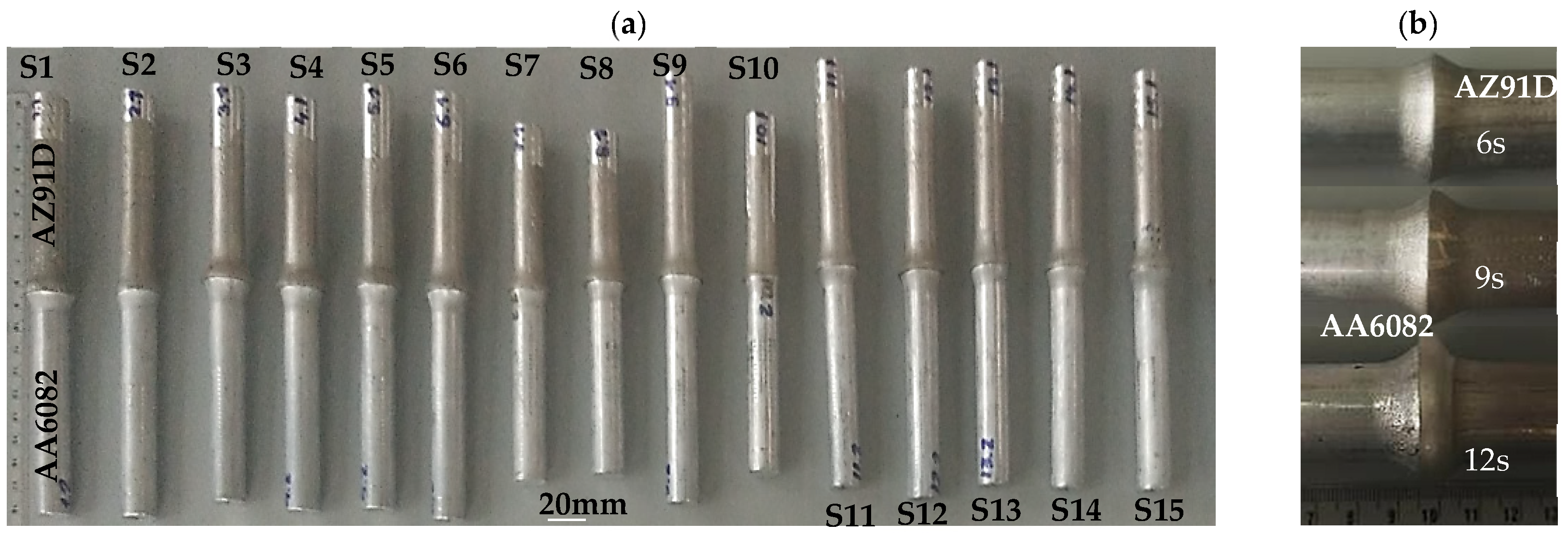
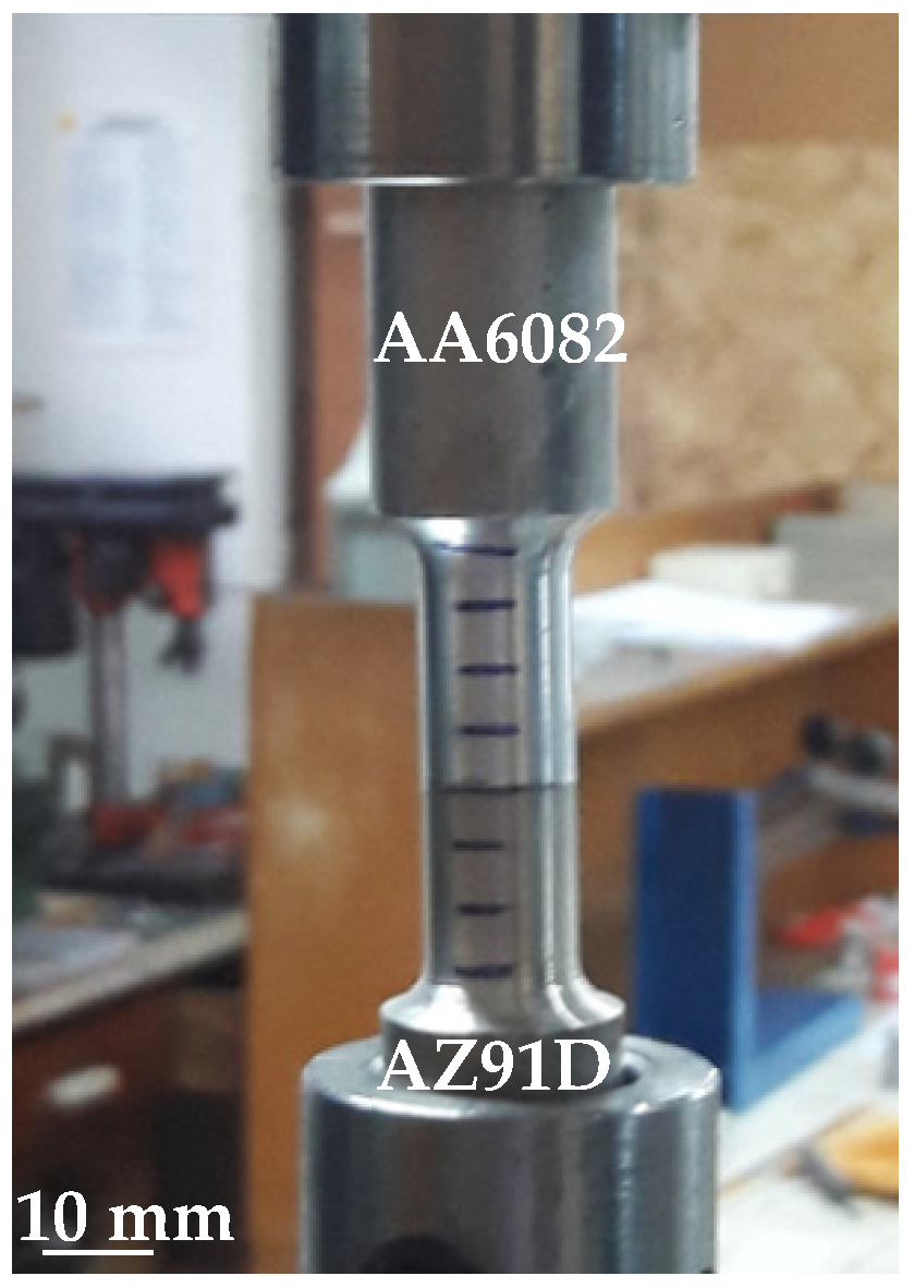
In this study, the previous joining of AZ91D with 6xxx series alloy bars by the direct-drive friction welding method was conducted. Then, the influences of the welding parameters on tensile properties and metal loss of the joints were experimentally and numerically investigated.

2. Materials and Methods

2.1. Materials

The rotary friction welding was carried out on AZ91D magnesium alloy and 6082T6 aluminium alloy bars of 20 mm in diameter and 100 mm in length. Bars were obtained by the extrusion process. The chemical composition and mechanical properties of the base metals are shown in

Table 1. Alloying elements (wt.%) of parent materials.

Material	Chemical Composition
	Mg	Al	Zn	Cu	Si	Mn
AZ91D	Rest	8.5–9.5	0.45–0.9	0.02	0.08	0.17–0.4
AA6082	0.60–1.20	Rest	0.20	0.10	0.70–1.30	0.40–1.0

and

Table 2. The mechanical properties of base materials.

Material	Mechanical Properties
	Tensile Strength	Yield Strength	Elongation A5	Hardness
	(MPa)	(MPa)	(%)	(HB)
AZ91D	280	160	7	49
AA6082	310	260	8	95

.

Before welding, the surfaces were prepared on the abrasive cut-off machine. After that, all contacting surfaces of samples were polished using grit silicon carbide papers to reduce the effect of oxide films and surface roughness. The specimens were cleaned in acetone to remove dirt and grease.

2.2. Sample Preparation

Figure 1a shows the friction welding process on a continuous drive friction machine (ZT4-13 type). The aluminium alloy bar is rotated with the spindle during welding, and the magnesium bar is moved axially under the axial pressure. A detailed diagram of the welding process cycle is shown in Figure 1b. The samples are pressed under an axial force after reaching the desired rotational speed (RS). The heated contact surfaces rub against each other, and the metal slowly squeezes out as a flash (see Figure 1a). The rotation of the sample stops, and upsetting force (UF) is applied to consolidate the welding joint, as shown in Figure 1a. A set of reducers and compressed air valves performs the welding machine’s work cycle. The air pressure during the friction and welding phases was set according to the graph shown in Figure 1c.

The process parameters used in the welding process are shown in

Table 3. The welding parameters.

No.	Friction Force (kN)	Friction Time (s)	Upsetting Force (kN)
S1	35	6	40
S2	45	6	40
S3	35	12	40
S4	45	12	40
S5	35	6	50
S6	45	6	50
S7	35	12	50
S8	45	12	50
S9	35	9	45
S10	45	9	45
S11	40	6	45
S12	40	12	45
S13	40	9	40
S14	40	9	50
S15	40	9	45

. The choice of parameters for welding was based on the previous reports [43,44,45,46]. In the experiment, the rotational speed (RS) and upsetting time were constant and equal to 1450 rpm and 6 s, respectively.

2.3. Macrographs

The joining of the magnesium to aluminium alloy was conducted successively using a conventional friction welding process. Macrographs of the welded samples with various welding conditions (see Table 3) are shown in Figure 2.

Before and after FRW, the length of the samples was measured to calculate the amount of material loss (shortening) during welding. Material loss (ML) is the difference between the total lengths (TLs) of both materials and the length of the friction weld (WL) after welding. The flashes in Figure 2 were symmetrically formed around the weld interface on magnesium and aluminium alloy sides. Flash formation increased with metal loss. During welding, the accumulated friction heat is enough to soften the base metal. The heated metal reaches a plastic state and is removed outwards due to the action of an axial force. Also, plastic deformation increased with increasing friction welding time, as shown in Figure 2b.

2.4. Testing

A tensile test was conducted on universal testing Instron, a servo-controlled machine (100 kN) at a constant movement rate of 1 mm/min (Figure 3). Room temperature tensile tests were carried out as per the ASTM:E8/E8M-13a standard specimen pattern [19].

Three specimens were tested for each group of welding parameters. From each Mg/Al joint, the average of three tests was recorded.

3. The Basic Experimental Results

The basic experimental results of the tensile strength and shortening measurements of the materials after the tensile test are presented in

Table 4. Experimental results of tensile strength and metal loss.

No.	Inputs			Outputs
	FF (kN)	UF (kN)	FT (s)	TS (MPa)	ML (mm)
1	35	40	6	25	10.82
2	35	40	6	26	10.83
3	35	40	6	24	10.81
4	45	40	6	30	6.76
5	45	40	6	31	6.77
6	45	40	6	29	6.75
7	35	50	6	80	8.01
8	35	50	6	81	8.02
9	35	50	6	79	8.00
10	45	50	6	64	4.13
11	45	50	6	65	4.15
12	45	50	6	63	4.12
13	35	40	12	72	11.4
14	35	40	12	73	11.6
15	35	40	12	71	11.2
16	45	40	12	64	9.78
17	45	40	12	65	9.80
18	45	40	12	63	9.72
19	35	50	12	56	40.6
20	35	50	12	57	40.8
21	35	50	12	55	40.4
22	45	50	12	59	40.33
23	45	50	12	60	40.36
24	45	50	12	58	40.30
25	35	45	9	65	6.80
26	35	45	9	66	7.00
27	35	45	9	64	6.60
28	45	45	9	45	34.95
29	45	45	9	46	35.00
30	45	45	9	44	34.85
31	40	40	9	61	6.00
32	40	40	9	62	6.50
33	40	40	9	60	5.50
34	40	50	9	71	7.35
35	40	50	9	72	7.45
36	40	50	9	70	7.25
37	40	45	6	75	8.98
38	40	45	6	76	9.00
39	40	45	6	74	8.96
40	40	45	12	51	7.90
41	40	45	12	52	7.95
42	40	45	12	50	7.85
43	40	45	9	62	9.51
44	40	45	9	61	12.53
45	40	45	9	60	14.40
46	40	45	9	63	15.46
47	40	45	9	59	14.12
48	40	45	9	60	14.8

.

Table 4 shows the welding parameters (FF, UF and FT) and experimental results matching TS and ML. The experimental results range from 24 to 81 MPa for TS and from 4.12 to 40.8 mm for ML. The basic results establish a dataset for modelling the relationship between welding parameters and the strength and shortening of materials using artificial neural networks.

4. Modeling and Optimisation

ANNs are an artificial intelligence method with excellent approximation properties. Additionally, ANNs have a high accuracy in mapping nonlinear functions. In our example, the neural networks were used to find the objective function for the genetic algorithm. The neural networks have found relationships between the process parameters and the tensile strength and shortening of the joint. In our study, the 48 cases (see Table 4) were normalised between 0 and 1, dividing them by their maximum values: 45, 50, 12 for the input parameters and 81, 40.8 for the TS and ML as output parameters, respectively. The input data were randomly divided into training (75%), testing (15%) and validation (15%) cases.

The input and output variables, the symbols used for each, the minimum and maximum values, and the mean and standard deviations of each variable are shown in

Table 5. The range of input and output variables.

	Unit	Symbols	Min	Max	Mean	St. Dev.
Friction force	(kN)	FF	35	45	40	7.1
Upsetting force	(kN)	UF	40	50	45	7.1
Friction time	(s)	FT	6	12	9	4.2
Tensile strength	(MPa)	TS	24	81	52.5	40.3
Metal loss	(mm)	ML	4.12	40.8	22.5	25.9

.

4.1. Network Architecture

The neural network architecture was studied for twelve different cases based on previous literature. To find the best relations between the inputs (friction force, friction time and upsetting force) and outputs (tensile strength and metal loss), different activation functions and different numbers of neurons in the hidden layer were tested (see

Table 6. Statistical analysis of ANN architecture.

No.	Activate Function in the Hidden Layer	Number of Neurons in the Hidden Layer	Activate Function in the Output Layer	Statistical Analysis
				MSE Valid.	R-Value
1		6		0.0051899	0.98335
2		9	log-sigmoid	0.00019381	0.99932
3	log-sigmoid	12		0.00025457	0.99898
4		8		0.0307550	0.82024
5		9	pure-line	0.00027127	0.99827
6		12		0.0002623	0.9984
7		6		0.0013337	0.99288
8		9	pure-line	0.000234	0.9981
9	tan-sigmoid	12		0.0019702	0.99359
10		6		0.00081242	0.99662
11		9	log-sigmoid	0.00039503	0.99769
12		12		0.00042046	0.99803

). The number of hidden nodes in a network is especially critical to network performance [27]. The effectiveness of the model was measured using the mean square error of validation samples (MSE valid.) and the correlation coefficient (R-value).

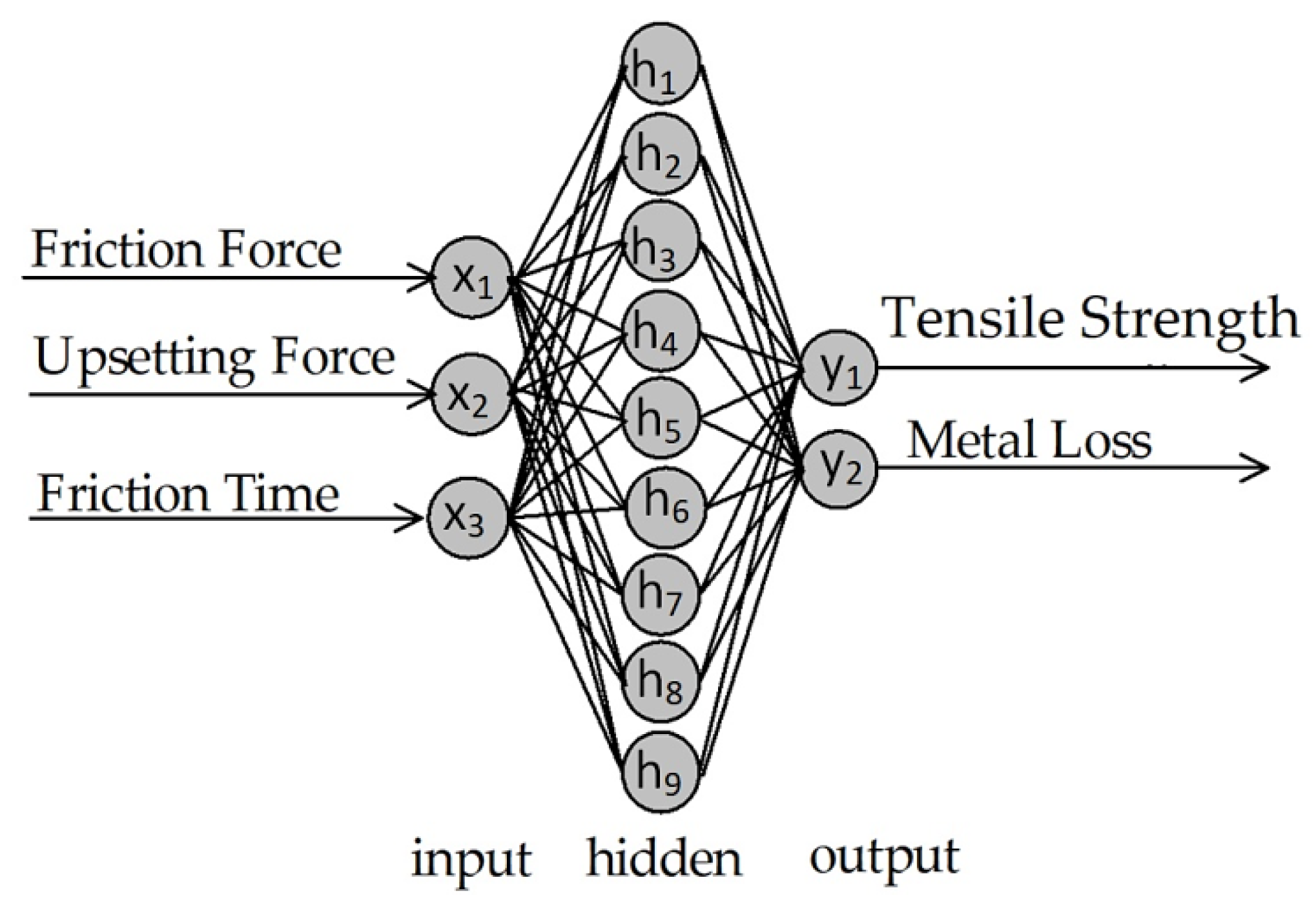
The typical architecture of an ANN includes an input layer, one or more hidden layers, and an output layer. The layers consist of one or more neurons linked together by weights and biases. In this study, a multilayer perceptron of ANN architecture is shown in Figure 4. The optimum architecture is taken as 3-9-2: three neurons in the input layer FF (x₁), UF (x₂), and FT (x₃), nine neurons in the hidden layer and two neurons in the output layer UTS (y₁) and ML (y₂). Logarithmic–sigmoidal activation functions for the hidden and output layers were selected for the study.

4.2. Validation and Learning Process

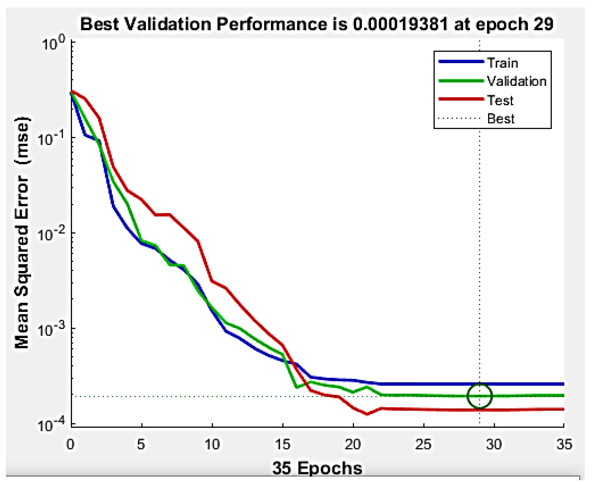
The relationship between process parameters and the tensile strength of the joint and the shortening of materials were modelled using artificial neural networks (ANNs) in Matlab. In this case study, a multilayer neural network with a backpropagation algorithm used the Lavenberg Marquart method for learning data [47]. The best MSE for the validation test is shown in Figure 5.

The best fit was obtained after 29 epochs, for which the smallest MSE error was 0.00019381. The low value of the mean squared error indicates that the neural network model developed will provide good predictions.

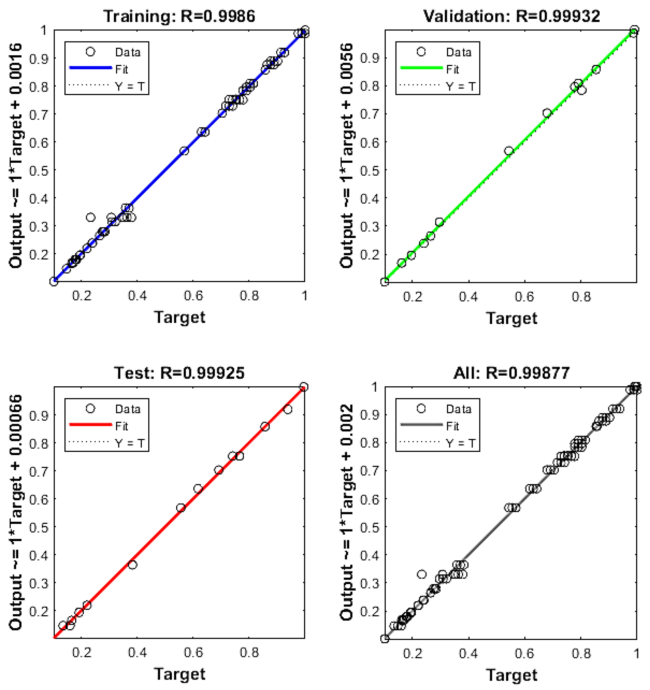
Figure 6 shows the performance plot for training, validation, testing and overall data. A correlation coefficient (R-value) close to 1 implies a close relationship between definite output and forecast output.

Figure 6 shows the results of the correlation coefficient R for the training, test, validation and total sets. The values for these sets are 0.9986, 0.9993, 0.9992 and 0.998, respectively. These values are close to 1; hence, it can be concluded that the neural network has been well-modelled and can be used to optimise the process parameters [47].

4.3. Formulation of Objective Function

The objective functions for ultimate tensile strength (UTS) and metal loss (ML) are calculated as follows:

$$\begin{array}{l}\mathrm{Maximise}\mathrm{T}\mathrm{S}\\ =\left({\displaystyle \frac{1}{1+e^{-(-2.48\times \mathrm{F}1+3.49\times \mathrm{F}2-3.97\times \mathrm{F}3-4.41\times \mathrm{F}4+3.57\times \mathrm{F}5-1.46\times \mathrm{F}6+2.59\times \mathrm{F}7+1.19\times \mathrm{F}8+1.05\times \mathrm{F}9+3.30)}}}\right)\end{array}$$

(1)

$$\begin{array}{l}\mathrm{Minimise}\mathrm{M}\mathrm{L}\\ =\left({\displaystyle \frac{1}{1+e^{-(-0.82\times \mathrm{F}1+1.72\times \mathrm{F}2-0.80\times \mathrm{F}3-6.62\times \mathrm{F}4+0.04\times \mathrm{F}5-1.18\times \mathrm{F}6-2.62\times \mathrm{F}7-6.37\times \mathrm{F}8+15.97\times \mathrm{F}9+6.90)}}}\right)\end{array}$$

(2)

The mathematical formulations (1) and (2) can be derived from resulting weights and activation function (3).

The activation function was given as

$$E_i=\left({\displaystyle \frac{1}{1+e^{-T_i}}}\right),$$

(3)

Function (3) determines the value of the state of the neurons, which will be transmitted to the downstream neurons.

• where

$$T_i=w_1{\times x}_1+w_2\times x_2+w_3\times x_3+b$$

(4)

The constants used to estimate the $T_i$ are given in

Table 7. Weights (w_i) and biases (bi) derived from input and hidden layer of neural network.

i	${\mathit{w}}_1$	${\mathit{w}}_2$	${\mathit{w}}_3$	$\mathit{b}$
1	$32.06$	$43.76$	$9.00$	$-75.68$
2	$-11.04$	$1.27$	$-22.02$	$28.69$
3	$-30.41$	$41.24$	$-9.48$	$4.66$
4	$-23.66$	$19.73$	$-27.44$	$25.19$
5	$-28.80$	$46.06$	$3.44$	$-17.64$
6	$-22.36$	$-33.61$	$22.25$	$33.11$
7	$-8.82$	$44.44$	$-18.80$	$-20.31$
8	$6.98$	$-37.82$	$16.70$	$14.74$
9	$-12.07$	$41.93$	$16.38$	$-47.43$

.

In this study, functions (1)–(4) are simultaneously optimised according to the lower and upper bounds, as shown below:

$${35\le \mathrm{x}}_1\le 45$$

(5)

$$40\le {\mathrm{x}}_2\le 50$$

(6)

$$6\le {\mathrm{x}}_3\le 12$$

(7)

The constraints in Equations (5)–(7) are the constraints for the friction force x₁, the upsetting force x₂ and the friction time x₃, respectively.

4.4. Genetic Algorithms

Recently, many works have been devoted to multi-criteria optimisation using genetic algorithms. The most popular are the multi-criteria genetic algorithms MOGA and NSGA. Both methods provide solutions in the form of a Pareto chart. These algorithms are an optimisation method based on the natural evolution of populations of living organisms. The algorithms conduct searches on populations built of chromosomes. These, in turn, are built of genes. Genetic algorithms search for the best solutions from a population and not from a single point. Genetic algorithms use random methods of chromosome selection in which crossover and mutation operators play an important role. Crossover is the exchange in a sequence of genes between two chromosomes. A mutation parameter involves changing the value of a gene in a single chromosome [48]. Genetic algorithms optimise tasks in a big search space for nonlinear functions of complex problems.

A multi-objective genetic algorithm (MOGA) is employed to optimise engineering tasks where multiple criteria impact the quality of the solutions. MOGA identifies a set of decision variables that meet specific constraints to provide satisfactory values for all objective functions. The algorithm minimises or maximises several objective functions [46,48]. MOGA produces a set of optimal solutions known as Pareto optimal solutions. The Pareto front represents all of these non-dominated solutions within the objectives space. This study used the Non-Sorting Genetic Algorithm II (NSGA-II) for the multi-objective optimisation of process parameters. The main steps of the NSGA-II have been demonstrated in previous papers [49,50].

Multi-objective optimisation was performed using the Gamultiobj procedure in the Optimisation Tool of Matlab R2018a software. Gamultiobj uses the NSGA II for multi-objective optimisation [47,51]. The main parameters of the multi-objective genetic algorithm are presented in

Table 8. NSGA-2 main parameters.

GA Parameter	Symbol	Value
Number of generations	Ng	500
Population size	Pop.size	80
Crossover function	Cf	heuristic
Crossover probability	Cprob	0.9
Mutation function	Mf	uniform
Mutation probability	Mprob	0.2

.

5. Results and Discussion

Table 9. The predicted Pareto results of tensile strength and metal loss.

No.	FF (kN)	UF (kN)	FT (s)	TS (MPa)	ML (mm)
1	35	40	9	30.06	0.23
2	35	48	6	80.13	8.25
3	35	48	8	79.76	7.84
4	35	41	9	44.23	0.30
5	35	42	11	78.81	5.34
6	35	40	9	33.37	0.24
7	35	42	10	78.62	4.81
8	35	42	10	78.18	3.94
9	35	42	10	77.41	2.93
10	35	42	10	76.72	2.30
11	35	40	9	40.44	0.29
12	35	48	8	79.39	7.60
13	35	42	10	72.92	1.19
14	35	42	10	75.98	1.94
15	35	42	10	75.36	1.86
16	35	41	9	54.99	0.40
17	35	41	9	52.85	0.38
18	35	42	10	77.04	2.76
19	35	42	11	79.17	7.03
20	35	42	11	78.89	5.77
21	35	40	9	40.44	0.29
22	35	42	10	73.98	1.35
23	35	42	10	77.72	3.28
24	35	42	10	74.25	1.54
25	35	41	9	49.89	0.34
26	35	42	10	78.42	4.42
27	35	48	7	80.07	8.18
28	35	42	10	71.42	0.94
29	35	42	11	78.81	5.34
30	35	41	9	58.62	0.43
31	35	42	11	78.93	6.06
32	35	42	11	79.10	6.63

shows the thirty-two solutions (No. 1–32) of the optimal set in the Pareto sense.

Table 9 shows that the best solutions were obtained for a low friction force of 35 kN and a friction welding time of 10 s. According to the results (see Table 9, No. 7–10), the tensile strength was about 80 MPa, and the average joint shortening was only 3.5 mm. For these solutions, the upsetting force was also low. Increasing the upsetting force to almost the maximum value (48 kN) caused more significant material losses of up to 8 mm. It is worth noting that in the optimisation case, a lower material loss of about 50% was achieved, comparing Table 4, No. 7, 8 with Table 9, No. 7, 8.

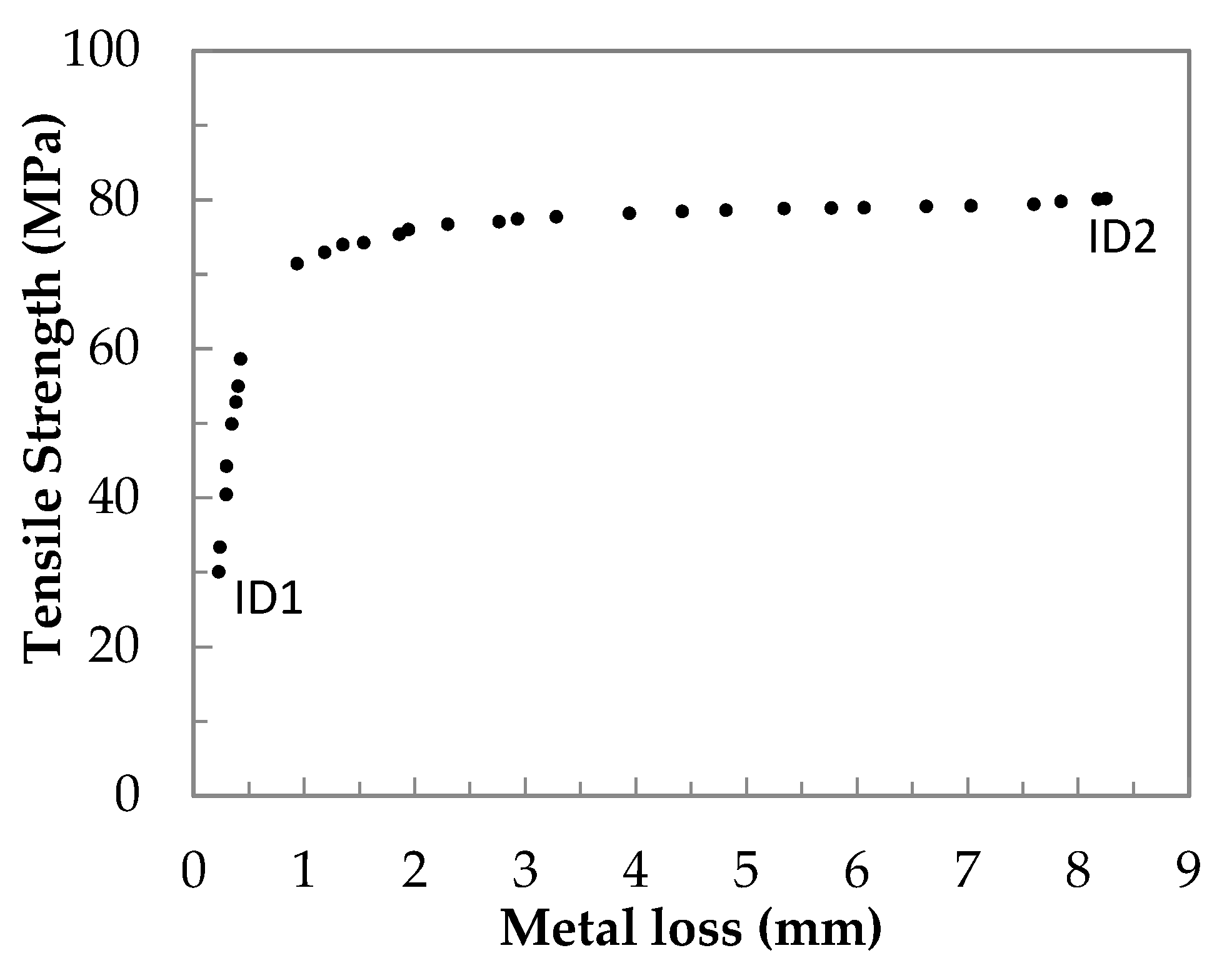
The Pareto curve of UTS and ML using genetic algorithms is presented in Figure 7.

The set of solutions consists of 32 points, forming a Pareto curve, with limits defined by the extreme points ID1 and ID2 (see No. 1 and 2, Table 9). Point ID2 in Figure 7 is the highest point on the Pareto curve with the highest UTS = 80.13 MPa and the highest metal loss ML = 8.25 in mm (see Table 9, point No. 2). For point ID2, the welding parameters are as follows: friction force is 35 kN, friction time is 6 s, and upsetting force is 48 kN. The lowest point on the Pareto curve is ID1 (see Figure 7). For point ID = 1, the lowest metal loss is 0.23 mm, while the lowest UTS = 30 MPa is received (see No. 1 in Table 9). For point ID1, the following welding parameters (FF = 35 kN, FT = 9 s and UF = 40 kN) were found. When the Pareto solutions are analysed further, more information regarding the variation in the process parameters is exposed. All the Pareto solutions are numbered and sorted in order to increase the tensile strength of the joint and decrease metal loss for all cases.

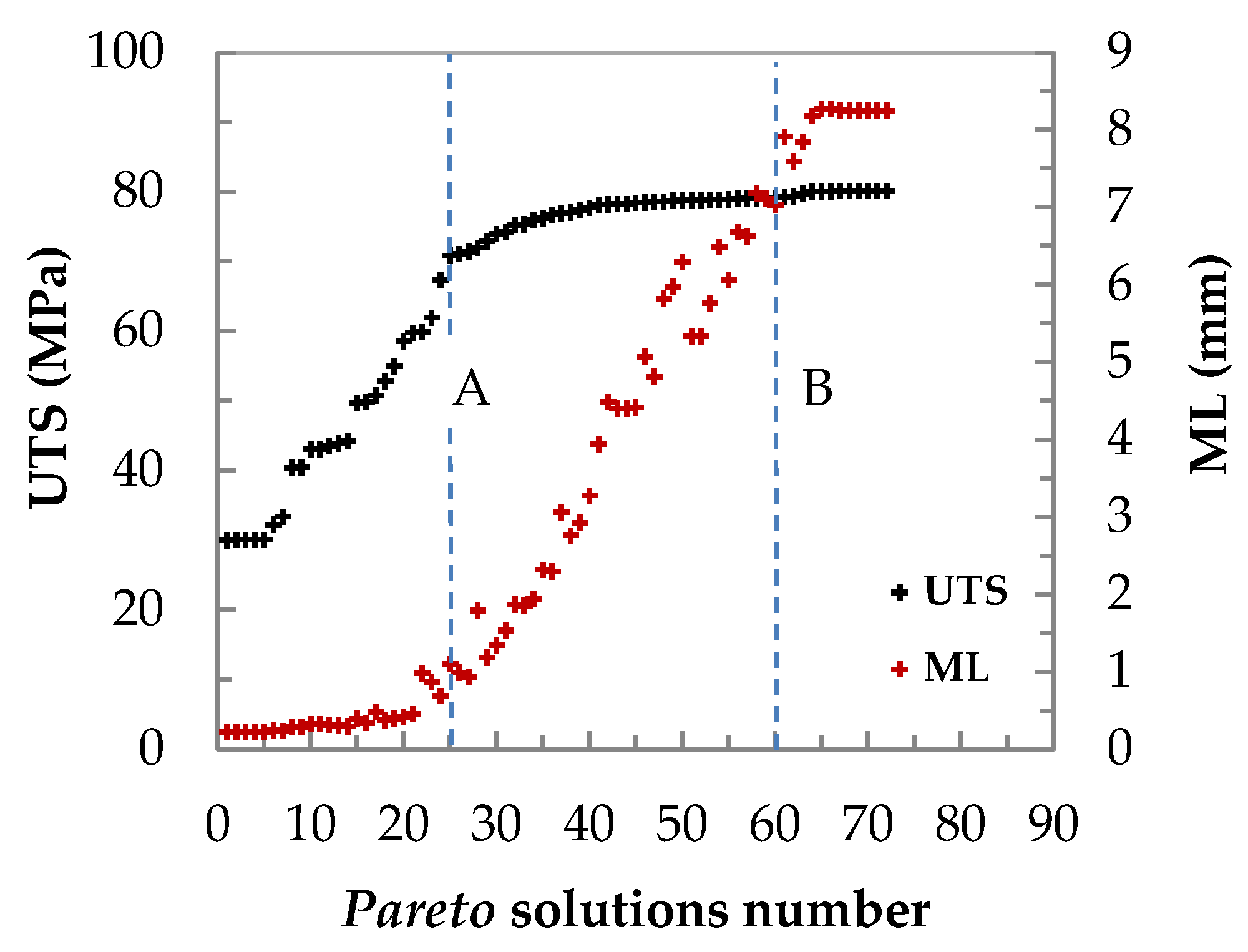
Figure 8 shows the variation in UTS and ML values of the Pareto solutions for the AZ91D/6061 joint (arranged in ascending order and plotted as the population size (Pop_size).

Conflicting relations between the objective functions (UTS and ML) of welding process quality have been observed. The Pareto solution number of UTS vs. ML was optimised using a combination of Ngen and population size. In this optimisation task, the N_gen and Pop_size values were 80. The probability crossover of 0.9 and mutation of 0.2 are kept constant in all optimisation procedures. In this problem, the UTS and ML were optimised simultaneously. However, finding a solution that simultaneously optimises UTS and ML is not possible. From Figure 8, it can be observed that the range of region (A–B) of higher UTS (68–80 MPA) with metal loss that changed in the range (0.7–7 mm) was selected for further analysis of the Pareto results. The solution numbers corresponding to the region (A–B) are 25 to 60, which could be used to determine the ranges of best FF, FT, and UF welding parameters.

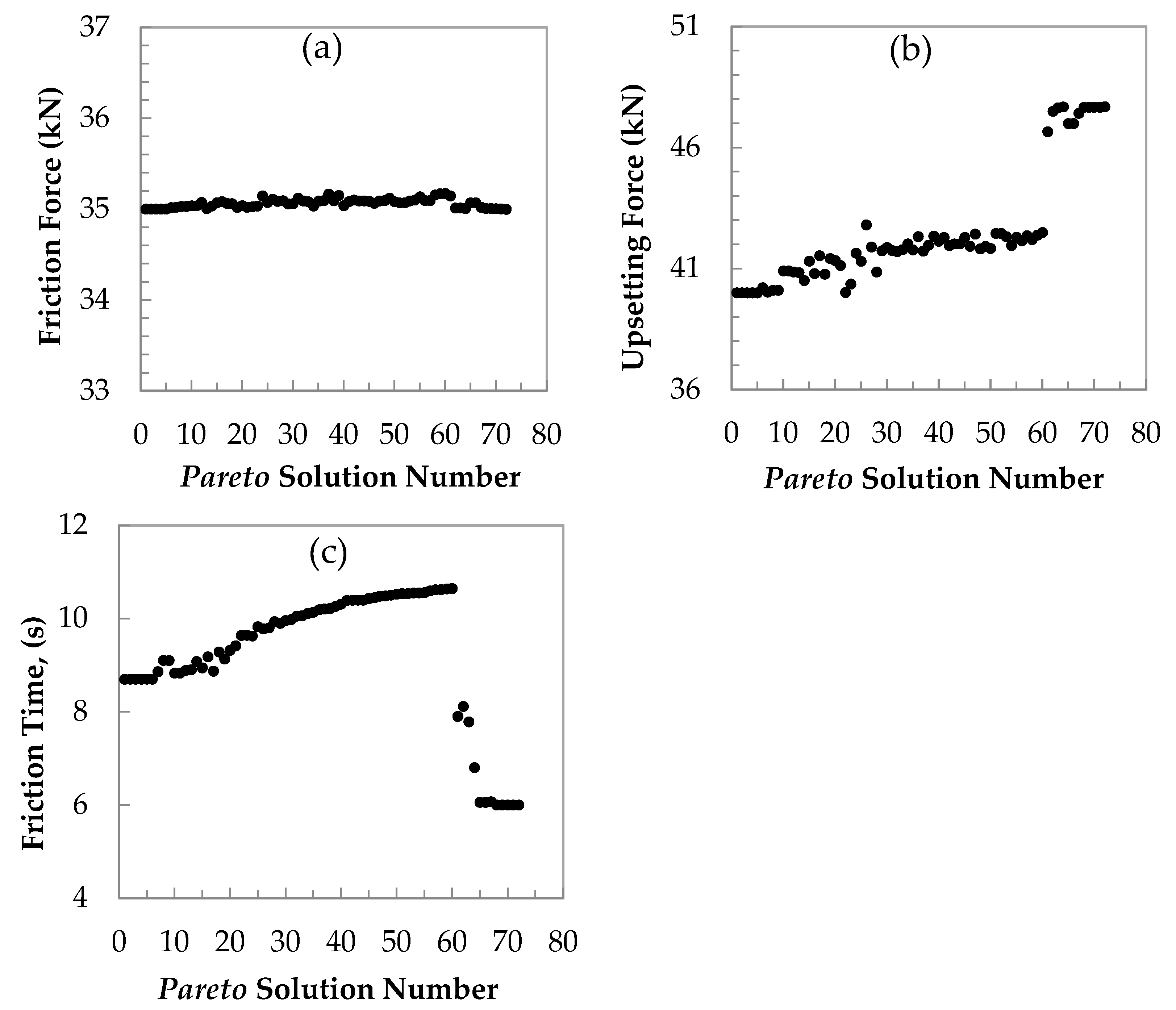
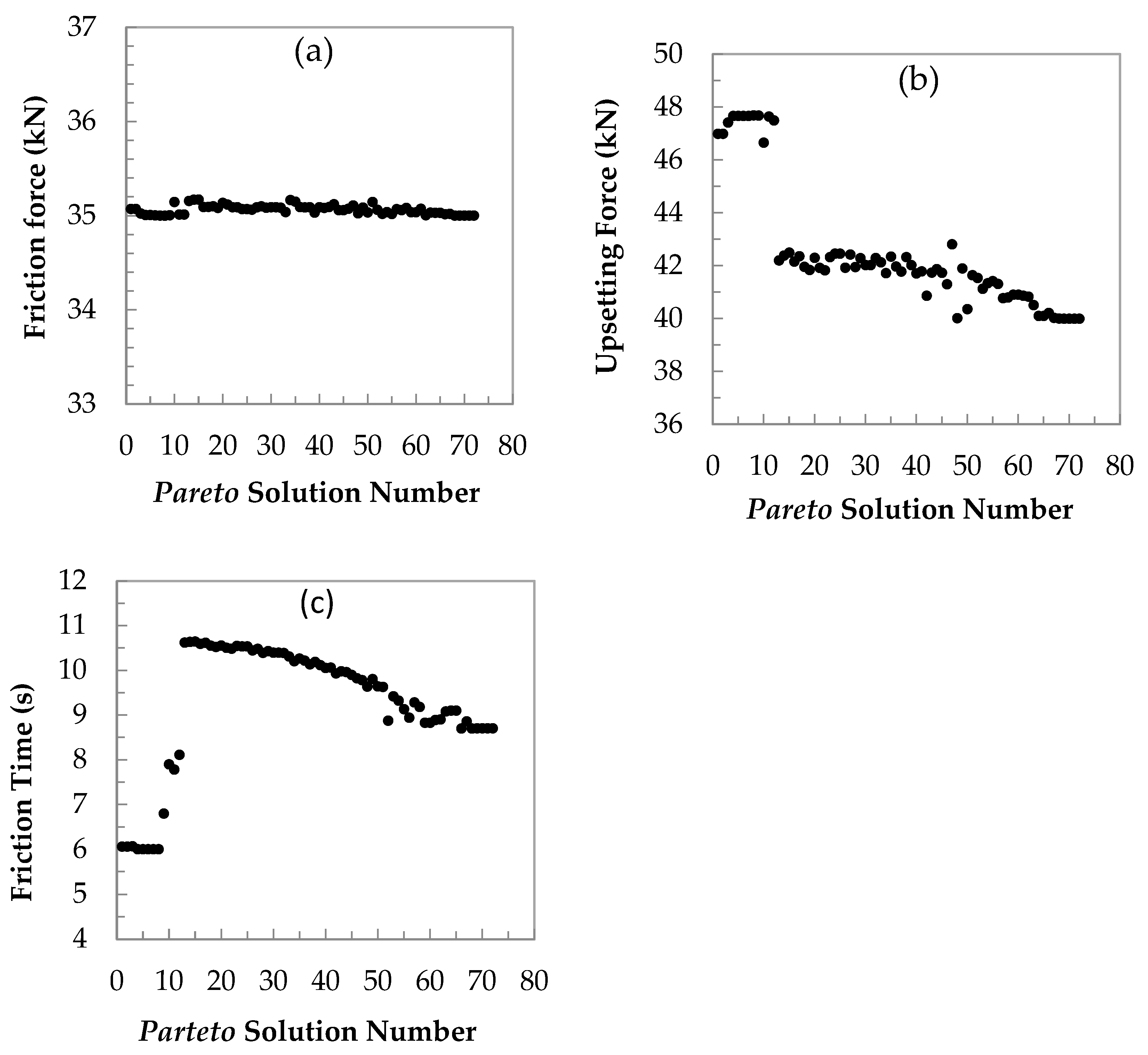
The process parameter solutions FF (a), UF (b) and FT (c) in all 80 Pareto solutions with increasing tensile strength are shown in Figure 9.

The optimisation results in Figure 9 show many variants of Pareto solutions for welding parameters. Figure 9a indicates the average value of 35 kN for FF, whereas UF increases linearly from 67 to 80 MPa (Figure 9b). Figure 9b,c show the increasing UF and UT values in the A–B range. Moreover, the constant values outside the range are visible. The UF and UF values are 48 kN and 6 s, respectively.

Figure 10 shows the variation in the FF, UF and FT parameters in all 80 Pareto solutions with decreasing metal loss.

Figure 10 shows the predicted effects of friction force, upsetting force and friction time on the metal loss in the Pareto solution number. As expected, with increasing upsetting force and more shortening of metal in the considered area (A–B), UF decreases linearly from 42 to 40 kN, or logarithmically from 27 to 46%. After reaching 60 generations, the shortening value stabilises at an 8 mm level. The predicted pattern shows linearly decreasing metal loss with decreasing upsetting force and friction time [52,53].

The new experimental runs for FF = 35 kN, UF = 48 kN, and FT = 6 s were used to confirm the developed model. The validation UTS and ML results are presented in

Table 10. Validation results.

	UTS	ML
$\mathrm{Experimental} \mathrm{values} (y_{ei}$)	82	8.50
$\mathrm{Predicted} \mathrm{values} (y_{pi}$)	80	8.25
$\mathrm{Errors}={\displaystyle \frac{y_{ei}-y_{pi}}{y_{pi}}}·100$%	2.4	3.0

.

Table 10 shows that the experimental values are close to those obtained by the genetic algorithm. So, the absolute relative error between them was only 3%.

6. Conclusions

In the present study, the first sound joint was attained between the AZ91D magnesium alloy and AA6082 aluminium alloy using a conventional friction welding method. Additionally, a new approach in multi-criteria optimisation of welding parameters was presented to obtain maximum joint strength and minimum shortening of joints. The following conclusions can be drawn from the research:

• A neural network with nine neurons in the hidden layer and a log-sigmoidal activation function were the best approximators in formulating a multi-objective function for the genetic algorithm.
• The NSGA-2 genetic algorithm found a set of welding parameters for which the joint strength increases from 24 to 81 MPA, and the joint shortening decreases from 8.25 to 0.23 mm. These solutions are in constant conflict with each other.
• The increase in welding time and upsetting force has a positive effect on the increase in the tensile strength of the welded joint and a negative effect on material losses.
• The results show that a low friction force (35 kN) and upsetting force (42 kN) give a high value of tensile strength (78 MPa) and the lowest shortening (3.5 mm) of the bimetal joints.
• During the verification of the model for the new welding parameters, its error did not exceed 3%.

This study can be extended to the microstructure and crack behaviour at the joint interface. The influence of welding parameters on the formation of intermetallic compound (IMC) layers and microcracks, reported in the references [42,43,44] for this pair of joined materials, should be investigated.