Article

New Hybrid Approaches Based on Swarm-Based Metaheuristic Algorithms and Applications to Optimization Problems

by
Mustafa Serter Uzer
Electronics and Automation, Ilgın Vocational School, Selcuk University, Konya 42600, Turkey
Appl. Sci. 2025, 15(3), 1355; https://doi.org/10.3390/app15031355
Submission received: 31 December 2024 / Revised: 25 January 2025 / Accepted: 26 January 2025 / Published: 28 January 2025
(This article belongs to the Section Computing and Artificial Intelligence)

Abstract

:
Metaheuristic algorithms are favored for solving a variety of problems due to their inherent simplicity, ease of implementation, and effective problem-solving capabilities. This study proposes four new hybrid approaches using swarm-based metaheuristic algorithms. Two of these new approaches are HHHOWOA1 and HHHOWOA2, based on the hybridization of Harris Hawks Optimization (HHO) with the Whale Optimization Algorithm (WOA), and the others are HHHOWOA1PSO and HHHOWOA2PSO, based on the hybridization of HHHOWOA1 and HHHOWOA2 with particle swarm optimization (PSO). An evaluation of these four innovative approaches is conducted on 23 benchmark functions, and their results are compared to those reported in the literature under equivalent parameter settings. Among the four approaches, HHHOWOA1 and HHHOWOA2PSO have demonstrated more favorable results. According to the literature, the HHHOWOA1 and HHHOWOA2PSO approaches achieve the most optimal results, either better or with the same average fitness values in 15 of the 23 functions and in 18 of the 23 functions, respectively. Moreover, the proposed approaches have been applied to three engineering problems, and the optimum values obtained are compared to the literature. Ultimately, the proposed approaches have proven effective in providing competitive solutions for the majority of optimization problems.

1. Introduction

In recent years, the increasing complexity of theoretical and practical problems in different fields has increased the need for researchers to propose further improved optimization methods [1]. Optimization problems are always important and challenging in engineering design, particularly accuracy design optimization, as demonstrated in [2]. To find the best solution, optimization methods can either employ stochastic or deterministic approaches [3,4]. Stochastic approaches are typically categorized alongside heuristics and metaheuristics [3,4,5]. Metaheuristic approaches (MHAs) are used for various problems because of their simplicity, ease of implementation, and problem-solving power. Especially, MHAs are successfully used to solve benchmark functions and engineering problems in various disciplines [6]. Furthermore, these techniques may be used to update the weight values of the network in Artificial Neural Networks (ANNs) [7] to generate optimum solutions in fuzzy-based optimization algorithms [8,9,10] or to choose ideal subsets in binary feature selection [11].
The creation of MHAs is motivated by various factors, including natural evolution, electromagnetic force, humans, plants, animals, and ecosystems [12]. In the literature, MHAs have been classified in a variety of ways. In one of these categorizations, MHAs are divided into population-based and single-based groups [13]. The fundamental concept of single-based metaheuristic algorithms, additionally referred to as trajectory algorithms, is that a single solution is created for each iteration. This solution is improved by using the neighborhood technique. Examples of well-known single-based MHAs [13] are Iterated Local Search (ILS) [14], Simulated Annealing (SA) [15], and Guided Local Search (GLS) [16]. In contrast to single-based MHAs, population-based MHAs present a group of solutions during each run. Population-based MHAs may be classified into four types [17]: swarm-based, human-based, evolutionary-based, and physics-based.
Swarm-based MHAs, which have an important place in the literature, model the swarm behavior’s intelligent features [18] and use the natural world’s collective behaviors as their information source (for instance, birds, bees, and ants). The literature examples for the swarm-based category include the Tunicate Swarm Algorithm (TSA) [19], the Artificial Bee Colony (ABC) [20], the Butterfly Optimization Algorithm (BOA) [21], Harris Hawks Optimization (HHO) [17], the Emperor Penguin Optimizer (EPO) [22], particle swarm optimization (PSO) [23], the Optimal Foraging Algorithm (OFA) [24], Grey Wolf Optimization (GWO) [25], the Grasshopper Optimization Algorithm (GOA) [26], the Salp Swarm Algorithm (SSA) [27], the Whale Optimization Algorithm (WOA) [28], and the Crow Search Algorithm (CSA) [29].
Researchers have recommended tactics to increase the performance of their optimization algorithms, such as providing new algorithms, improving existing ones, and combining several approaches [30,31]. The most well-known methods or hybrid optimization methods are listed below. The Harris Hawks Optimizer (HHO) simulates the situation in which many hawks collaborate to attack their prey from various angles [17]. Hawks have evolved hunting strategies depending on their prey’s attempts to flee. The HHO method has been evaluated in a variety of benchmarks and engineering issues, and the findings suggest that it outperforms previous techniques [17]. Nonetheless, HHO has some faults, such as local optimality, premature convergence, and performance loss for high-dimensional problems [32]. The following are some of the publications in the literature that use the HHO algorithm. For multi-level picture thresholding, Leader Harris Hawks Optimization (LHHO) has been developed to increase HHO’s exploration capabilities [33]. Improved HHO is presented in [34] to conduct global optimization and select the optimal threshold values for multi-level picture segmentation challenges. Furthermore, HHOSSA, an enhanced HHO that considers the SSA, is suggested, and this work has produced a multi-level picture segmentation technique. The Grasshopper Optimization Algorithm (GOA), a novel swarm intelligence approach, was inspired by grasshopper foraging and swarming behavior in the outdoors [26]. The GOA approach has demonstrated its worth in the literature by efficiently addressing a wide range of optimization issues in a variety of domains [13]. The Grey Wolf Optimization (GWO) optimization approach replicates grey wolf hunting methods in the wild [25]. GWO is based on group hunting methods used by grey wolves as part of their social systems. The ABC algorithm was developed by modeling the foraging behavior of honey bees [20], and it has been utilized to solve many different engineering problems so far [35,36]. Combining HHO and the African Vulture Optimization Algorithm (AVOA), a hybrid HHO-AVOA optimization method is introduced in [37]. It addresses path-planning challenges for differential wheeled mobile robots (DWMRs) in static and dynamic environments, considering kinematic constraints. The HHO with Memory-Saving Strategy (HHO-MSS) optimization method is introduced [38]. This new method for optimizing the parameters of the Power System Stabilizer and Virtual Inertia in a renewable microgrid power system with diverse energy sources is suggested. The RSRFT approach was developed by integrating the Reptile Search Algorithm (RSA) with the Red Fox Algorithm (RFO) and the Triangular Mutation Operator (TMO) [39]. This method was optimized to enhance the exploration and exploitation phases. An enhanced dung beetle optimization algorithm (EDBO) has been introduced to address nonlinear optimization challenges with multiple constraints in manufacturing [40]. The algorithm’s ability to explore and exploit is strengthened by refining its rolling, dancing, and foraging processes. To address the low convergence accuracy and the tendency to fall into the local optima of the traditional Harris Hawks Optimization (HHO) algorithm, a Compound Improved HHO (CIHHO) is proposed [41]. Enhancements include the dynamic adjustment of energy, the Versoria function for improved local exploration, Levy flight for escaping local optima, and random white noise for increased accuracy. A hybrid optimization algorithm (HSSOGSA) that combines the exploitation capability of Sperm Swarm Optimization (SSO) with the exploration capability of the Gravitational Search Algorithm (GSA) is proposed [42]. This study demonstrates that the hybrid method outperforms the standard SSO and GSA in terms of faster convergence and better ability to escape local extremes across most benchmark functions.
The Whale Optimization Algorithm (WOA) is an algorithm that simulates humpback whale hunting stages [28]. The WOA is based on the fact that humpback whales encircle and catch their prey in a smaller area due to the air bubbles they create. The Moth–Flame Optimization (MFO) algorithm has been proposed, inspired by a moth’s navigation method in nature [43]. Five algorithms consisting of different combinations of the WOA, PSO, and Levy flight are proposed in [5]. The best of these five algorithms, the WOALFVWPSO algorithm, was compared to the literature for 23 benchmark and pressure vessel design problems, and it was found that this algorithm produced more competitive solutions for most problems. A novel wrapper-based feature selection approach, referred to as BWPLFS, is introduced, combining binary WOA, PSO, and Lévy flight in [11]. The method is evaluated using 10 benchmark datasets and compared against various algorithms from the literature. The results indicate that the proposed method effectively identifies the most relevant features. The hybrid SCWOA method, which is based on the WOA with SCA, is proposed for evaluating benchmark functions and engineering designs, aiming ultimately to determine the global optimal values of the functions and the associated costs of the designs [44]. The hybrid hPSO-TLBO approach, based on a combination of particle swarm optimization (PSO) and teaching–learning-based optimization (TLBO), is proposed to solve optimization problems [45]. The core concept of the hPSO-TLBO design is to merge PSO’s exploitation capability with TLBO’s exploration strength.
As a result, the development of optimization methods is essential to provide more efficient and effective solutions from both theoretical and practical perspectives. Swarm-based methods still have potential for further development, and hybrid innovative approaches can enhance performance. Therefore, this study proposes four new hybrid approaches.
This article’s significant contributions are as follows:
  • Based on HHO, the WOA, and PSO, this work has presented four novel hybrid approaches dubbed HHHOWOA1, HHHOWOA2, HHHOWOA1PSO, and HHHOWOA2PSO.
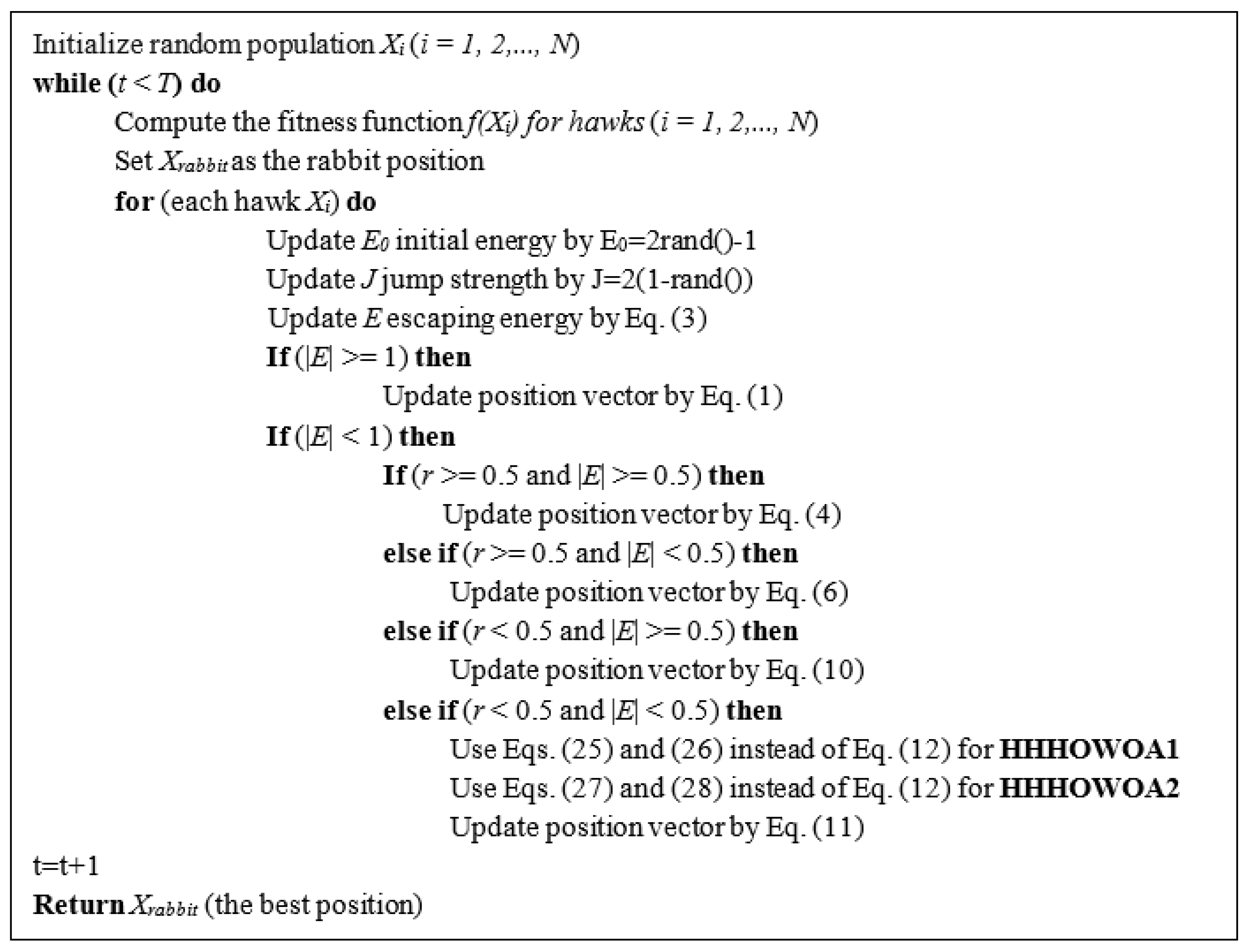
  • The HHHOWOA1 and HHHOWOA2 methodologies are developed by modifying the equations utilized in the exploitation phase of the WOA and subsequently applying these modifications in the exploitation phase of Harris Hawks Optimization (HHO). The HHHOWOA1PSO and HHHOWOA2PSO methodologies are developed by using modified PSO equations during the final stages of the HHHOWOA1 and HHHOWOA2 algorithms. Both the WOA and HHO algorithms have been improved because of these new hybrid techniques.
  • The general problems of metaheuristic algorithms that often involve getting stuck in local optima, low diversity, and imbalanced exploitation capabilities have been further improved. So, the optimization search capability has been further improved, and the probability of the optimal value falling to a local minimum has been further reduced.
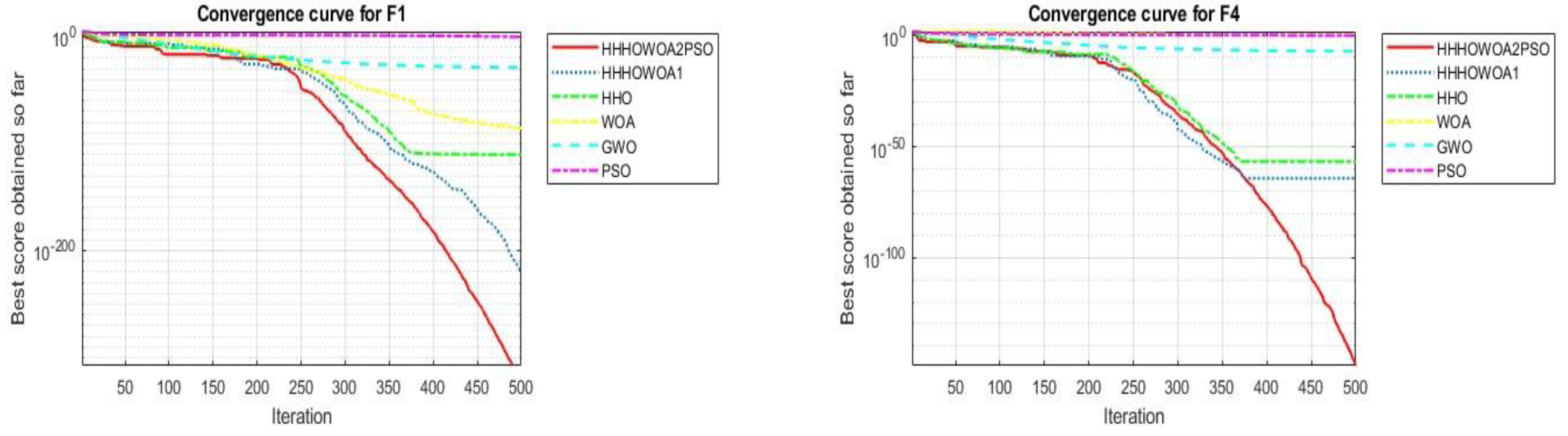
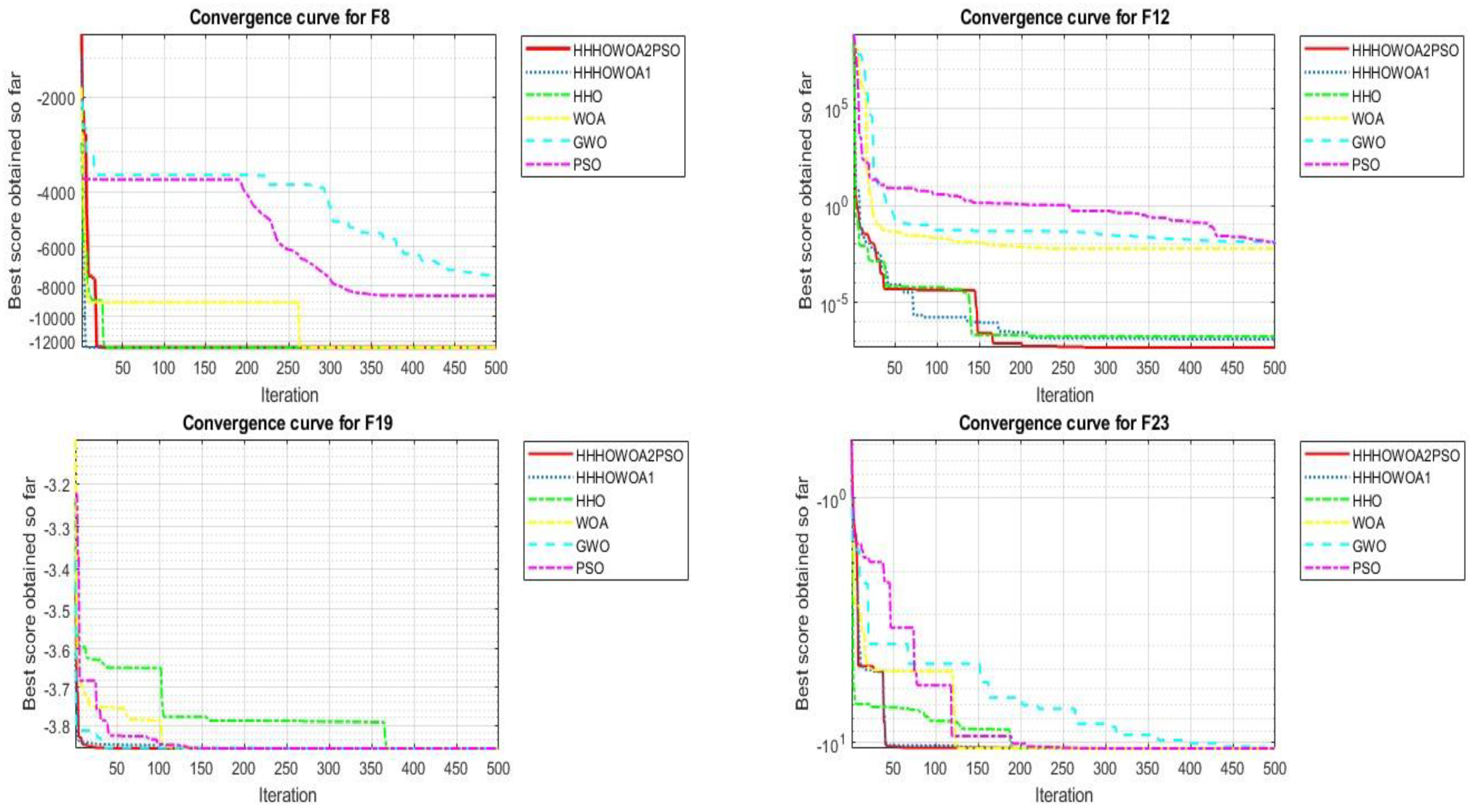
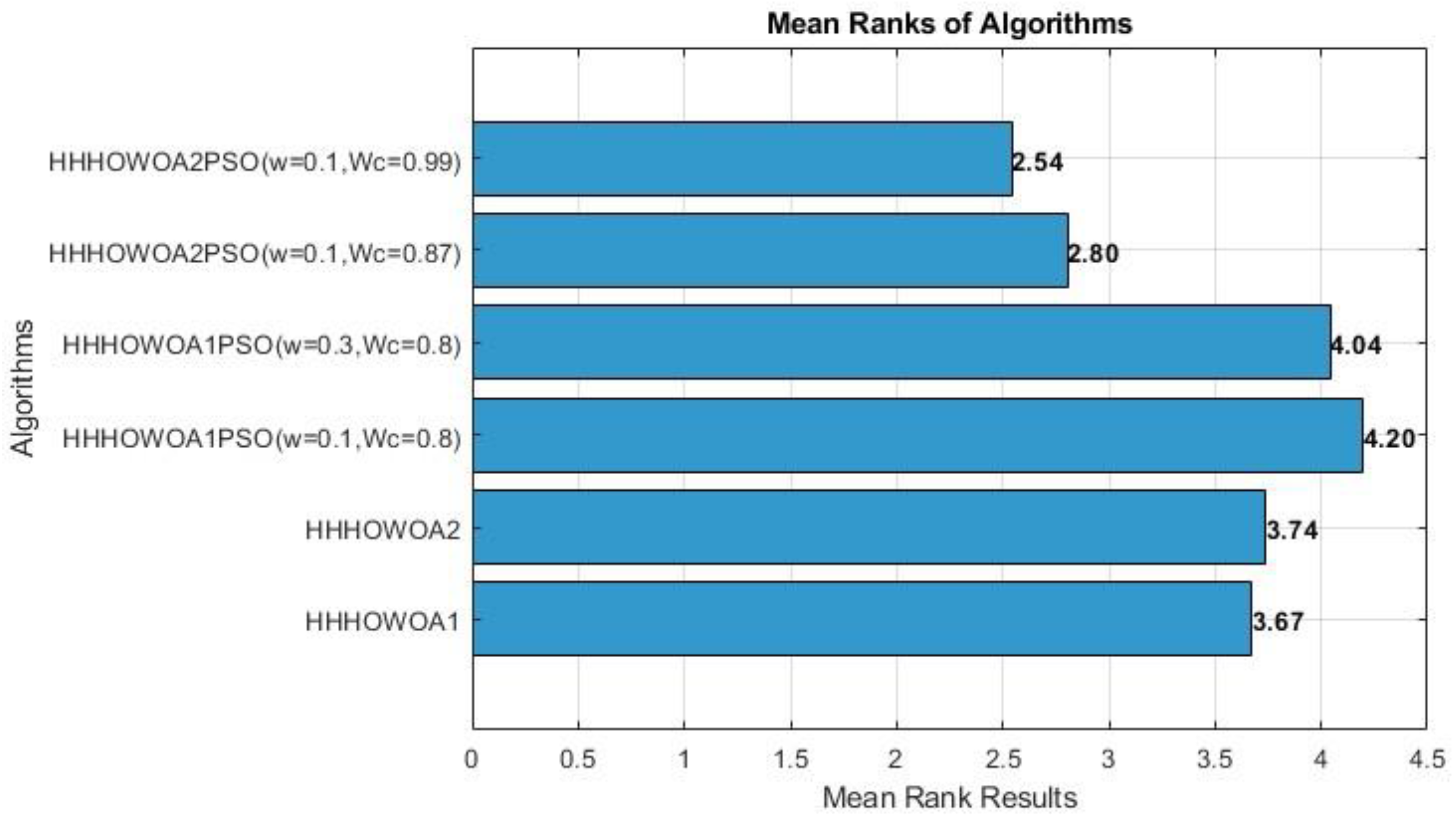
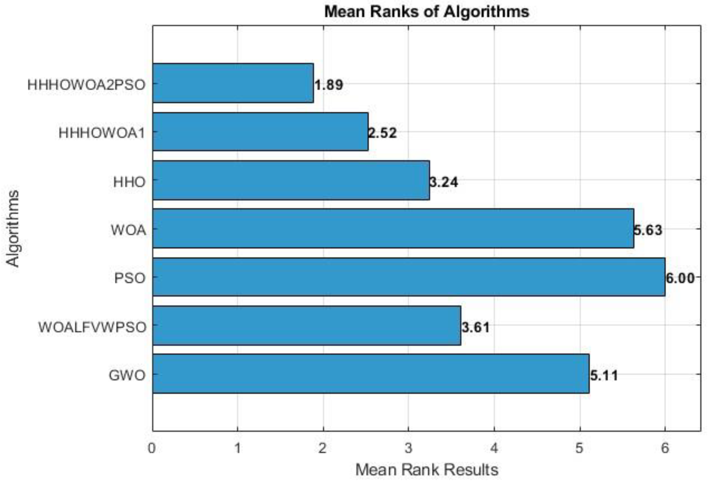
  • The proposed four novel hybrid approaches were evaluated on 23 benchmark functions and compared to the results of the publications using the same parameters. For these 23 functions, Friedman rank tests were performed based on the average optimization results of all algorithms. It was observed that the HHHOWOA2PSO approach is ranked first, followed by the HHHOWOA1 approach, in the success ranking for the F1–F23 functions.
  • The HHHOWOA1, HHHOWOA2, and HHHOWOA2PSO approaches are applied to three benchmark problems in engineering, and the optimum values obtained are compared with the literature.
The structure of this manuscript is as follows: Section 2 introduces the HHO algorithm and its steps, the WOA algorithm and its steps, as well as the PSO method. Section 3 provides a detailed explanation of the proposed algorithms. Section 4 includes the benchmark sets, comparisons of the proposed algorithms with each other and with the existing literature, statistical analyses, and the application of the proposed approaches to three engineering problems. Finally, Section 5 concludes this study by summarizing the key findings.

2. Preliminaries

2.1. Harris Hawks Optimization (HHO)

The HHO method is an optimization approach that imitates the action of numerous hawks cooperating to attack from different angles in order to confuse prey [17]. In response to their prey’s escape methods, hawks have evolved a range of hunting approaches. HHO is produced by the mathematical modeling of these various techniques, and the steps of HHO are listed below.

2.2. Exploration Phase of HHO

The Harris’s hawks in HHO perch in various locations and wait for prey to show up using one of two strategies utilizing Equation (1).
X ( t + 1 ) = X r a n d ( t ) r 1 X r a n d ( t ) 2 r 2 X ( t ) q 0.5 ( X r a b b i t ( t ) X m ( t ) ) r 3 ( L B + r 4 ( U B L B ) ) q < 0.5
where r1, r2, r3, r4, and q variables are random numbers inside (0, 1). Xrand (t), Xrabbit (t), X (t), Xm, and X (t + 1) represent the random hawk population, the rabbit’s position, the hawks’ present position, the hawk population’s mean position, and the hawks’ next position vector, respectively. The variables’ upper and lower limits are expressed as LB and UB, respectively. Xm is calculated using Equation (2).
X m ( t ) = 1 N i = 1 N X i ( t )
where N and Xi (t) represent the hawks’ total number and each hawk in iteration t, respectively.

2.3. Exploration to Exploitation Transition of HHO

By using Equation (3), the rabbit’s energy is calculated.
E = 2 E 0 1 t T
where T and E0 represent the maximum iteration and the rabbit’s energy beginning state.

2.4. Exploitation Phase of HHO

There are four stages of besiege at this phase. The first of these stages is the soft besiege. This besiege is performed by using Equations (4) and (5).
X ( t + 1 ) = Δ X ( t ) E J X r a b b i t ( t ) X ( t )
Δ X ( t ) = X r a b b i t ( t ) X ( t )
where the rabbit’s randomized leap power is denoted by J = 2 × (1 − r5) during the escaping process and r5 is a random number in (0, 1).
The second stage of the exploitation phase is the hard besiege. This besiege is performed with Equation (6).
X ( t + 1 ) = X r a b b i t ( t ) E Δ X ( t )
The third stage of the exploitation phase is the soft besiege with progressive rapid dives. In this stage, the next move for the soft besiege is performed with Equation (7).
Y = X r a b b i t ( t ) E J X r a b b i t ( t ) X ( t )
In this stage, a dive move based on LF is performed with Equation (8).
Z = Y + S × L F ( D )
where S is 1 × D random vector, D is the problem’s dimension, and LF (levy flight) is calculated with Equation (9) [17].
L F ( x ) = 0.01 × u × σ v 1 / β ,   σ = Γ ( 1 + β ) × sin ( π β 2 ) Γ ( 1 + β 2 ) × β × 2 ( β 1 2 ) 1 / β
where u and v are random values in (0, 1), and where β parameter is 1.5. The hawks’ positions are updated with Equation (10).
X ( t + 1 ) = Y i f   F ( Y ) < F ( X ( t ) ) Z i f   F ( Z ) < F ( X ( t ) )
Here, Equations (7) and (8) are used to calculate Y and Z.
The last stage of the exploitation phase is hard besiege with progressive rapid dives. This stage is performed by Equation (11).
X ( t + 1 ) = W i f   F ( W ) < F ( X ( t ) ) V i f   F ( V ) < F ( X ( t ) )
where W and V are calculated by Equations (12) and (13). HHO’s pseudocode is given in Figure 1 [17].
W = X r a b b i t ( t ) E J X r a b b i t ( t ) X m ( t )
V = W + S × L F ( D )

2.5. Whale Optimization Algorithm (WOA)

The WOA is an algorithm that imitates the hunting stages of humpback whales [28]. The basis of the WOA is inspired by the phenomenon that humpback whales surround and collect their prey in a narrower area thanks to the air bubbles they form. The WOA imitates two stages. The exploitation phase involves surrounding a prey and using a spiral bubble-net assault technique, whereas the exploration phase involves randomly hunting for prey.

2.6. Exploitation Phase of WOA

Equations (14) and (15) imitate a whale’s behavior toward prey in the exploitation phase.
D = C X ( t ) X ( t )
X ( t + 1 ) = X ( t ) A . D
where X, X*, and t refer to the position, the best position, and the existing iteration number, respectively. The A and C coefficient vectors are calculated by Equations (16) and (17). Here, a is obtained by Equation (18) [46].
A = 2 a . r a
C = 2 . r
a = 2 t 2 T
where T refers to the maximum iteration number. The X solution is calculated by Equation (19).
X ( t + 1 ) = D e b l cos ( 2 π l ) + X ( t )
where the distance between prey and a whale is expressed as D . In addition, b constant denotes the shape of the spiral, l is a random number, and X* is the denoted best solution so far [46].
According to the random number p (0, 1), the whale chooses one of the paths using Equation (20).
X ( t + 1 ) = s h r i n k i n g   E n c i r c l i n g ( Equation ( 15 ) ) i f ( p < 0.5 ) s p i r a l   s h a p e d p a t h ( Equation ( 19 ) ) i f ( p 0.5 )

2.7. Exploration Phase of WOA

Random solutions are chosen during position regeneration [25]. To produce random values, vector A is employed. This process is expressed mathematically in Equations (21) and (22). In Figure 2, the WOA’s pseudocode is presented [28].
D = C X r a n d X
X ( t + 1 ) = X r a n d A . D

2.8. Particle Swarm Optimization (PSO)

Swarm-inspired algorithms have strong optimization capabilities, taking inspiration from the collective behavior of swarming creatures [47]. Among these, the PSO algorithm was introduced by Kennedy and Eberhart [23]. PSO imitates the social dynamics observed in animal groups, similar to groups of birds or shoals of fish. In this algorithm, each potential solution is represented as a ‘particle’ comprising a position vector and a velocity vector. Every particle modifies its position based on two key factors: its own best-found position (personal best) and the overall best position discovered by the entire swarm (global best). These modifications steer the particles toward areas that may yield better solutions as the iterations progress. Velocity (vi) and position vectors (xi) are then updated in line with Equations (23) and (24) [48]. Here, c1 and c2 represent fixed coefficients, while r1 and r2 are random values that vary between 0 and 1.
v i k + 1 = v i k + c 1 r 1 ( P b e s t i k x i k ) + c 2 r 2 ( g b e s t x i k )
x i k + 1 = x i k + v i k + 1

3. The Proposed Approaches

Four novel hybrid strategies utilizing swarm-based metaheuristic algorithms are suggested in this work. Based on the hybridization of HHO with the WOA, two of these novel techniques are HHHOWOA1 and HHHOWOA2. The other two are HHHOWOA1PSO and HHHOWOA2PSO, which are based on the hybridization of HHHOWOA1 and HHHOWOA2 with PSO. The proposed HHHOWOA1 and HHHOWOA2 approaches are based on modifying the equation in the exploitation phase of the WOA and using it in the exploitation phase of HHO. The HHHOWOA1PSO and HHHOWOA2PSO approaches are based on using modified PSO equations in the last part of the HHHOWOA1 and HHHOWOA2 algorithms.
One of the main objectives is to enhance the typical challenges faced by metaheuristic algorithms, such as limited diversity, local optima traps, and uneven exploitation. Another aim is to demonstrate that the proposed hybrid approaches, which combine HHO, the WOA, and PSO, lead to superior optimization results. Additionally, another goal is to assess the performance in comparison to other swarm-based algorithms.

3.1. HHHOWOA1 and HHHOWOA2 Approaches

The HHHOWOA approaches named HHHOWOA1 and HHHOWOA2 are based on modifying the spiral-shaped path equation of the whale in the exploitation phase of the WOA and using it for the (r < 0.5 and |E| < 0.5) case in the exploitation phase of HHO. The equation used for the spiral-shaped path of the whale is combined with the escaping energy of HHO, and so new equations are derived; these equations are given in Equations (25)–(28).
X d s t 1 ( t ) = X r a b b i t ( t ) X ( t ) E
W = X d s t 1 ( t ) e b l cos ( 2 π l ) + X r a b b i t ( t )
X d s t 2 ( t ) = X r a b b i t ( t ) X ( t ) E
W = X d s t 2 ( t ) e b l cos ( 2 π l ) + X r a b b i t ( t )
where l is a random number between −1 and 1, while b is a constant used to control the shape of the logarithmic spiral. X d s t ( t ) stands for the distance between the hawk multiplied by the escaping energy and the prey, and E stands for the escaping energy. The ideal positions surrounding X r a b b i t ( t ) are selected as the next position by multiplying X d s t ( t ) with a dynamic effective value and adding X r a b b i t ( t ) . As a result, convergence to the ideal value is performed more successfully in optimal places around X r a b b i t ( t ) . The HHHOWOA1 and HHHOWOA2 approaches’ pseudocode is given in Figure 3. As shown in Figure 3, Equations (25) and (26) are used instead of Equation (12) used in HHO for the HHHOWOA1 approach, while Equations (27) and (28) are used instead of Equation (12) used in HHO for the HHHOWOA2 approach.
There are three key processes that determine the computational complexity of the HHHOWOA1 and HHHOWOA2 algorithms. These are the initialization, fitness evaluation, and hawk updating operations. The computational cost for the initialization process with N hawks is O (N). The updating mechanism has a computational cost of O (T × N × D) + O (T × N), where T and D stand for the iteration maximum number and problem dimension, respectively. As a result, HHHOWOA1 and HHHOWOA2’s computational complexity is O (N × (T + TD + 1)).

3.2. HHHOWOA1PSO and HHHOWOA2PSO Approaches

The HHHOWOA1PSO and HHHOWOA2PSO approaches were created with further improvements over the HHHOWOA approaches. So, in addition to HHHOWOA1 and HHHOWOA2, modified PSO equations are used in the last part of the HHO algorithm. The main goal is to use PSO’s velocity update mechanism to reduce the likelihood of HHO getting stuck in local optima. While HHO is effective at navigating around local optima through its hunting strategies, there is still a risk of entrapment in local optima in the later stages. PSO, on the other hand, can overcome this by focusing on the globally best solution. By incorporating PSO into the final stage of HHO, the proposed hybrid methods, HHHOWOA1PSO and HHHOWOA2PSO, enable a broader search when HHO encounters local optima, thereby enhancing the likelihood of reaching a global optimum.
In the HHHOWOA1PSO and HHHOWOA2PSO approaches, the PSO algorithm is employed with the inertia weight (w), as specified in Equation (29), in place of the conventional PSO equation for calculating the velocity vector. In the proposed HHHOWOA1PSO and HHHOWOA2PSO algorithms, Equation (30) is applied to derive the new position vector by merging the position vectors from HHHOWOA1 and HHHOWOA2 with the velocity vector derived in PSO. The HHHOWOA1PSO and HHHOWOA2PSO approaches’ pseudocode is given in Figure 4.
v i k + 1 = w v i k + c 1 r 1 ( P b e s t i k x i k ) + c 2 r 2 ( g b e s t x i k )
x i k + 1 = W c x i k + ( 1 W c ) v i k + 1
Here, Wc is the weight coefficient and determines the combination ratio of the velocity component with the position vector obtained from HHHOWOA1 and HHHOWOA2. Both Wc and w coefficients were tested for different values. The optimal coefficients were determined through a parametric analysis. Initially, the impact of the w coefficient was examined without using the Wc coefficient, starting from a value of 0.1 and increasing by 0.1. The results indicated that w = 0.1 and w = 0.3 yielded better performance. Subsequently, for each of these values of w, the w coefficient was fixed, and the effect of the Wc coefficient was examined. Better results were obtained with Wc values of 0.8, 0.87, and 0.99. The personal best and global best in Equation (29) have been taken as the same, and these values have been assigned as the rabbit’s best-known position up to that point. c1 and c2 have been taken as the same, and these values have been assigned 0.5, while r1 and r2 have been taken as random values in (0, 1).
In addition, the computational complexity of the HHHOWOA1PSO and HHHOWOA2PSO algorithms is approximately the same as the HHHOWOA1 and HHHOWOA2 algorithms, which is O (N × (T + TD + 1)).

4. Results and Discussion

In this section, the benchmark sets and experimental setup for the four proposed approaches are first presented. Next, these approaches are compared with each other and with the existing literature, supported by statistical analyses. Finally, the application of the proposed approaches to three engineering design tasks is demonstrated.

4.1. Experimental Setup and Benchmark Sets

The proposed approaches were executed on a PC equipped with a 64-bit Windows 11 Pro operating system, an i5-11400H processor clocked at 2.70 GHz, and 32 GB of RAM. The swarm size and maximum iteration are set to 30 and 500, respectively. Also, the proposed algorithms were run 30 times. Then, average optimization results were obtained.
The proposed approaches were tested on 23 benchmark functions, including the unimodal functions shown in Table 1 (F1–F7), multimodal functions shown in Table 2 (F8–F13), and fixed-dimension multimodal functions shown in Table 3 (F14–F23) [1,28]. Furthermore, the approach presented was evaluated for three different issue designs utilized in engineering.
During the exploitation phase, the optimization algorithm’s strength and proficiency may be evaluated using the unimodal functions. The multimodal functions assess the exploration stage and the ability of the algorithm not to get stuck at the local optimum. The equilibrium between the exploitation and exploration stages of optimization approaches may be assessed using fixed-dimension multimodal functions, and these functions imitate the difficulty of finding the best responses to problems in the actual world with several local optima.

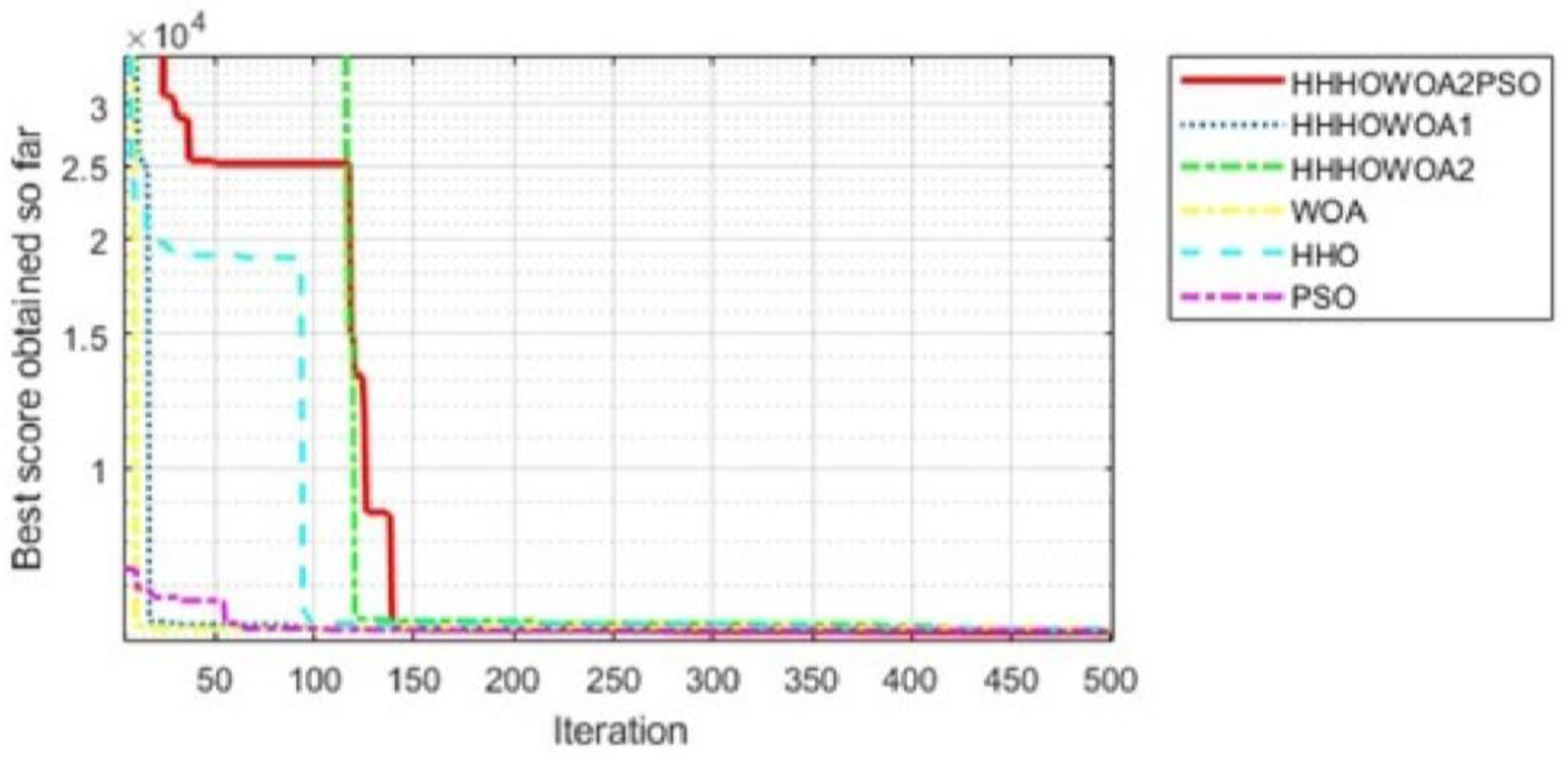
4.2. Comparison of Proposed Algorithms Among Themselves

In this section, the results attained with 30 runs of the F1–F23 functions using the proposed HHHOWOA1, HHHOWOA2, HHHOWOA1PSO (w = 0.1, Wc = 0.8), HHHOWOA1PSO (w = 0.3, Wc = 0.8), HHHOWOA2PSO (w = 0.1, Wc = 0.87), and HHHOWOA2PSO (w = 0.1, Wc = 0.99) algorithms are given in Table 4. In addition, internal comparisons among themselves and interpretation of the results are performed for the benchmark functions.
In the comparison among themselves, method HHHOWOA2PSO (w = 0.1, Wc = 0.99) achieved either better or equivalent average optimization values in 15 out of 23 functions, method HHHOWOA2PSO (w = 0.1, Wc = 0.87) in 14 out of 23 functions, method HHHOWOA1 in 10 out of 23 functions, method HHHOWOA2 in 8 out of 23 functions, method HHHOWOA1PSO (w = 0.3, Wc = 0.8) in 8 out of 23 functions, and method HHHOWOA1PSO (w = 0.1, Wc = 0.8) in 6 out of 23 functions. In general, it seems that all algorithms for F1–F4 are very close to 0, and there is only an exponential difference between them. This shows that, according to these functions, all the proposed algorithms successfully find the global optimum. However, HHHOWOA2PSO (w = 0.1, Wc = 0.87) provided the best results for functions F1 to F4 compared to the others.
For all algorithms, both F8 and F10 achieved consistently good and equivalent optimization values. Additionally, all the suggested algorithms for F9 and F11 successfully obtain the desired result of zero. Compared to the other proposed algorithms, method HHHOWOA1PSO (w = 0.1, Wc = 0.8) achieved the best optimization value for F12, and method HHHOWOA1PSO (w = 0.3, Wc = 0.8) reached the best optimization value for F13. F8-F13 functions can measure the ability of algorithms to escape the local optimum. Especially, the HHHOWOA1PSO algorithm can successfully escape from the local optimum according to the results. All the proposed algorithms obtain the best results for F14 and F18. For F19, method HHHOWOA2PSO (w = 0.1, Wc = 0.99) provided the result closest to the goal value. For F15-F17 and F20-F23, methods HHHOWOA1 and HHHOWOA2PSO (w = 0.1, Wc = 0.99) provided results closer to the goal value. As F14–F23 multimodal functions can measure the combination of the exploration and exploitation capabilities of an algorithm, this shows that the combination of these two phases in HHHOWOA1 and HHHOWOA2PSO (w = 0.1, Wc = 0.99) is balanced.

4.3. Comparison of the Proposed Approaches with the Literature

The results of the literature articles are compared with the proposed HHHOWOA1 and HHHOWOA2PSO (w = 0.1, Wc = 0.99) results in this section. To make a precise comparison with the literature, articles that used the same criteria are found as much as possible. Therefore, the literature algorithms with population, maximum iteration, and independent run numbers of 30, 500, and 30, respectively, were chosen. These are the HHO, GWO, PSO, WOA, and WOALFVWPSO algorithms [5,17,25,28].
Table 5 presents a comparison of the HHHOWOA1 and HHHOWOA2PSO results with the literature algorithms for the F1–F23 functions. According to the literature, the HHHOWOA1 and HHHOWOA2PSO approaches achieve the most optimal result, either better or with the same average fitness values, in 15 of the 23 functions and in 18 of the 23 functions, respectively. The proposed HHHOWOA1 algorithms achieved optimal results except for F1–F5, F12, F17, and F19. The proposedHHHOWOA2PSO algorithms achieved optimal results except for F2–F4, F17, and F19.
The HHO algorithm for F17 and F19 and the WOALFVWPSO algorithm for F2–F4 are better than the HHHOWOA2PSO algorithm. But the results of the HHO algorithm for F17 and F19 have been rounded. For the F1–F23 functions, Friedman rank tests have been performed on the average optimization results of all algorithms, and the average values of Friedman rank tests have been calculated. According to Friedman mean rank tests, it is seen that the HHHOWOA2PSO (w = 0.1, Wc = 0.99) algorithm has the best value in ranking for the F1–F23 functions.
Then, the following algorithms come in order: HHHOWOA1, HHO, WOALFVWPSO, GWO, the WOA, and PSO. When the proposed HHHOWOA2PSO and HHHOWOA1 algorithms are compared with the HHO algorithm over the F1–F7 benchmark functions, it is observed that the HHHOWOA2PSO algorithm outperforms the HHO algorithm in all seven functions, while the HHHOWOA1 algorithm outperforms the HHO algorithm in six out of these seven functions. Therefore, the strength and proficiency of these two proposed algorithms in the exploitation phase are better than those of the HHO algorithm. When the proposed HHHOWOA2PSO and HHHOWOA1 algorithms are compared with the HHO algorithm over the F8-F13 benchmark functions, they achieve the most optimal results, either better or with the same average fitness values, in six out of six functions and in five out of six functions, respectively. Therefore, the exploration stage and the ability of these two proposed algorithms to avoid getting stuck in local optima are better than those of the HHO algorithm. When the proposed HHHOWOA2PSO and HHHOWOA1 algorithms are compared with the HHO algorithm over the F14–F23 benchmark functions, they achieve the most optimal results, either better or with the same average fitness values, in 8 out of 10 functions and in 8 out of 10 functions, respectively. Therefore, the equilibrium between the exploitation and exploration stages of the optimization of these two proposed algorithms is better than that of the HHO algorithm.
In terms of the convergence curves, a comparison of the proposed HHHOWOA1 and HHHOWOA2PSO algorithms with the literature algorithms for some benchmark problems is shown in Figure 5. Especially, from the convergence curve graphs of F1 and F4, it can be observed that the proposed HHHOWOA1 and HHHOWOA2PSO algorithms converge better than the HHO algorithm and other algorithms at the point where it stagnates. When comparing the convergence curves of the two proposed methods, it can be seen that adding PSO allows the HHHOWOA2PSO algorithm to converge more effectively without stagnation, thus outperforming HHHOWOA1.

4.4. Statistical Analysis

The Friedman test is a non-parametric statistical technique used to compare ordinal data from multiple dependent groups. Its main purpose is to assess whether there are significant differences between the groups. A p-value below 0.05 suggests a significant difference between the groups.
In this study, since the functions used to test the algorithms have different target values, the results of the functions have been subtracted from the target values, and the absolute value has been taken. The obtained absolute difference values have been used in the Friedman’s mean rank test. For each function, the algorithm with the lowest value receives the first rank, and the other algorithms are assigned the subsequent ranks accordingly. Next, the average ranks for each algorithm are computed, and the algorithm with the lowest average rank is deemed the best performer across the 23 benchmark functions.
After calculating the absolute errors of the results of the proposed algorithms presented in Table 4 relative to the target value, the Friedman test was applied, and the p-value was found to be 9.9686 × 10⁻⁴. Therefore, it was understood that a significant difference existed between the groups. The Friedman mean results were found to be 3.6739 for HHHOWOA1, 3.7391 for HHHOWOA2, 4.1957 for HHHOWOA1PSO (w = 0.1, Wc = 0.8), 4.0435 for HHHOWOA1PSO (w = 0.3, Wc = 0.8), 2.8043 for HHHOWOA2PSO (w = 0.1, Wc = 0.87), and 2.5435 for HHHOWOA2PSO (w = 0.1, Wc = 0.99), respectively, as shown in Figure 6. According to the Friedman average ranking, the proposed HHHOWOA2PSO (w = 0.1, Wc = 0.99) algorithm demonstrates the best performance, the proposed HHHOWOA2PSO (w = 0.1, Wc = 0.87) algorithm demonstrates the second-best performance, and the HHHOWOA1 algorithm demonstrates the third-best performance across 23 benchmark functions.
After calculating the absolute errors of the results of the best two proposed algorithms and the other literature algorithms presented in Table 5 relative to the target value, the Friedman test was applied, and the p-value was found to be 5.9890 × 10⁻¹⁶. Therefore, it was understood that a significant difference existed between the groups. The Friedman average results were found to be 5.1087 for GWO, 3.6087 for WOALFVWPSO, 6.0000 for PSO, 5.6304 for the WOA, 3.2391 for HHO, 2.5217 for HHHOWOA1, and 1.8913 for HHHOWOA2PSO (w = 0.1, Wc = 0.99), respectively, as shown in Figure 7. According to the Friedman average ranking, the proposed HHHOWOA2PSO (w = 0.1, Wc = 0.99) algorithm demonstrates the best performance, the proposed HHHOWOA1 algorithm demonstrates the second-best performance, and the HHO algorithm demonstrates the third-best performance across 23 benchmark functions.

4.5. Application of the Proposed Approaches to Engineering Problems

The proposed HHHOWOA1, HHHOWOA2, and HHHOWOA2PSO algorithms are applied to engineering challenges, and their results are compared with those reported in prior publications. The maximum iterations, population size, and number of independent runs for these applications are set to 500, 30, and 30, respectively.

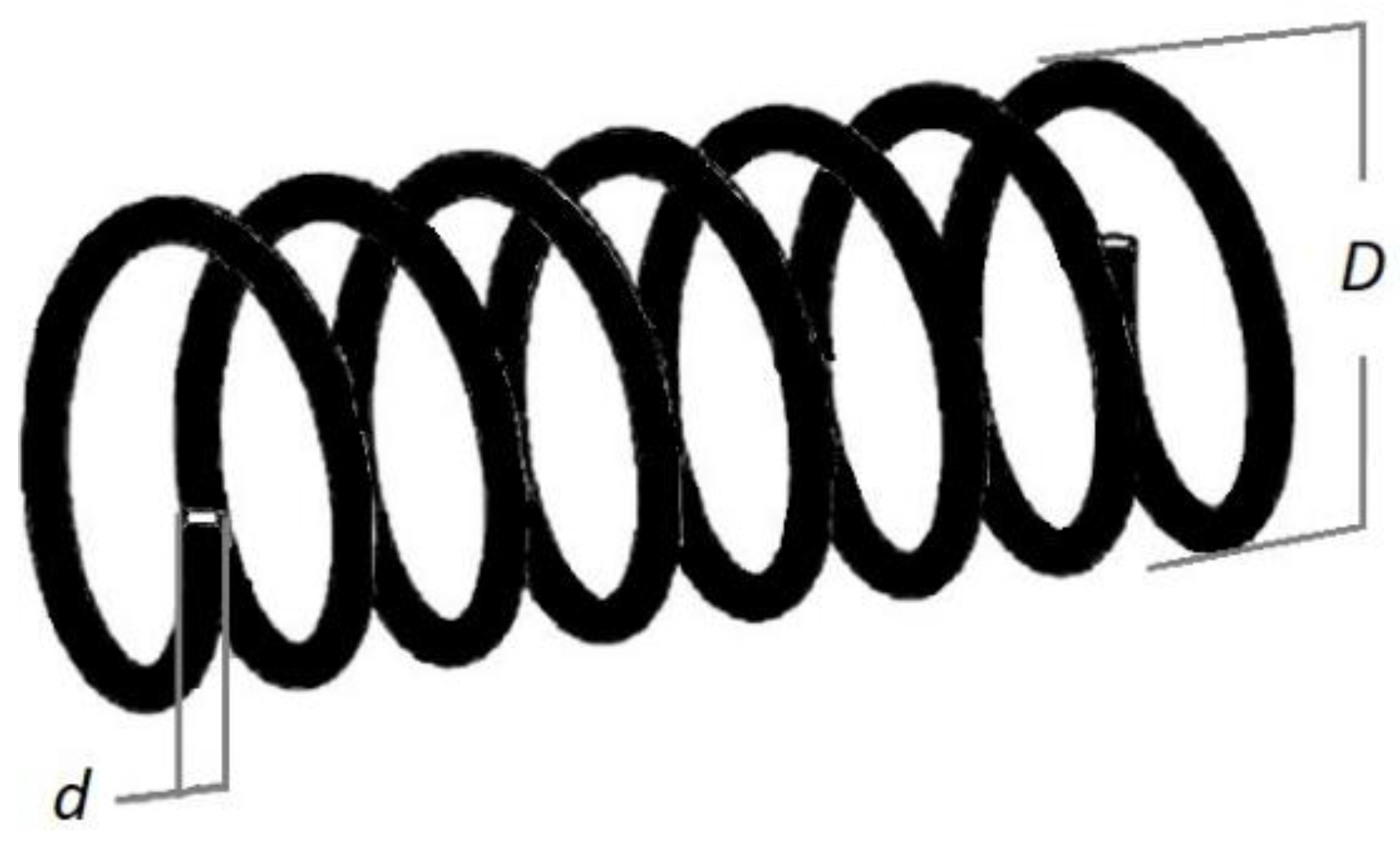
4.6. Tension–Compression Spring Design Problem

The purpose of this issue is to calculate the minimum weight of a tension–compression spring based on four limitations. These restrictions are limits on outside diameters (g4), surge frequency (g3), shear stress (g2), and minimum deflection (g1) [49]. This issue has three parameters: active coil number (N), average coil diameter (D), and wire diameter (d) [43]. This issue is addressed in Equations (31)–(36) [49]. This problem is shown in Figure 8.
Consider the following:
z = z 1   z 2   z 3 = d   D   N ,
Minimize the following:
f ( z ) = ( z 3 + 2 ) z 2 z 1 2
Subject to the following:
g 1 ( z ) = 1 z 2 3 z 3 71 , 785 z 1 4 0 ,
g 2 ( z ) = 4 z 2 2 z 1 z 2 12 , 566 ( z 2 z 1 3 z 1 4 ) + 1 5108 z 1 2 1 0 ,
g 3 ( z ) = 1 140.45 z 1 z 2 2 z 3 0 ,
g 4 ( z ) = z 1 + z 2 1.5 1 0 ,
Variable range as follows:
0.05 z 1 2 , 0.25 z 2 1.3 , 2 z 3 15 .
The best optimization and its variable values are found for this design problem. These values are compared to the literature, as given in Table 6. The HHHOWOA2, HHHOWOA1, and HHHOWOA2PSO algorithms are the most cost-effective, respectively. Then, the following algorithms come in order: HHO, GWO, RSRFT, MFO, the WOA, the SSA, the RFO, and the EDBO. Furthermore, Figure 9 illustrates the best optimization convergence curves for the proposed methods and the optimization algorithms they are based on, including the WOA, HHO, and PSO, in the context of the tension–compression spring design.

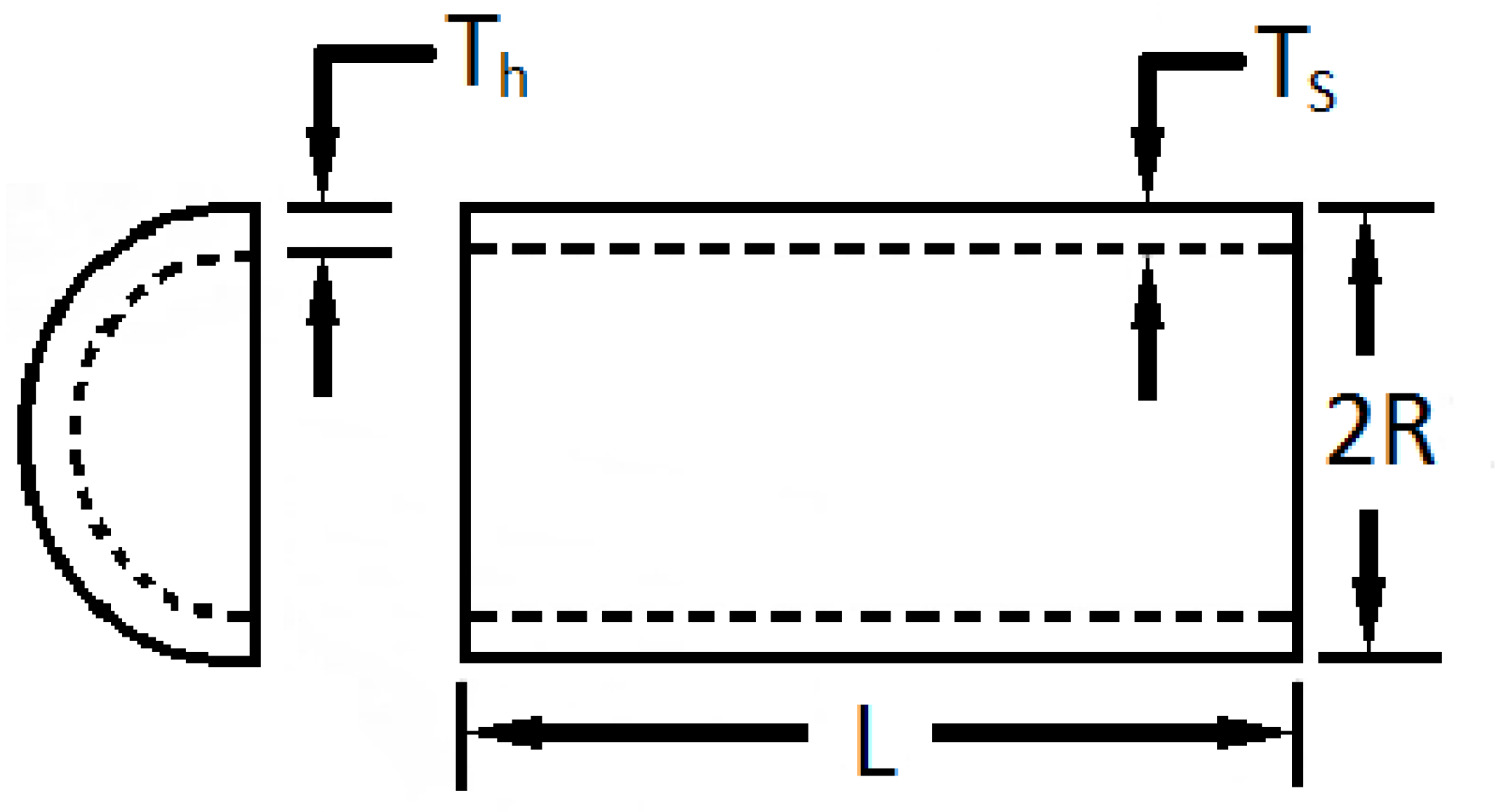
4.7. Pressure Vessel Design Problem

The purpose of this design is to minimize fabrication costs. The vessel has caps at both ends, and its head is hemispherical in shape. This design has four parameters. L, R, Th, and Ts represent the cylindrical length section without the head, inner radius, head thickness, and shell thickness, respectively. Also, this problem has four limitations, which are presented in Equations (37)–(42). The pressure vessel and the design parameters are shown in Figure 10 [28,50].
Consider the following:
z = z 1   z 2   z 3   z 4 = T s   T h   R   L ,
Minimize the following:
f ( z ) = 0.6224 z 1   z 3   z 4 + 1.7781 z 2   z 3 2 + 3.1661 z 1 2 z 4 + 19.84 z 1 2 z 3 ,
Variable range as follows:
0 z 1 99 ,   0 z 2 99 ,   10 z 3 200 ,   10 z 4 200 ,
Subjected to the following:
g 1 ( z ) = z 1 + 0.0193 z 3 0 ,
g 2 ( z ) = z 2 + 0.00954 z 3 0 ,
g 3 ( z ) = π z 3 2 z 4 4 3 π z 3 3 + 1 , 296 , 000 0 ,
g 4 ( z ) = z 4 240 0 ,
To compare with the literature, the variables of this problem were analyzed in two ways. First, the variables were examined as continuous. Second, the first two variables (Ts, Th) were analyzed as multiples of 0.0625 (material thickness), while the others were examined as continuous variables. Then, the best optimization and its variable values are found. These values are compared to the literature, as given in Table 7. In terms of the best optimization value, the recommended algorithms, HHHOWOA2PSO and HHHOWOA2, ranked first and second, respectively, for variables considered as continuous. Then, the following algorithms come in order: RSRFT, WOALFVWPSO, the EDBO, CIHHO, HHO, HHHOWOA1, MFO, the WOA, CPSO, and the RFO. Furthermore, Figure 11 illustrates the best optimization convergence curves for the proposed methods and the optimization algorithms they are based on, including the WOA, HHO, and PSO, in the context of the pressure vessel design.

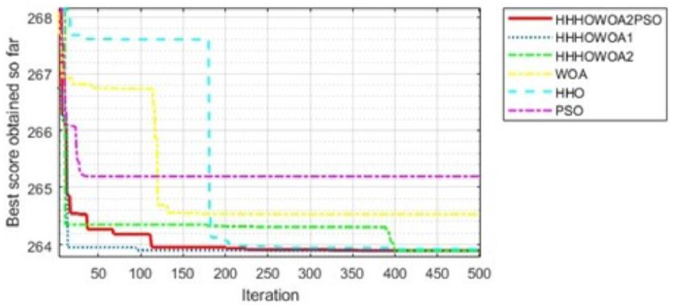
4.8. Three-Bar Truss Design Problem

The civil engineering optimization problem wants to find the minimal weight based on stress, deflection, and buckling limitations. This is accomplished by using two parameters. The different components of this problem are given in Figure 12. There are 4 nodes, numbered from 1 to 4, and 3 bars in the three-bar truss design, as shown in Figure 12. These nodes represent the connection points where the bars meet, forming the structure of the truss. Equations (43)–(47) express this problem [43].
Consider the following:
z = z 1   z 2 = A 1   A 2 ,
Minimize the following:
f ( z ) = ( 2 2 z 1 + z 2 ) l ,
Subject to the following:
g 1 ( z ) = 2 z 1 + z 2 2 z 1 2 + 2 z 1 z 2 P σ 0 ,
g 2 ( z ) = z 2 2 z 1 2 + 2 z 1 z 2 P σ 0 ,
g 3 ( z ) = 1 2 z 2 + z 1 P σ 0 ,
Variable range as follows:
0 z 1 ,   z 2 l ,  
where
l = 100   cm , P = 2   KN / cm 2 , σ = 2   KN / cm 2
The best optimization and its variable values are found for this problem. These values are compared to the literature, as shown in Table 8. RSRFT, CIHHO, PSO-DE, HHHOWOA1, HHHOWOA2, and HHO are the most cost-effective. Then, the following algorithms come in order: HHHOWOA2PSO, MFO, MBA, the EDBO, CS, and the RFO. Furthermore, Figure 13 illustrates the best optimization convergence curves for the proposed methods and the optimization algorithms they are based on, including the WOA, HHO, and PSO, in the context of the three-bar truss design.

5. Conclusions

This article proposes four innovative hybrid approaches based on HHO and the WOA, named HHHOWOA. These innovative hybrid approaches have significantly enhanced the performance of the HHO, WOA, and PSO algorithms, leading to improved outcomes. The search capacity for optimization has been enhanced, and the likelihood of the ideal value falling to a local minimum has been minimized.
The suggested approaches are evaluated on 23 benchmark functions and compared to published results using the same conditions. Among the four approaches, HHHOWOA1 and HHHOWOA2PSO have demonstrated more favorable results. According to the literature, the HHHOWOA1 and HHHOWOA2PSO approaches achieve the most optimal result, either better or with the same average fitness values, in 15 of the 23 functions and in 18 of the 23 functions, respectively. Friedman rank tests were run on the average optimization outcomes of all methods for these 23 functions, and the average values of Friedman rank tests were determined. According to the test findings, the two proposed algorithms are at the top of the success ranking for the F1–F23 function.
Furthermore, the proposed HHHOWOA1, HHHOWOA2, and HHHOWOA2PSO approaches are applied to three engineering benchmark issues, and the optimum values obtained are compared with the literature. In comparison to the literature algorithms, the offered algorithms are generally determined to be the most cost-effective. In addition, the computational complexity analysis of the proposed approaches was also performed.
In future research, the application of the proposed algorithms to data mining methods such as data clustering and feature selection can be realized. In addition, the proposed methods can be adapted and tested for solving optimization problems with multiple constraints and multiple objectives in future work.

Funding

The author declares that there is no funding for this work.

Institutional Review Board Statement

Not applicable.

Informed Consent Statement

Not applicable.

Data Availability Statement

Data are contained within this article.

Acknowledgments

The author is grateful to the Selcuk University Scientific Research Projects’ Coordinatorship for supporting this manuscript.

Conflicts of Interest

The author declares no conflicts of interest.

References

  1. Asghari, K.; Masdari, M.; Gharehchopogh, F.S.; Saneifard, R. Multi-swarm and chaotic whale-particle swarm optimization algorithm with a selection method based on roulette wheel. Expert Syst. 2021, 38, 44. [Google Scholar] [CrossRef]
  2. Wang, L.P.; Han, J.H.; Ma, F.J.; Li, X.K.; Wang, D. Accuracy design optimization of a CNC grinding machine towards low-carbon manufacturing. J. Clean. Prod. 2023, 406, 14. [Google Scholar] [CrossRef]
  3. Michalewicz, Z.; Fogel, D.B. How to Solve It: Modern Heuristics; Springer: New York, NY, USA, 2004. [Google Scholar]
  4. Hromkovič, J. Algorithmics for Hard Problems: Introduction to Combinatorial Optimization, Randomization, Approximation, and Heuristics; Springer: Berlin/Heidelberg, Germany, 2004. [Google Scholar]
  5. Uzer, M.S.; Inan, O. Application of improved hybrid whale optimization algorithm to optimization problems. Neural Comput. Appl. 2023, 35, 12433–12451. [Google Scholar] [CrossRef]
  6. Wang, G.; Guo, L. A Novel Hybrid Bat Algorithm with Harmony Search for Global Numerical Optimization. J. Appl. Math. 2013, 2013, 696491. [Google Scholar] [CrossRef]
  7. Irmak, B.; Karakoyun, M.; Gülcü, S. An improved butterfly optimization algorithm for training the feed-forward artificial neural networks. Soft Comput. 2023, 27, 3887–3905. [Google Scholar] [CrossRef]
  8. Nguyen, P.T. Construction site layout planning and safety management using fuzzy-based bee colony optimization model. Neural Comput. Appl. 2021, 33, 5821–5842. [Google Scholar] [CrossRef]
  9. Cheng, M.-Y.; Prayogo, D. Fuzzy adaptive teaching–learning-based optimization for global numerical optimization. Neural Comput. Appl. 2018, 29, 309–327. [Google Scholar] [CrossRef]
  10. Houssein, E.H.; Hosney, M.E.; Mohamed, W.M.; Ali, A.A.; Younis, E.M.G. Fuzzy-based hunger games search algorithm for global optimization and feature selection using medical data. Neural Comput. Appl. 2023, 35, 5251–5275. [Google Scholar] [CrossRef] [PubMed]
  11. Uzer, M.S.; Inan, O. A novel feature selection using binary hybrid improved whale optimization algorithm. J. Supercomput. 2023, 79, 10020–10045. [Google Scholar] [CrossRef]
  12. Hussain, K.; Mohd Salleh, M.N.; Cheng, S.; Shi, Y. Metaheuristic research: A comprehensive survey. Artif. Intell. Rev. 2019, 52, 2191–2233. [Google Scholar] [CrossRef]
  13. Meraihi, Y.; Gabis, A.B.; Mirjalili, S.; Ramdane-Cherif, A. Grasshopper Optimization Algorithm: Theory, Variants, and Applications. IEEE Access 2021, 9, 50001–50024. [Google Scholar] [CrossRef]
  14. Lourenço, H.R.; Martin, O.C.; Stützle, T. Iterated Local Search. In Handbook of Metaheuristics; Glover, F., Kochenberger, G.A., Eds.; Springer: Boston, MA, USA, 2003; pp. 320–353. [Google Scholar] [CrossRef]
  15. Kirkpatrick, S.; Gelatt, C.D.; Vecchi, M.P. Optimization by Simulated Annealing. Science 1983, 220, 671–680. [Google Scholar] [CrossRef]
  16. Voudouris, C.; Tsang, E. Guided local search and its application to the traveling salesman problem. Eur. J. Oper. Res. 1999, 113, 469–499. [Google Scholar] [CrossRef]
  17. Heidari, A.A.; Mirjalili, S.; Faris, H.; Aljarah, I.; Mafarja, M.; Chen, H.L. Harris hawks optimization: Algorithm and applications. Futur. Gener. Comput. Syst. 2019, 97, 849–872. [Google Scholar] [CrossRef]
  18. Kaya, E.; Gorkemli, B.; Akay, B.; Karaboga, D. A review on the studies employing artificial bee colony algorithm to solve combinatorial optimization problems. Eng. Appl. Artif. Intell. 2022, 115, 105311. [Google Scholar] [CrossRef]
  19. Kaur, S.; Awasthi, L.K.; Sangal, A.L.; Dhiman, G. Tunicate Swarm Algorithm: A new bio-inspired based metaheuristic paradigm for global optimization. Eng. Appl. Artif. Intell. 2020, 90, 103541. [Google Scholar] [CrossRef]
  20. Karaboga, D.; Basturk, B. A powerful and efficient algorithm for numerical function optimization: Artificial bee colony (ABC) algorithm. J. Glob. Optim. 2007, 39, 459–471. [Google Scholar] [CrossRef]
  21. Arora, S.; Anand, P. Binary butterfly optimization approaches for feature selection. Expert Syst. Appl. 2019, 116, 147–160. [Google Scholar] [CrossRef]
  22. Dhiman, G.; Kumar, V. Emperor penguin optimizer: A bio-inspired algorithm for engineering problems. Knowl.-Based Syst. 2018, 159, 20–50. [Google Scholar] [CrossRef]
  23. Kennedy, J.; Eberhart, R. Particle swarm optimization. In Proceedings of the ICNN’95-International Conference on Neural Networks, Perth, WA, Australia, 27 November–1 December 1995; pp. 1942–1948. [Google Scholar]
  24. Zhu, G.Y.; Zhang, W.B. Optimal foraging algorithm for global optimization. Appl. Soft Comput. 2017, 51, 294–313. [Google Scholar] [CrossRef]
  25. Mirjalili, S.; Mirjalili, S.M.; Lewis, A. Grey Wolf Optimizer. Adv. Eng. Softw. 2014, 69, 46–61. [Google Scholar] [CrossRef]
  26. Saremi, S.; Mirjalili, S.; Lewis, A. Grasshopper Optimisation Algorithm: Theory and application. Adv. Eng. Softw. 2017, 105, 30–47. [Google Scholar] [CrossRef]
  27. Mirjalili, S.; Gandomi, A.H.; Mirjalili, S.Z.; Saremi, S.; Faris, H.; Mirjalili, S.M. Salp Swarm Algorithm: A bio-inspired optimizer for engineering design problems. Adv. Eng. Softw. 2017, 114, 163–191. [Google Scholar] [CrossRef]
  28. Mirjalili, S.; Lewis, A. The Whale Optimization Algorithm. Adv. Eng. Softw. 2016, 95, 51–67. [Google Scholar] [CrossRef]
  29. Askarzadeh, A. A novel metaheuristic method for solving constrained engineering optimization problems: Crow search algorithm. Comput. Struct. 2016, 169, 1–12. [Google Scholar] [CrossRef]
  30. Furio, C.; Lamberti, L.; Pruncu, C.I. An Efficient and Fast Hybrid GWO-JAYA Algorithm for Design Optimization. Appl. Sci. 2024, 14, 9610. [Google Scholar] [CrossRef]
  31. Knypinski, L.; Devarapalli, R.; Gillon, F. The hybrid algorithms in constrained optimization of the permanent magnet motors. IET Sci. Meas. Technol. 2024, 18, 613–619. [Google Scholar] [CrossRef]
  32. Ramachandran, M.; Mirjalili, S.; Nazari-Heris, M.; Parvathysankar, D.S.; Sundaram, A.; Charles Gnanakkan, C.A.R. A hybrid Grasshopper Optimization Algorithm and Harris Hawks Optimizer for Combined Heat and Power Economic Dispatch problem. Eng. Appl. Artif. Intell. 2022, 111, 104753. [Google Scholar] [CrossRef]
  33. Naik, M.K.; Panda, R.; Wunnava, A.; Jena, B.; Abraham, A. A leader Harris hawks optimization for 2-D Masi entropy-based multilevel image thresholding. Multimed. Tools Appl. 2021, 80, 35543–35583. [Google Scholar] [CrossRef]
  34. Elaziz, M.A.; Heidari, A.A.; Fujita, H.; Moayedi, H. A competitive chain-based Harris Hawks Optimizer for global optimization and multi-level image thresholding problems. Appl. Soft Comput. 2020, 95, 106347. [Google Scholar] [CrossRef]
  35. Karaboga, D.; Basturk, B. On the performance of artificial bee colony (ABC) algorithm. Appl. Soft Comput. 2008, 8, 687–697. [Google Scholar] [CrossRef]
  36. Karaboga, D.; Gorkemli, B.; Ozturk, C.; Karaboga, N. A comprehensive survey: Artificial bee colony (ABC) algorithm and applications. Artif. Intell. Rev. 2014, 42, 21–57. [Google Scholar] [CrossRef]
  37. Loganathan, A.; Ahmad, N.S. A Hybrid HHO-AVOA for Path Planning of a Differential Wheeled Mobile Robot in Static and Dynamic Environments. IEEE Access 2024, 12, 25967–25979. [Google Scholar] [CrossRef]
  38. Prakasa, M.A.; Robandi, I.; Nishimura, R.; Djalal, M.R. A New Scheme of Harris Hawk Optimizer with Memory Saving Strategy (HHO-MSS) for Controlling Parameters of Power System Stabilizer and Virtual Inertia in Renewable Microgrid Power System. IEEE Access 2024, 12, 73849–73878. [Google Scholar] [CrossRef]
  39. Abd Elaziz, M.; Chelloug, S.; Alduailij, M.; Al-qaness, M.A.A. Boosted Reptile Search Algorithm for Engineering and Optimization Problems. Appl. Sci. 2023, 13, 3206. [Google Scholar] [CrossRef]
  40. Li, Q.H.; Shi, H.; Zhao, W.T.; Ma, C.L. Enhanced Dung Beetle Optimization Algorithm for Practical Engineering Optimization. Mathematics 2024, 12, 1084. [Google Scholar] [CrossRef]
  41. Ouyang, C.T.; Liao, C.; Zhu, D.L.; Zheng, Y.Y.; Zhou, C.J.; Zou, C.Y. Compound improved Harris hawks optimization for global and engineering optimization. Clust. Comput. 2024, 27, 9509–9568. [Google Scholar] [CrossRef]
  42. Shehadeh, H.A. A hybrid sperm swarm optimization and gravitational search algorithm (HSSOGSA) for global optimization. Neural Comput. Appl. 2021, 33, 11739–11752. [Google Scholar] [CrossRef]
  43. Mirjalili, S. Moth-flame optimization algorithm: A novel nature-inspired heuristic paradigm. Knowl.-Based Syst. 2015, 89, 228–249. [Google Scholar] [CrossRef]
  44. Xu, Y.B.; Zhang, J.Z. A Hybrid Nonlinear Whale Optimization Algorithm with Sine Cosine for Global Optimization. Biomimetics 2024, 9, 602. [Google Scholar] [CrossRef]
  45. Hubálovsky, S.; Hubálovská, M.; Matousová, I. A New Hybrid Particle Swarm Optimization-Teaching-Learning-Based Optimization for Solving Optimization Problems. Biomimetics 2024, 9, 8. [Google Scholar] [CrossRef]
  46. Mafarja, M.; Mirjalili, S. Whale optimization approaches for wrapper feature selection. Appl. Soft Comput. 2018, 62, 441–453. [Google Scholar] [CrossRef]
  47. Marini, F.; Walczak, B. Particle swarm optimization (PSO). A tutorial. Chemom. Intell. Lab. Syst. 2015, 149, 153–165. [Google Scholar] [CrossRef]
  48. Al-Tashi, Q.; Kadir, S.J.A.; Rais, H.M.; Mirjalili, S.; Alhussian, H. Binary Optimization Using Hybrid Grey Wolf Optimization for Feature Selection. IEEE Access 2019, 7, 39496–39508. [Google Scholar] [CrossRef]
  49. Heidari, A.A.; Ali Abbaspour, R.; Rezaee Jordehi, A. An efficient chaotic water cycle algorithm for optimization tasks. Neural Comput. Appl. 2017, 28, 57–85. [Google Scholar] [CrossRef]
  50. He, Q.; Wang, L. An effective co-evolutionary particle swarm optimization for constrained engineering design problems. Eng. Appl. Artif. Intell. 2007, 20, 89–99. [Google Scholar] [CrossRef]
  51. Liu, H.; Cai, Z.; Wang, Y. Hybridizing particle swarm optimization with differential evolution for constrained numerical and engineering optimization. Appl. Soft Comput. 2010, 10, 629–640. [Google Scholar] [CrossRef]
  52. Sadollah, A.; Bahreininejad, A.; Eskandar, H.; Hamdi, M. Mine blast algorithm: A new population based algorithm for solving constrained engineering optimization problems. Appl. Soft Comput. 2013, 13, 2592–2612. [Google Scholar] [CrossRef]
  53. Gandomi, A.H.; Yang, X.-S.; Alavi, A.H. Cuckoo search algorithm: A metaheuristic approach to solve structural optimization problems. Eng. Comput. 2013, 29, 17–35. [Google Scholar] [CrossRef]
Figure 1. HHO’s pseudocode.
Applsci 15 01355 g001
Figure 2. WOA’s pseudocode.
Applsci 15 01355 g002
Figure 3. HHHOWOA1 and HHHOWOA2 approaches’ pseudocode.
Applsci 15 01355 g003
Figure 4. HHHOWOA1PSO and HHHOWOA2PSO approaches’ pseudocode.
Applsci 15 01355 g004
Figure 5. Comparison of convergence curves of the proposed HHHOWOA1 and HHHOWOA2PSO algorithms with the literature algorithms on some benchmark problems.
Applsci 15 01355 g005aApplsci 15 01355 g005b
Figure 6. Mean ranks of proposed algorithms among themselves.
Applsci 15 01355 g006
Figure 7. Mean ranks of the proposed algorithms and the literature algorithms.
Applsci 15 01355 g007
Figure 8. Tension–compression spring design.
Applsci 15 01355 g008
Figure 9. The best optimization convergence curves of the proposed methods and other methods for the tension–compression spring design.
Applsci 15 01355 g009
Figure 10. Pressure vessel design.
Applsci 15 01355 g010
Figure 11. The best optimization convergence curves of the proposed methods and other methods for the pressure vessel design.
Applsci 15 01355 g011
Figure 12. Three-bar truss design.
Applsci 15 01355 g012
Figure 13. The best optimization convergence curves of the proposed methods and other methods for the three-bar truss design.
Applsci 15 01355 g013
Table 1. Unimodal functions (F1–F7).
Num. of
Func.
FunctionVar.
Num
Boundary (Lower–Upper)fmin
F 1 ( z ) i = 1 n z i 2 30LB = −100, UB = 1000
F 2 ( z ) i = 1 n z i + i = 1 n z i 30LB = −10, UB = 100
F 3 ( z ) i = 1 n ( j 1 i z j ) 2 30LB = −100, UB = 1000
F 4 ( z ) max i z i ,   1 i n 30LB = −100, UB = 1000
F 5 ( z ) i = 1 n 1 [ 100 ( z i + 1 z i 2 ) 2 + ( z i 1 ) 2 ] 30LB = −30, UB = 300
F 6 ( z ) i = 1 n ( [ z i + 0.5 ] ) 2 30LB = −100, UB = 1000
F 7 ( z ) i = 1 n i z i 4 + r a n d o m [ 0 , 1 ) 30LB = −1.28, UB = 1.280
Table 2. Multimodal functions (F8–F13).
Num. of
Func.
FunctionVar.
Num
Boundary (Lower–Upper)fmin
F 8 ( z ) i = 1 n z i sin ( z i ) 30LB = −500, UB = 500−418.9829×D
F 9 ( z ) i = 1 n z i 2 10 cos ( 2 π z i + 10 ) 30LB = −5.12, UB = 5.120
F 10 ( z ) 20 exp ( 0.2 1 n i = 1 n z i 2 ) exp ( 1 n i = 1 n cos ( 2 π z i ) ) + 20 + e 30LB = −32, UB = 320
F 11 ( z ) 1 4000 i = 1 n z i 2 i = 1 n cos ( z i i ) + 1 30LB = −600, UB = 6000
F 12 ( z ) π n 10 sin ( π y 1 ) + i = 1 n 1 ( y i 1 ) 2 1 + 10 sin 2 ( π y i + 1 ) + ( y n 1 ) 2
+ i = 1 n u ( z i , 10 , 100 , 4 )
y i = 1 + z i + 1 4 u ( z i , a , k , m ) = k ( z i a ) m 0 k ( z i a ) m z i > a a < z i < a z i < a
30LB = −50, UB = 500
F 13 ( z ) 0.1 sin 2 ( 3 π z 1 ) + i = 1 n ( z i 1 ) 2 1 + sin 2 ( 3 π z i + 1 )
+ ( z n 1 ) 2 1 + sin 2 ( 2 π z n ) + i = 1 n u ( z i , 5 , 100 , 4 )
30LB = −50, UB = 500
Table 3. Fixed-dimension multimodal functions (F14–F23).
Num. of
Func.
FunctionVar.
Num
Boundary (Lower–Upper)fmin
F 14 ( z ) ( 1 500 + j = 1 25 1 j + i = 1 2 ( z i a i j ) 6 ) 1 2LB = −65, UB = 651
F 15 ( z ) i = 1 11 a i z 1 ( b i 2 + b i z 2 ) b i 2 + b i z 3 + z 4 2 4LB = −5, UB = 50.00030
F 16 ( z ) 4 z 1 2 2.1 z 1 4 + 1 3 z 1 6 + z 1 z 2 4 z 2 2 + 4 z 2 4 2LB = −5, UB = 5−1.0316
F 17 ( z ) ( z 2 5.1 4 π 2 z 1 2 + 5 π z 1 6 ) 2 + 10 ( 1 1 8 π ) cos z 1 + 10 2LB = −5, UB = 50.398
F 18 ( z ) 1 + ( z 1 + z 2 + 1 ) 2 ( 19 14 z 1 + 3 z 1 2 14 z 2 + 6 z 1 z 2 + 3 z 2 2 ) ×
30 + ( 2 z 1 3 z 2 ) 2 × ( 18 32 z 1 + 12 z 1 2 + 48 z 2 36 z 1 z 2 + 27 z 2 2 )
2LB = −2, UB = 23
F 19 ( z ) i = 1 4 c i exp ( j = 1 3 a i j ( z j p i j ) 2 ) 3LB = 1, UB = 3−3.86
F 20 ( z ) i = 1 4 c i exp ( j = 1 6 a i j ( z j p i j ) 2 ) 6LB = 0, UB = 1−3.32
F 21 ( z ) i = 1 5 ( Z a i ) ( Z a i ) T + c i 1 4LB = 0, UB = 10−10.1532
F 22 ( z ) i = 1 7 ( Z a i ) ( Z a i ) T + c i 1 4LB = 0, UB = 10−10.4028
F 23 ( z ) i = 1 10 ( Z a i ) ( Z a i ) T + c i 1 4LB = 0, UB = 10−10.5363
Table 4. The comparison of the proposed algorithms for the F1–F23 functions.
Func
Num
fmin
(Target Value)
HHHOWOA1HHHOWOA2HHHOWOA1PSO
(w = 0.1, Wc = 0.8)
HHHOWOA1PSO
(w = 0.3, Wc = 0.8)
HHHOWOA2PSO
(w = 0.1, Wc = 0.87)
HHHOWOA2PSO
(w = 0.1, Wc = 0.99)
AveStdAveStdAveStdAveStdAveStdAveStd
F107.5688 × 10−1633.1435 × 10−1624.4183 × 10−27904.9168 × 10−22301.7489 × 10−18500000
F206.3749 × 10−1121.4659 × 10−1115.3520 × 10−1411.6592 × 10−1402.6277 × 10−1447.7444 × 10−1449.3859 × 10−1161.4463 × 10−1155.0998 × 10−16501.3642 × 10−1432.4035 × 10−143
F309.7687 × 10−862.6715 × 10−851.0246 × 10−24705.2309 × 10−1391.8573 × 10−1383.3371 × 10−1227.6236 × 10−1225.5734 × 10−29705.8706 × 10−2570
F407.2856 × 10−581.4966 × 10−573.3849 × 10−1407.6830 × 10−1405.9403 × 10−881.3481 × 10−875.7732 × 10−768.4847 × 10−765.1158 × 10−16305.1401 × 10−1438.5271 × 10−143
F501.58 × 10−21.28 × 10−21.80 × 10−21.5347 × 10−23.00 × 10−33.100 × 10−31.700 × 10−31.500 × 10−31.700 × 10−31.300 × 10−38.1582 × 10−35.99452 × 10⁻³
F605.5635 × 10−55.2482 × 10−56.9172 × 10−55.2127 × 10−56.4207 × 10−65.9199 × 10−66.4379 × 10−65.1401 × 10−65.6822 × 10−65.0890 × 10−64.7299 × 10−53.30251 × 10⁻⁵
F704.1742 × 10−51.2773 × 10−46.1309 × 10−51.3507 × 10−45.4657 × 10−56.6645 × 10−55.0220 × 10−59.1324 × 10−55.1236 × 10−51.3246 × 10−44.1047 × 10−51.2278 × 10⁻⁴
F8−418.9829 × D(30)−1.2569 × 1041.628 × 10−1−1.2569 × 1045.435 × 10−2−1.2569 × 1044.451 × 10−1−1.2569 × 1046.4170 × 10−1−1.2569 × 1048.7722 × 10−4−1.2569 × 1041.0250 × 10−1
F90000000000000
F1004.4409 × 10−1604.4409 × 10−1604.4409 × 10−1604.4409 × 10−1604.4409 × 10−1604.4409 × 10−160
F110000000000000
F1202.9442 × 10−63.3438 × 10−54.2180 × 10−63.0745 × 10−69.6399 × 10−76.0726 × 10−71.0427 × 10−66.6825 × 10−71.2621 × 10−68.3728 × 10−71.4922 × 10−61.3570 × 10⁻⁵
F1304.1390 × 10−54.4308 × 10−54.5853 × 10−53.2563 × 10−51.1479 × 10−58.4429 × 10−68.2899 × 10−65.8436 × 10−61.4609 × 10−51.2821 × 10−52.84662 × 10−52.10999 × 10⁻⁵
F1419.980 × 10−13.7366 × 10−109.980 × 10−13.1807 × 10−139.980 × 10−15.6249 × 10−99.980 × 10−16.5476 × 10−89.980 × 10−11.6636 × 10−79.980 × 10−13.16591 × 10−10
F150.000303.0959 × 10−42.8224 × 10−53.1268 × 10−44.0431 × 10−63.2521 × 10−48.9993 × 10−63.2340 × 10−41.0263 × 10−53.1874 × 10−43.2332 × 10−53.0873 × 10−42.5451 × 10⁻⁴
F16−1.0316−1.03164.3281 × 10−11−1.03164.8945 × 10−10−1.03141.3373 × 10−4−1.03141.5692 × 10−4−1.03161.8940 × 10−5−1.03168.81347 × 10−8
F170.3983.979 × 10−13.8425 × 10−60.39791.4877 × 10−80.39976.7899 × 10−23.979 × 10−19.3412 × 10−53.979 × 10−14.6079 × 10−53.979 × 10−11.8607 × 10−5
F1833.00002.9879 × 10−143.00001.1148 × 10−143.00032.9895 × 10−43.00032.4535 × 10−43.00003.2568 × 10−53.00008.0118 × 10−8
F19−3.86−3.86237.1386 × 10−4−3.86188.5670 × 10−4−3.85644.6 × 10−3−3.85597.3651 × 10−3−3.86179.5276 × 10−4−3.86159.7288 × 10−4
F20−3.32−3.31882.7279 × 10−3−3.31826.9643 × 10−2−3.27522.80 × 10−2−3.28512.20 × 10−2−3.30607.8 × 10−3−3.31912.1882 × 10−3
F21−10.1532−1.01531 × 1011.0309 × 10−4−1.01529 × 1012.3945 × 10−4−9.88681.767 × 10−1−1.00392 × 1016.43 × 10−2−1.00735 × 1013.66 × 10−2−1.01530 × 1011.5709 × 10−4
F22−10.4028−1.04027 × 1012.4422 × 10−4−1.04027 × 1011.6608 × 10−4−1.00626 × 1011.696 × 10−1−1.02935 × 1017.40 × 10−2−1.03223 × 1015.26 × 10−2−1.04028 × 1011.6801 × 10−4
F23−10.5363−1.05363 × 1011.4095 × 10−4−1.05362 × 1011.7339 × 10−4−1.02332 × 1011.818 × 10−1−1.03978 × 1018.14 × 10−2−1.04300 × 1015.85 × 10−2−1.05363 × 1011.0364 × 10−4
Friedman mean rank results3.6739 3.7391 4.1957 4.0435 2.8043 2.5435
Friedman rank3 4 6 5 2 1
Table 5. The comparison of the HHHOWOA1 and HHHOWOA2PSO results with the literature for the F1–F23 functions.
Func
Num
fmin
(Target Value)
GWO [25]WOALFVWPSO [5]PSO [28]WOA [28]HHO [17]HHHOWOA1HHHOWOA2PSO
(w = 0.1, Wc = 0.99)
AveStdAveStdAveStdAveStdAveStdAveStdAveStd
F106.5900 × 10−286.3400 × 10−5001.3600 × 10−42.0200 × 10−41.4100 × 10−304.9100 × 10−303.95 × 10−971.72 × 10−967.5688 × 10−1633.1435 × 10−16200
F207.1800 × 10−172.9014 × 10−26.1126 × 10−18604.2144 × 10−24.5421 × 10−21.0600 × 10−212.3900 × 10−211.56 × 10−516.98 × 10−516.3749 × 10−1121.4659 × 10−1111.3642 × 10−1432.4035 × 10−143
F303.2900 × 10−67.9150 × 1014.9407 × 10−32307.0126 × 1012.2119 × 1015.3900 × 10−72.9300 × 10−61.92 × 10−631.05 × 10−629.7687 × 10−862.6715 × 10−855.8706 × 10−2570
F405.6100 × 10−71.3151 × 1007.0830 × 10−17501.0865 × 1003.1704 × 10−17.2581 × 10−23.9747 × 10−11.02 × 10−475.01 × 10−477.2856 × 10−581.4966 × 10−575.1401 × 10−1438.5271 × 10−143
F502.6813 × 1016.9905 × 1012.7672 × 1014.3000 × 10−19.6718 × 1016.0116 × 1012.7866 × 1017.6363 × 10−11.32 × 10−21.87 × 10−21.58 × 10−21.28 × 10−28.1582 × 10−35.99452 × 10−3
F608.1658 × 10−11.2600 × 10−42.6074 × 10−12.2076 × 10−11.0200 × 10−48.2800 × 10−53.1163 × 1005.3243 × 10−11.15 × 10−41.56 × 10−45.5635 × 10−55.2482 × 10−54.7299 × 10−53.30251 × 10−5
F702.2130 × 10−31.0029 × 10−16.0582 × 10−55.8660 × 10−51.2285 × 10−14.4957 × 10−21.4250 × 10−31.1490 × 10−31.40 × 10−41.07 × 10−44.1742 × 10−51.2773 × 10−44.1047 × 10−51.2278 × 10⁻⁴
F8−418.9829 × D(30)−6.1231 × 10³−4.0874 × 10³−5.2568 × 1031.3258 × 103−4.8413 × 1031.1528 × 103−5.0808 × 1036.9580 × 102−1.25 × 1041.47 × 102−1.2569 × 1041.628 × 10−1−1.2569 × 1041.0250 × 10−1
F903.1052 × 10−14.7356 × 101004.6704 × 1011.1629 × 10100000000
F1001.0600 × 10−137.7835 × 10−28.8818 × 10−1602.7602 × 10−15.0901 × 10−17.4043 × 1009.8976 × 1008.88 × 10−164.01 × 10−314.4409 × 10−1604.4409 × 10−160
F1104.4850 × 10−36.6590 × 10−3009.2150 10−37.7240 × 10−32.8900 × 10−41.5860 × 10−3000000
F1205.3438 × 10−22.0734 × 10−22.3036 × 10−21.4120 × 10−26.9170 × 10−32.6301 × 10−23.3968 × 10−12.1486 × 10−12.08 × 10−61.19 × 10−52.9442 × 10−63.3438 × 10−51.4922 × 10−61.3570 × 10⁻⁵
F1306.5446 × 10−14.4740 × 10−34.5032 × 10−12.4475 × 10−16.6750 × 10−38.9070 × 10−31.8890 × 1002.6609 × 10−11.57 × 10−42.15 × 10−44.1390 × 10−54.4308 × 10−52.84662 × 10−52.10999 × 10−5
F1414.0425 × 1004.2528 × 1001.1968 × 1004.0440 × 10−13.6272 × 1002.5608 × 1002.1120 × 1002.4986 × 1009.98 × 10−19.23 × 10−19.980 × 10−13.7366 × 10−109.980 × 10−13.16591 × 10−10
F150.000303.3700 × 10−46.2500 × 10−43.2711 × 10−41.3308 × 10−55.7700 × 10−42.2200 × 10−45.7200 × 10−43.2400 × 10−43.10 × 10−41.97 × 10−43.0959 × 10−42.8224 × 10−53.0873 × 10−42.5451 × 10⁻⁴
F16−1.0316−1.0316 × 100−1.0316 × 100−1.0316 × 1003.7458 × 10−5−1.0316 × 1006.2500 × 10−16−1.0316 × 1004.2000 × 10−7−1.03 × 1006.78 × 10−16−1.03164.3281 × 10−11−1.03168.81347 × 10−8
F170.3983.9789 × 10−13.9789 × 10−13.9804 × 10−11.9193 × 10−43.9789 × 10−103.9791 × 10−12.7000 × 10−53.98 × 10−12.54 × 10−63.979 × 10−13.8425 × 10−63.979 × 10−11.8607 × 10−5
F1833.0000 × 1003.0000 × 1003.0000 × 1003.0908 × 10−73.0000 × 1001.3300 × 10−153.0000 × 1004.2200 × 10−153.00 × 10003.00002.9879 × 10−143.00008.0118 × 10−8
F19−3.86−3.8626 × 100−3.8628 × 100−3.8626 × 1008.9319 × 10−5−3.8628 × 1002.5800 × 10−15−3.8562 × 1002.7060 × 10−3−3.86 × 1002.44 × 10−3−3.86237.1386 × 10−4−3.86159.7288 × 10−4
F20−3.32−3.2865 × 100−3.2506 × 100−3.3022 × 1003.5700 × 10−2−3.2663 × 1006.0516 × 10−2−2.9811 × 1003.7665 × 10−1−3.322 × 1001.37406 10−1−3.31882.7279 × 10−3−3.31912.1882 × 10−3
F21−10.1532−1.0151 × 101−9.1402 × 100−9.8275 × 1009.2493 × 10−1−6.8651 × 1003.0196 × 100−7.0492 × 1003.6296 × 100−1.01451 × 1018.85673 × 10−1−1.01531 × 1011.0309 × 10−4−1.01530 × 1011.5709 × 10−4
F22−10.4028−1.0402 × 101−8.5844 × 100−1.0119 × 1019.5309 × 10−1−8.4565 × 1003.0871 × 100−8.1818 × 1003.8292 × 100−1.04015 × 1011.352375 × 100−1.04027 × 1012.4422 × 10−4−1.04028 × 1011.6801 × 10−4
F23−10.5363−1.0534 × 101−8.5590 × 100−1.0397 × 1011.0899 × 10−1−9.9529 × 1001.7828 × 100−9.3424 × 1002.4147 × 100−1.05364 × 1019.27655 × 10−1−1.05363 × 1011.4095 × 10−4−1.05363 × 1011.0364 × 10−4
Friedman mean rank results5.1087 3.6087 6.0000 5.6304 3.2391 2.5217 1.8913
Friedman rank5 4 7 6 3 2 1
Total number of the most optimum results obtained by comparing the proposed methods one by one according to the literature15 18
Table 6. Comparison of the results from the literature and the proposed HHHOWOA1, HHHOWOA2, and HHHOWOA2PSO algorithms for the tension–compression spring design.
AlgorithmsOptimum VariablesOptimum Cost
dDN
GWO [25]0.051690.35673711.288850.012666
MFO [43]0.0519944570.3641093210.8684218620.0126669
SSA [27]0.0512070.34521512.0040320.0126763
WOA [28]0.0512070.34521512.0040320.0126763
HHO [17]0.0517963930.35930535511.1388590.012665443
RSRFT [39]0.051471460.351505011.60131410.01266617
RFO [39]0.0526670110.380668010.02139250.0126934
EDBO [40]0.05001560.3177713.77780.012718751
HHHOWOA10.05177091620.358690153911.1742592080.0126653548
HHHOWOA20.05167259100.356321643711.3122254670.0126652377
HHHOWOA2PSO0.05169018570.356743140411.28765181730.0126654334
Table 7. Comparison of the results from the literature and the proposed HHHOWOA1, HHHOWOA2, and HHHOWOA2PSO algorithms for the pressure vessel design.
AlgorithmsOptimum VariablesOptimum Cost
TsThRL
WOALFVWPSO [5]0.78315960.394497940.354392005955.7996
CPSO [50]0.81250.437542.091266176.74656061.0777
MFO [43]0.81250.437542.098445176.6365966059.7143
WOA [28]0.81250.437542.0982699176.6389986059.741
HHO [17]0.817583830.407292742.09174576176.71963526000.46259
RSRFT [39]0.816122570.40340994942.2861349174.3250785953.4364
RFO [39]0.814250.4452142.20231176.621456113.3195
EDBO [40]0.78274960.394340.385942005957.489796
CIHHO [41]1.070550.5286355.3885460.6154685962.00814
HHHOWOA10.80496340.389070940.88383192.64676023.1709
0.81250.437542.0974671176.648721356059.8335
HHHOWOA20.78185550.392074540.319622005933.5439
0.81250.437542.095787915176.669531546060.0380
HHHOWOA2PSO0.78699230.388886740.77421193.78985901.0625
0.81250.437542.0984444394176.637682376059.7395
Table 8. Comparison of the results from the literature and the proposed HHHOWOA1, HHHOWOA2, and HHHOWOA2PSO for the three-bar truss design.
AlgorithmsOptimum VariablesOptimum Cost
A1A2
PSO-DE [51]0.78867510.4082482263.8958433
MFO [43]0.7882447709319220.409466905784741263.895979682
MBA [52]0.7882447710.409466905784741263.8959797
CS [53]0.788670.40902263.9716
HHO [17]0.7886628160.4082831338329263.8958434
RSRFT [39]0.788750520.4080351263.89584
RFO [39]0.753560.55373268.51195
EDBO [40]0.788210.40958263.8979156
CIHHO [41]0.788290.40934263.89584
HHHOWOA10.788673974360.4082515721132263.8958433
HHHOWOA20.78867181687990.4082576744595263.89584338
HHHOWOA2PSO0.7885479515396480.4086082820095263.89586973
Disclaimer/Publisher’s Note: The statements, opinions and data contained in all publications are solely those of the individual author(s) and contributor(s) and not of MDPI and/or the editor(s). MDPI and/or the editor(s) disclaim responsibility for any injury to people or property resulting from any ideas, methods, instructions or products referred to in the content.

